Using Fay–Herriot Models and Variable Radius Plot Data to Develop a Stand-Level Inventory and Update a Prior Inventory in the Western Cascades, OR, United States

Introduction

Stands are the primary unit for tactical–operational planning and management. A stand is an area or polygon with a relatively homogeneous forest structure and different from surrounding areas in terms of structure, composition, or management objectives. The size of a forest stand typically ranges from about 1 to 20–40 ha, and obtaining stand-level information is critical to inform management and planning decisions (Breidenbach et al., 2018; Mauro et al., 2019). Traditional forest inventories produce stand-level information using field surveys or stand exams where it is common to use variable radius plots (VRPs). These field surveys allow obtaining estimates for different variables of interest for the forest managers and assessing the quality of those surveys using methods described in the forest inventory literature.

Remote sensing inventories typically follow an area-based approach (ABA), where fixed area plots and remote sensing data are combined to produce maps with estimates of forest attributes at resolutions in the range of 10–30 m (Næsset, 2002). This methodology has been extensively used with lidar (e.g., Maltamo et al., 2004; González-Ferreiro et al., 2012; Babcock et al., 2015; Fekety et al., 2018), data from other sensors such as Landsat (LeMay et al., 2008; Pflugmacher et al., 2012) or Sentinel I and II (Forkuor et al., 2020), or different combinations of sensors (e.g., Vafaei et al., 2018; Forkuor et al., 2020). This methodology is well known and produces, in a very efficient manner, estimates in high-resolution grids (i.e., 10–30 m resolution) for a large number of forest attributes. These estimates can be summarized to generate stand-level maps for forest planning tasks. Besides, several studies have conducted small area estimation analysis showing that, with this methodology it is possible to obtain not only stand-level estimates of forest attributes but also measures of uncertainty for those stand-level estimates (Mauro et al., 2016, 2019; Breidenbach et al., 2018; Frank et al., 2020). Stand-level measures of uncertainty are a desirable output of any inventory method because they can be used as a measure of quality control. Reported uncertainties can be used to identify stands with more unreliable estimates that can be targeted in further field measurements efforts, saving resources for field data collections. Furthermore, even when additional ground measurements are not an option, stand-level measures of uncertainty are useful and can be incorporated in decision making processes and sensitivity analyses.

While the ABA method has been extensively developed during the last decade, it presents several drawbacks for operational inventories. This methodology’s main problem is that it is based on using fixed-radius plots with accurate coordinates. The collection of that kind of ground information is costly on a per plot basis or stand when stands are the sample units (Hummel et al., 2011). Fixed-radius plot inventories are efficient at the level of a whole landscape or project area (Hudak et al., 2014), which is typically stratified to distribute the sample plots across the range of stand structure conditions without regard to stand boundaries. However, for stand-level inventory, collecting fixed-radius plot data with highly accurate GPS coordinates requires more resources per sampled stand than typical stand exams based on VRP. This is because in the later, field plot coordinates are not recorded or are obtained using less expensive low-grade GPS equipment. Recent studies have demonstrated that it is possible to use VRP combined with remote sensing data in several ways. One possibility is to optimize the basal area factor (BAF) used in the VRP to the stand structure variation (Deo et al., 2016), or to use VRP and a constant BAF, using arbitrary but consistent support areas for the remote sensing predictors throughout the study area and operate as in the traditional ABA method (Grafström et al., 2017). While these methods are very interesting for operational inventories because they allow using VRP data, they do not eliminate the need to obtain accurate coordinates for the VRP. Another option that fits better with standard practices for stands exams is the use of Fay–Herriot (FH), models (Fay and Herriot, 1979). These models are sometimes referred to as stand-level models in forestry contexts and allow combining remote sensing data with different ground measurements in stands, eliminating the need for precise coordinates for ground measurements.

While traditional ABA models are developed considering field plots as the primary modeling unit, FH models operate at a coarser scale. FH models are developed with stands as the primary element. This implies several departures from traditional ABA models. One difference is that auxiliary information for FH models needs to be associated with stands for operational inventories (Goerndt et al., 2011; Mauro et al., 2017; Green et al., 2019) or with larger-scale domains such as counties for national inventories (Coulston et al., 2021). For example, stand-level summaries of lidar variables have been used in previous studies using FH models in stand-level forest inventories in Europe and the United States (Magnussen et al., 2017; Mauro et al., 2017; Ver Planck et al., 2018). But the most critical difference between FH and traditional ABA models is that ground information for the modeling units of FH models is typically incomplete. Fixed radius plots used in traditional ABA models are exhaustive and all or most of the trees within the plots are measured. This allows treating forest attributes (i.e., response variables) computed for the plots as known quantities. However, in operational settings stands are never fully measured; instead, they are sampled with many field plots that can vary between stands. This implies that the response variables used to develop stand-level FH models are subject to sampling errors that need to be accounted for in the modeling stage. FH models include a variance component to account for these sampling errors and can be seen as measurement error models where the response used for modeling has an inherent uncertainty because it comes from a sample and not from a complete measurement.

The coarse resolution of stand-level FH models can be a drawback for certain applications. However, FH models have advantages in terms of flexibility and data requirements over ABA methods. The most interesting properties of FH models are: (1) that they can be developed with any ground measurement from which it is possible to obtain unbiased estimators for stand-level attributes and their associated variances (i.e., VRP, transects, and sector plots) and (2) that they eliminate the need to record precise plot coordinates in the field (Goerndt et al., 2011; Ver Planck et al., 2018). Thus, FH models can use VRP data and plots without accurate GPS coordinates, making them a very appealing alternative for operational forest inventories based on lidar or other remote sensing auxiliary information sources. Despite their potential, very few applications of stand-level FH models exist in forest inventory literature and are focused on developing a new inventory using available auxiliary information. In this manuscript, we aim to analyze two possible scenarios where FH models can be used to combine remote sensing data and VRP data from stand exams. These scenarios or cases are:

1. Case 1: Developing a new stand-level inventory using recently collected lidar auxiliary information for an area where no fixed radius plot data is available.

2. Case 2: Updating an old remote-sensing-based inventory combining the same ground data used in Case 1 with remote sensing datasets developed at regional scales and with no access restrictions. The old remote sensing-based inventory was developed 5 years prior to the ground data collection. The auxiliary information included climate data, topographic variables, and spectral changes in Landsat images. These auxiliary variables aimed at capturing possible changes in the study area during the years between the old-remote sensing inventory and the updating date.

Both cases under analysis use stand exams based on VRP from the US Forest Service Field Sampled Vegetation (FSVeg) database but they can be directly replicated in many other areas managed by the US Forest Service or in other regions in the world.

Materials and Methods

Study Area

The study area comprises 31,209 ha inside the Willamette National Forest, OR, United States covered by different remote sensing datasets that include a recent lidar acquisition and a 30 m resolution map with above-ground biomass (AGB) predictions (Figure 1). Details on these datasets are provided in sections “Case 1: Fay–Herriot Models for New Inventories” and “Case 2: Fay–Herriot Models to Update Inventories.” Elevations range from 450 to 1700 m above sea level. Two forks of the Santiam river cross the study area from East to West and have numerous tributaries that form a complex drainage network where slopes do not have a dominant orientation. Conifers dominate vegetation with Douglas-fir, Pseudotsuga menziesii (Mirb) Franco, the most abundant species, and other conifers such as noble fir, Abies procera Rehder, silver fir, Abies amabilis Douglas ex J.Forbes, western hemlock, Tsuga heterophylla (Raf.) Sarg., and western red cedar, Thuja plicata Donn ex D.Don, as secondary species with a much lower abundance. Hardwood species have a minor presence with red alder, Alnus rubra Bong, and golden chinquapin, Chrysolepis chrysophylla (Douglas ex Hook.) Hjelmq., as the most important species in this group.

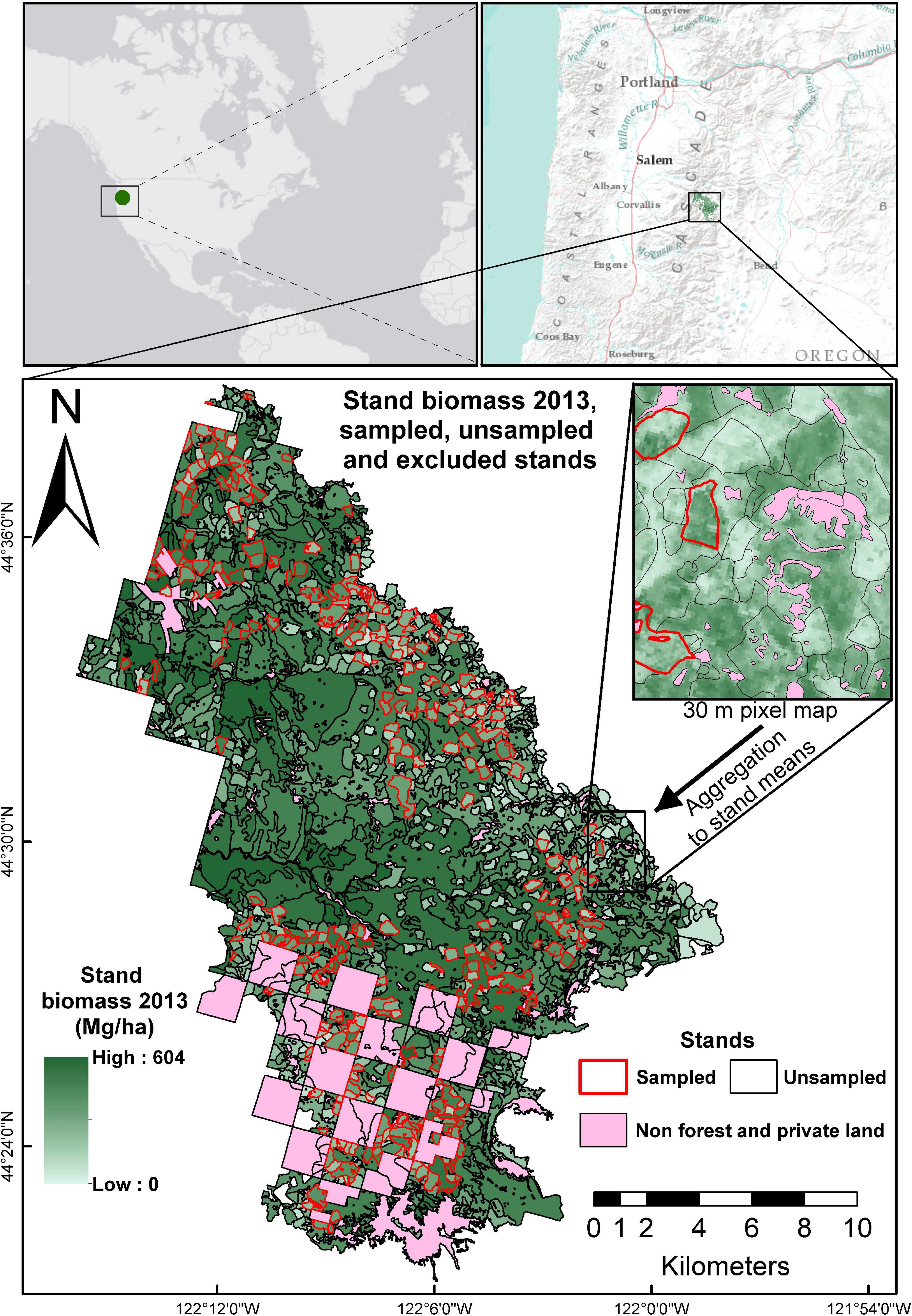
Figure 1. Location of the study area. In pink are stands excluded from the analysis because they were not covered by the remote sensing inventory from 2013. Stands in green color with red outline are sampled stands; and green stands with black outline are unsampled stands.

The study area contains 1616 stands with different management goals. Stand boundaries are the result of a continuous effort performed by forest managers in the study area and is based on the management history, structure, and composition of the forest. Stands are classified according to their management objectives into “Natural” and “Managed” (Figure 2). While the terms natural and managed can be the subject of lengthy discussions, we will keep this terminology as it is used in the FSVeg database. There are 696 natural stands and 920 managed stands. Natural stands occupy approximately two-thirds of the area. They are typically of larger size (i.e., average size = 31.04 ha, median size = 11.61 ha) than managed stands (i.e., average size = 9.90 ha, median size = 7.94 ha) (Figure 2). Managed stands have a past history of silviculture entry and often include artificial regeneration. In most cases, even-aged structures are subject to thinning and logging operations. Natural stands are subject to less intense management and tend to have larger dimensions and a larger internal variability in forest structure and ages (Figure 2).

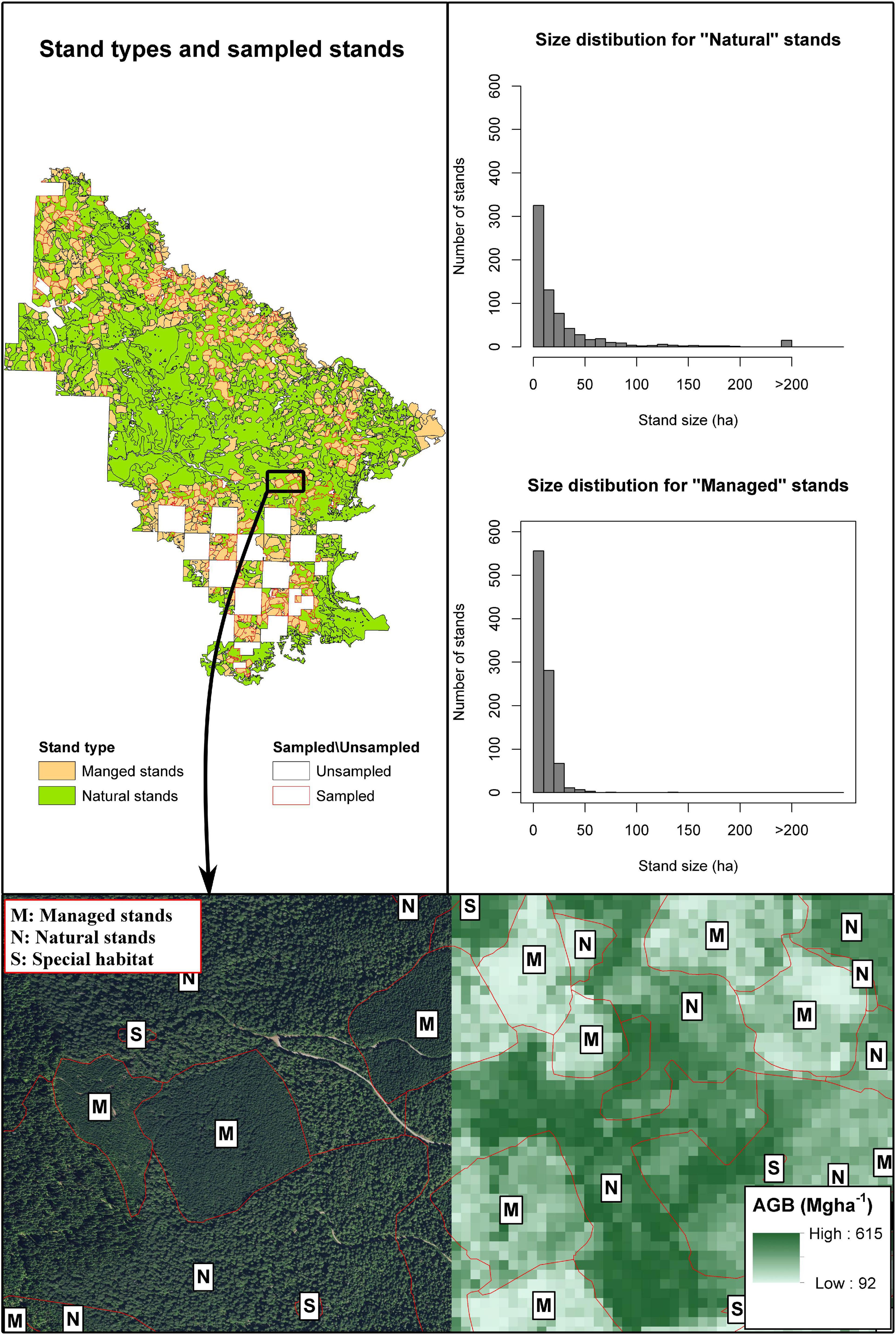
Figure 2. Upper left panel displays the location of natural and managed stands. Upper right and middle right panels display the size distribution within the study area for natural and managed stands, respectively. Bottom panel, sampled area showing the orthophoto on the western side and the CMS AGB map on the eastern side of the image. Managed stands are labeled with the letter M, natural stands are labeled with the letter N, and special habitat areas (small size non-forested polygons within stands) are labeled with letter S.

Sampled Stands and Field Sampled Vegetation Ground Data

In total, 37 natural and 238 managed stands in the study area were sampled in 2018 by field crews that used VRP with BAFs that changed depending on the stand characteristics. Natural and managed sampled stands were selected by forest managers in the region using a randomize procedure and also expert knowledge to ensure that most prevalent forest types were present in the sample. The proportion of natural stands sampled (i.e., 5.31%) was about five times smaller than the proportion of managed stands sampled (i.e., 25.86%). This reflects the larger information needs for the managed stands derived from their more intensive sylviculture. VRP were randomly located within the stands by the field crews. The number of VRP collected in the 37 sampled natural stands was 157 and the number of plots in the 238 sampled managed stands was 943 plots. The number of field plots in the sampled stands varied from 2 to 18, but 3, 4, and 5 were the most frequent number of field plots per stand (Figure 3). The field plot density, for the entire study area (i.e., including sampled and unsampled stands), was 0.017 plots ha^–1 for natural stands (1 plot every 58.01 ha) and 0.044 plots ha^–1 for managed stands (1 plot every 22.90 ha). For each VRP, the species, diameter at breast height (dbh), height (ht), and the live or dead status of each selected tree were recorded. Field crews used standard devices to measure dbh (i.e., caliper or logger’s tape) and ht (i.e., hypsometer or laser rangefinder). Finally, the BAF used in the plot allowed computing an expansion factor for each tree in the plot.

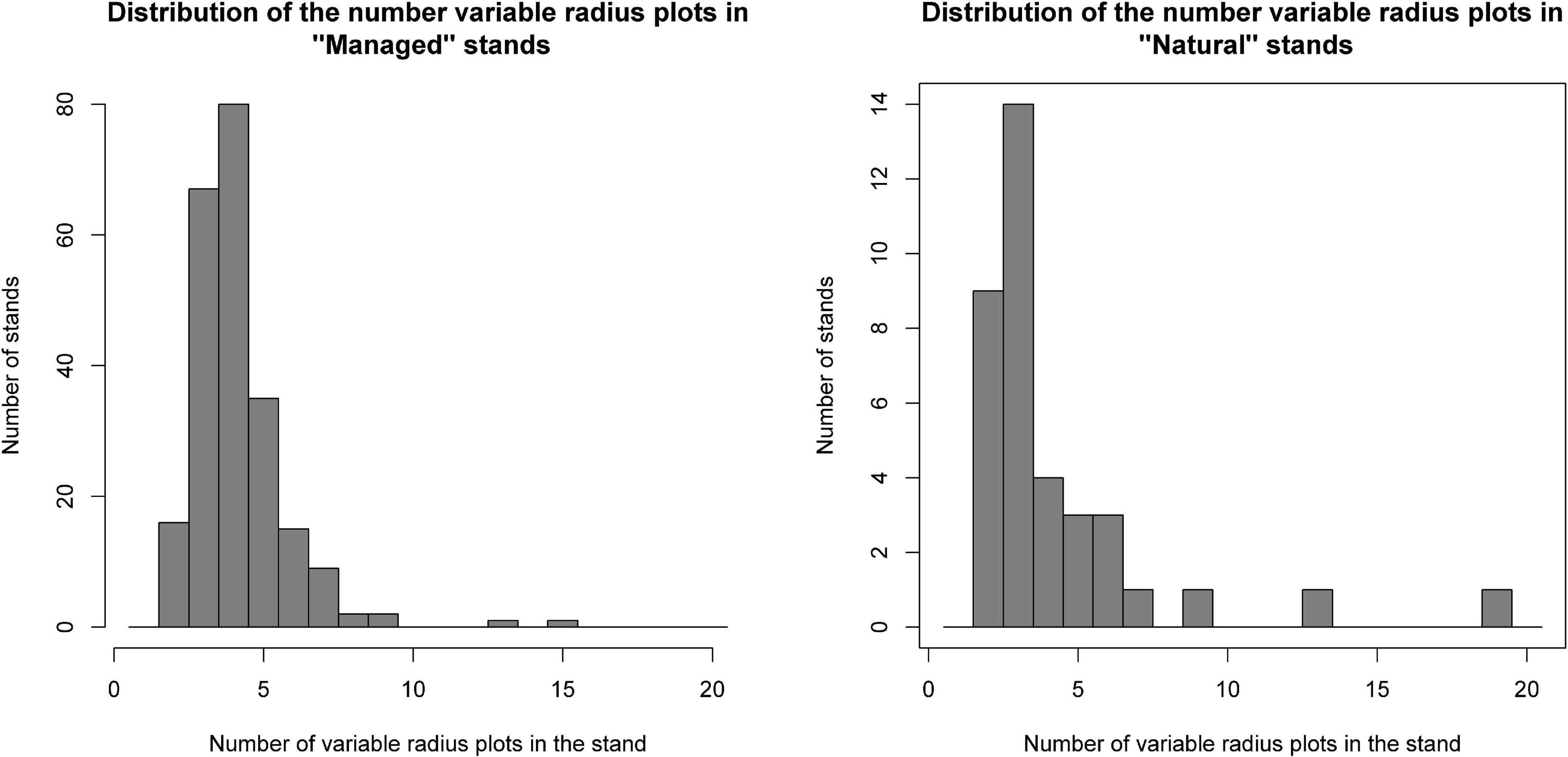
Figure 3. Distribution of the number of VRP per sampled stand in natural and managed stands.

Parameter of Interest

For both Case 1 and Case 2, we considered estimating, for every stand in the study area, the total of AGB, and merchantable volume (V), for the year 2018, both expressed on a per unit area basis. Thus, for every stand, the unknown parameter of interest was

when considering AGB and

when considering V. In equations 1, 2 AGB_ti and V_ti are the AGB and V of the t-th tree in the i-th stand, and N_i and A_i are, respectively, number of trees and the area of the i-th stand. It is important to note that while μ_i, AGB_ti, V_ti, and V_ti were all unknown quantities, the stand area was known for every stand in the study area.

Direct Above-Ground Biomass and Volume Estimators and mse Estimators

We used the Forest Vegetation Simulator (FVS), to compute an estimate, ${\widehat{\mathrm{\mu }}}_{gij}$, of each parameter of interest for each VRP using the Horvitz–Thompson (HT), estimator

In equation 3, y_ijt represents either AGB_tij or V_tij for the t-th tree measured in j-th VRP in the i-th sampled stand and EF_ijt represents their respective expansion factors. The number of measured trees in the j-th VRP in the i-th stand is n_ij and the subindex g in ${\widehat{\mathrm{\mu }}}_{gij}$ indicates that it is a direct estimate based on the ground data.

For each sampled stand, VRP estimates ${\widehat{\mathrm{\mu }}}_{gij}$ from the n_i plots measured in the stand were averaged to produce a final direct ground estimate ${\widehat{\mathrm{\mu }}}_{gi*}$ of AGB and V

A summary of the stand estimates based on the VRP data is presented in Table 1.

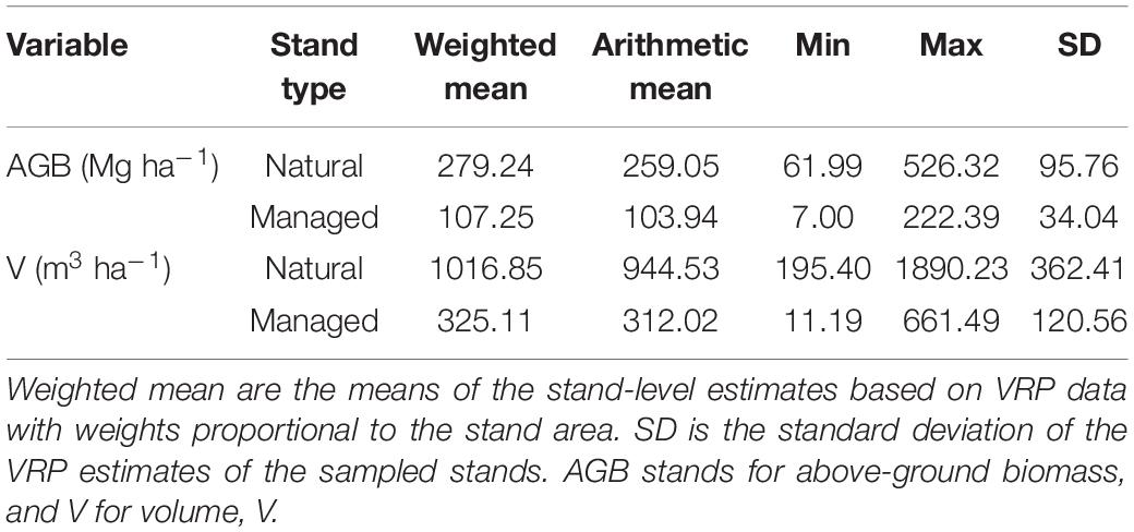
Table 1. Summary of stand-level estimates based on VRP data.

The HT estimator is unbiased and each VRP is assumed to provide an independent sample drawn under a sampling design that remains constant for all VRP in the stand. Thus, for a given stand, all ${\widehat{\mathrm{\mu }}}_{gij}$ were considered to be realizations of a random variable with mean μ_i and unknown variance ${\mathrm{\sigma }}_{ei0}^2$. The final direct estimate for the stand, ${\widehat{\mathrm{\mu }}}_{gi*}$, is the average of n_i independent and identically distributed random variables. Therefore, ${\widehat{\mathrm{\mu }}}_{gi*}$ is also a random variable with mean μ_i and its variance, ${\mathrm{\sigma }}_{ei}^2$ equals $\frac{{\mathrm{\sigma }}_{ei0}^2}{n_i}$. This allows establishing the following relation, equation 5, between the stand estimate ${\widehat{\mathrm{\mu }}}_{gi*}$, the unknown parameter of interest μ_i and the sampling error e_i

For any two stands, sampling errors are assumed to be independent of each other. Furthermore, due to the unbiasedness property of the HT estimator, errors are assumed to be distributed with zero mean and variance ${\mathrm{\sigma }}_{ei}^2$. The variance ${\mathrm{\sigma }}_{ei0}^2$ is unknown, but an unbiased estimator can be obtained pooling together the estimates of all VRP in a given stand as

Based on equation 6 the variance and the mean square error of ${\widehat{\mathrm{\mu }}}_{gi*}$ is estimated using

Estimators in equations 4, 7 are typically used in stand-level inventories using only ground data when reporting estimates and measures of uncertainty for sampled stands.

Stand-Level Fay–Herriot Models and Estimators

Stand-Level Fay–Herriot Models

Stand-level FH models explicitly acknowledge that the stand-level information on the parameter of interest is subject to sampling errors. The first component in an FH model postulates a relation between the true and unknown parameters of interest for stands and the available auxiliary information through a regression model

In equation 8, v_i is the model error that is assumed to be normally distributed with mean 0 and variance ${\mathrm{\sigma }}_v^2$ [i.e., $v_{i}N(0,{\mathrm{\sigma }}_v^2)$], β is a vector of model coefficients where the first element is the model intercept and x_i is a vector of stand-level auxiliary variables where the first element equals 1 when β includes an intercept term (see sections “Case 1: Fay–Herriot Models for New Inventories” and “Case 2: Fay–Herriot Models to Update Inventories” for a description of the auxiliary variables used for Case 1 and Case 2, respectively). These models cannot be fit because the true values of μ_i are unknown. In practice, only the direct ground estimates ${\widehat{\mathrm{\mu }}}_{gi.}$ are available, however, both, μ_i and ${\widehat{\mathrm{\mu }}}_{gi*}$ are related through the sampling model indicated in equation 5. When the regression model (8) and the sampling model (5) are combined, assuming that v_k and e_l are independent for all k and l, we obtain the basic FH model (9)

Fay–Herriot models explicitly acknowledge the presence of the sampling errors and require information on the variances ${\widehat{\mathrm{\sigma }}}_{ei}^2$ of the direct ground estimates. These variances can be estimated from the VRP data, equation 7, and then used with the known auxiliary information for the stands ${\mathbf{\text{x}}}_i^t$ and the direct estimates ${\widehat{\mathrm{\mu }}}_{gi.}$ to estimate the remaining model parameters, i.e., β and ${\mathrm{\sigma }}_v^2$. These models are typically fit using restricted maximum likelihood, REML, under the implicit assumption that sampling errors are normally distributed, i.e., $e_i\sim N(0,\frac{{\mathrm{\sigma }}_{ei0}^2}{n_i}$).

Fay–Herriot Estimators

Once FH models are fitted, they can be used to obtain stand-level estimates and their corresponding uncertainty metrics. For sampled stands, estimates based on the FH model, ${\widehat{\mathrm{\mu }}}_{FH,i}$, are obtained using the empirical best linear unbiased predictor, EBLUP,

For unsampled stands and stands with only one VRP, estimates, ${\widehat{\mathrm{\mu }}}_{FH,i}$, are obtained as synthetic estimates entirely based on the fitted model

For sampled stands, the EBLUP, equation 10, is a weighted average of the direct estimator obtained using only the ground information and the synthetic estimator. The weight and the degree of shrinking of ${\widehat{\mathrm{\mu }}}_{FHi}$ toward the synthetic estimator ${\mathbf{\text{x}}}_i^t\widehat{\mathrm{\beta }}$, is controlled by the parameter

in the following manner. For stands where the direct estimates are reliable and have small errors compared to the unexplained variance of the fitted models (i.e., ${\widehat{\mathrm{\sigma }}}_v^2>{\widehat{\mathrm{\sigma }}}_{ei}^2$), γ_i is close to 1, and ${\widehat{\mathrm{\mu }}}_{FH,i}$ is approximately equal to the ground estimate for the stand. That is, in stands with low sampling errors, the direct ground estimate is “trusted” more than the model and ${\widehat{\mathrm{\mu }}}_{FHi}\cong {\widehat{\mathrm{\mu }}}_{gi*}$. For stands where direct estimates are unreliable, ${\widehat{\mathrm{\sigma }}}_v^2={\widehat{\mathrm{\sigma }}}_{ei}^2$ the parameter γ_i is close to 0, and most weight and confidence will be put in the synthetic prediction ${\widehat{\mathrm{\mu }}}_{FH\text{s}i}\cong {\mathbf{\text{x}}}_i^t\widehat{\mathrm{\beta }}$. For unsampled stands or stands with only one VRP, γ_i cannot be computed because it is not possible to obtain the variance of the direct estimator, ${\widehat{\mathrm{\sigma }}}_{ei}^2$, with less than two VRP. Therefore, for stands with less than two VRP, all weight needs to be put in the model, and then the stand-level estimates based on the FH model are synthetic.

For stands with two or more VRP, for models fitted using REML, an approximately unbiased estimator of the mean square error of ${\widehat{\mathrm{\mu }}}_{FHi}$ is

This mean square error estimator has three components $g_1\left({\widehat{\mathrm{\sigma }}}_v^2\right)$, $g_2\left({\widehat{\mathrm{\sigma }}}_v^2\right)$, and $2g_3\left({\widehat{\mathrm{\sigma }}}_v^2\right)$ indicated in equations 14–16:

The term $\overline{V}\left({\widehat{\mathrm{\sigma }}}_v^2\right)$ in equation 15 is the inverse of the Fisher information matrix for the model (9). Details on $\overline{V}\left({\widehat{\mathrm{\sigma }}}_v^2\right)$ can be found in Rao and Molina (2015, p. 136). This estimator has a bias whose order of magnitude is o(m⁻¹), where m is the number of sampled stands. Thus in applications where a large number of stands are sampled it can be expected to provide almost unbiased estimates of the mean square error of ${\widehat{\mathrm{\mu }}}_{FHi}$. For unsampled stands or stands with only one plot, an estimator of the mean square error of ${\widehat{\mathrm{\mu }}}_{FHi}$ can be obtained using equation 17 (Rao and Molina, 2015, p. 139)

Note that we only use the subindexes >1VRP and ≤1VRP in equations 10, 11, 13, 17 to explicitly state the formulas to use depending on the number of VRP in the stand. In the remaining sections these subindexes will be omitted to simplify the notation; and ${\widehat{\mathrm{\mu }}}_{FHi}$ and $mse\left({\widehat{\mathrm{\mu }}}_{FHi}\right)$ will refer to the estimator and mse estimator needed depending on the number of VRP in the stand. The root mean square error,rmse, and relative root mean square error, rrmse, for estimates based the FH models were computed as $rmse\left({\widehat{\mathrm{\mu }}}_{FHi}\right)=\sqrt{mse\left({\widehat{\mathrm{\mu }}}_{FHi}\right)}$ and $rrmse\left({\mathrm{\mu }}_{FHi}\right)=\frac{rmse\left({\widehat{\mathrm{\mu }}}_{FHi}\right)}{{\widehat{\mathrm{\mu }}}_{FHi}}$, respectively.

Comparisons Between Fay–Herriot Estimators and Ground-Based Estimators

Comparisons between models for Case 1 and Case 2 for a given variable were based on the ratio of the estimated model variances ${\widehat{\mathrm{\sigma }}}_{vcase\mathrm{\hspace{0.25em}2}}^2/{\widehat{\mathrm{\sigma }}}_{vcase\mathrm{\hspace{0.25em}1}}^2$. To compare the uncertainty of stand-level estimates from the FH models, we used both $rmse\left({\widehat{\mathrm{\mu }}}_{FHi}\right)$ and rrmse(μ_FHi). Finally, improvements with respect to estimates based only the field data were measured using the relative efficiency. This metric was only computed for stands with two or more VRP.

Models for Case 1 and Case 2

Case 1: Fay–Herriot Models for New Inventories

For the first case scenario, auxiliary variables were computed from a recent lidar data collection completed in the fall of 2016. The lidar data were acquired using a Leica ALS70-HP lidar system mounted on a fixed-wing platform flying at an average altitude of 1965 m above the ground level with a nominal speed of 110 knots. The scanning angle was 30°, and the nominal pulse density 4.2 pulses per m².

A 30 m resolution grid was cast over the study area and lidar metrics including (1) percentiles and summaries (i.e., means, standard deviations, and moments) of the distribution of elevations above the ground of the lidar returns, (2) proportions of points in different height strata, and (3) topographic metrics were computed for each pixel using FUSION (Mc Gaughey, 2019). In total 134 variables were available. For each stand, we computed the mean and standard deviation of the pixel-level values of these metrics. The result was a total of 268 (i.e., 134 means and 134 standard deviations) stand-level metrics. These stand-level metrics were considered descriptors of the stands’ structure for the FH models for Case 1.

Case 2: Fay–Herriot Models to Update Inventories

The second case scenario consists of updating an old remote-sensing-based inventory using VRP ground measurements and FH models. For this case, auxiliary variables are stand-level predictions from a previous map and Landsat-based indexes of disturbances for the period between the old map and the date for which updated estimates were sought.

For our analyses, we used the 30 m resolution AGB map developed by Fekety and Hudak (2019) for 2013 as an old remote-sensing-based inventory. This map, CMS1-AGB map hereafter, was created in the context of the NASA Carbon Monitoring System project described in Hudak et al. (2020) using a two-step process. The first step consisted of using fixed radius plots from a set of lidar acquisitions across the northwestern United States that did not include the study area, to develop traditional ABA models where AGB was expressed as a function of lidar, topographic, and climate metrics. This model was developed at a regional scale and the plots used in the training stage included forested areas with structures and species compositions that were similar to those observed in the study area. A sample of lidar predictions in those lidar acquisitions was later used to develop a regional model to predict AGB across the forested region of the northwest United States. This regional model was primarily based on a climate metrics and Landsat time-series and was used to generate annual predictions of AGB for the period 2000–2016 at a 30 m resolution (Hudak et al., 2020). Pixel level predictions from the 2013 CMS1-AGB map were aggregated at the stand level to produce stand-level means and standard deviations of AGB predictions for 2013. These values are descriptors of the state of the forest at the moment of completion of the old inventory and are not considered to be true stand values for 2013 but approximated ones that can be used as auxiliary variables for the FH models for Case 2.

To account for changes between 2013 and 2018, we introduced additional auxiliary variables potentially correlated with growth, removals, or disturbances between 2013 and 2018 in the stands of the study area. For every stand in the study area, we computed changes between 2013 and 2018, for stand-level means, standard deviations, and modes of: (1) the red, green, blue, near-infrared, and short wave infrared one and two Landsat 8 bands, (2) band ratios including the normalized difference vegetation index (Rouse et al., 1974), NDVI, and normalized burn ratio index (Key and Benson, 2006), NBR, and (3) the brightness, wetness, and greenness tasseled cap components (Kauth and Thomas, 1976). Landsat scenes used to compute Landsat predictors correspond to the worldwide reference system path-rows 45–29 and 46–29. Median values of each Landsat band for the period going from the first of June to the 30th of September of the corresponding year were obtained and used to compute the derived indexes for each year. Stand-level means, standard deviations, and modes for bands and indexes were computed and the differences between the values obtained for 2018 and 2013 were used as auxiliary variables for the FH models. Finally, for each stand, we computed the number and proportion of pixels identified as disturbed during the period 2013–2018 by the landscape change monitoring system (LCMS) map, and the average disturbance value of all pixels identified as disturbed within the stand. The identification of disturbed pixels in LCMS is based on time series analysis of Landsat images to segment spectral trajectories. Segmentations and disturbance identification are performed with an essemble of algorithms [i.e., LandTrendr (Kennedy et al., 2010), VeRDET (Hughes et al., 2017), and CCDC (Zhu and Woodcock, 2012)]. The magnitude of the disturbances were derived as 2013–2018 changes in the relativized differenced normalized burn ratio RdNBR (Miller and Thode, 2007). In total, 38 predictors were available for Case 2. Two were the mean and standard deviation of the 2013 CMS1-AGB predictions, 18 were stand level summaries of changes in Landsat bands, 15 were stand level summaries of changes in Landsat spectral indexes and the last three were the number, proportion, and average magnitude of the disturbance metrics reported by LCMS.

Model Selection

For both scenarios, the final number of auxiliary variables available for the modeling was large (i.e., 268 for Case 1 and 38 for Case 2) and a model selection step was necessary. The model selection was performed for each combination of case scenario (i.e., Case 1 vs. Case 2), stand-type (i.e., natural vs. managed), and response variable (i.e., AGB vs. V) separately. The model selection consisted of a first step in which we used an automatic variable selection approach using best subsets regression and the R-package leaps (Lumley, 2020). In this step, we directly regressed direct estimates for AGB and V against each case’s stand-level auxiliary variables to select candidate combinations auxiliary variables. Selected combinations of auxiliary variables had lengths that ranged from 1 to 6 variables. For each number of variables, the five combinations with the lowest adjusted R² when directly regressing against the direct ground estimates were kept. This resulted in a list of 30 candidate combinations of predictors for each case scenario, stand type, and response variable. We obtained the corresponding FH models for each candidate in these lists using the R package sae (Molina and Marhuenda, 2015) using REML. Finally, the modeler selected the model to use for each case scenario, stand type and response variable, based on the estimated model error variance, ${\widehat{\mathrm{\sigma }}}_v^2$, the significance of the $\widehat{\mathrm{\beta }}$ coefficients, the Bayesian information criterion, BIC, and predicted vs. observed diagrams.

Results

Selected Models

Different patterns were observed regarding the selected models for Case 1 and Case 2 and for natural and managed stands. Regardless of the case and variable of interest, residuals for both cases tended to be centered around zero, and no significant departures with respect to the model assumptions were observed. The variability of these residuals was substantially larger for natural stands than for managed stands. Models for Case 2 tended to provide a shorter range of predicted values when compared with the models for Case 1 (Figure 4). In general, models for natural stands had a smaller number of predictors. This result was expected. The number of sampled stands is substantially smaller for natural stands than for managed stands, therefore estimated model coefficients for natural stands tend to have larger standard errors and less coefficients appeared as significant in the fitted models. The intercepts for models for natural stands for Case 1 were not significant and were removed. For both managed and natural stands, models for Case 1 had lower values of ${\widehat{\mathrm{\sigma }}}_{\mathbf{v}}^{\mathbf{2}}$. For managed stands, ${\widehat{\mathrm{\sigma }}}_{\mathbf{v}}^{\mathbf{2}}$ for AGB and V of the FH models for Case 2 were 26 and 42% larger than ${\widehat{\mathrm{\sigma }}}_{\mathbf{v}}^{\mathbf{2}}$ for Case 1, respectively. For natural stands, we observed a 4.14 and 3.27-fold increase in ${\widehat{\mathrm{\sigma }}}_{\mathbf{v}}^{\mathbf{2}}$ for AGB and V when comparing the values obtained for Case 2 with those obtained for Case 1 (Tables 2, 3). This indicates FH models based on a recent lidar acquisition explain more variance than the models for Case 2 (Tables 2, 3). When comparing models for managed and natural stands obtained under a given case scenario, we observed that for Case 1, ${\widehat{\mathrm{\sigma }}}_{\mathbf{v}}^{\mathbf{2}}$ for AGB and V in natural stands was 2.35 and 3.48 times larger than in managed stands, respectively. For Case 2, models for natural stands explained almost no variance, and for AGB and V, ${\widehat{\mathrm{\sigma }}}_{\mathbf{v}}^{\mathbf{2}}$ was 7.73 and 8.02 times larger than the one obtained in managed stands.

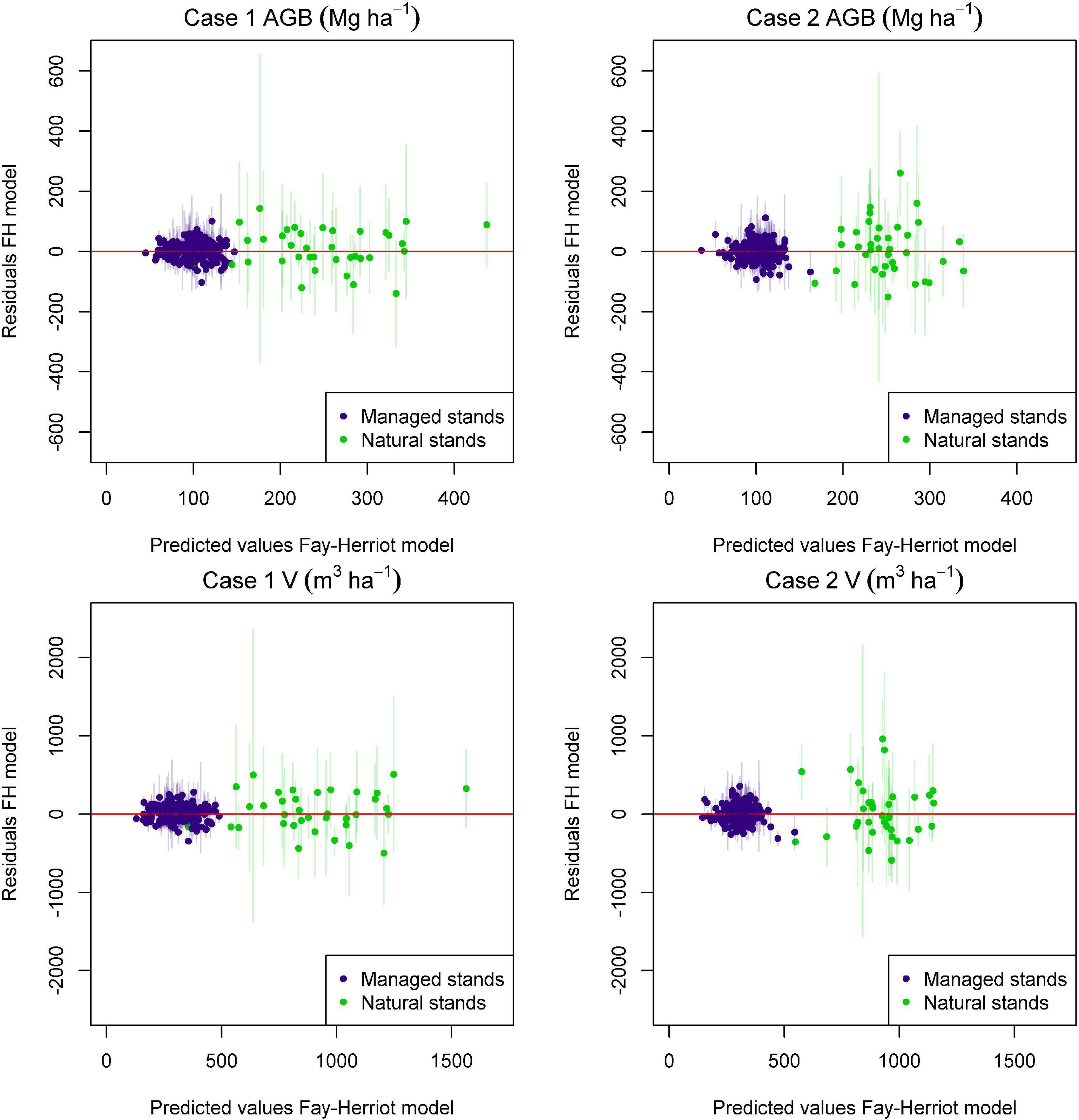
Figure 4. Predicted vs. residuals plots for FH models for above-ground biomass (AGB) and volume (V) for Case 1 and Case 2. Whiskers around each point with a width of 1.96 times the standard deviation of the direct ground estimate are included to reference the uncertainty of the field estimates associated with each data point. Residuals were computed as ${\widehat{\mathrm{\mu }}}_{\mathit{gi}*}-{\mathbf{\text{x}}}_{\mathbf{i}}^{\mathbf{t}}\widehat{\mathrm{\beta }}$, with ${\widehat{\mathrm{\mu }}}_{gi*}$ the direct ground estimate for the stand and ${\mathbf{\text{x}}}_{\mathbf{i}}^{\mathbf{t}}\widehat{\mathrm{\beta }}$ prediction entirely based on the model (prediction before computing the EBLUP).

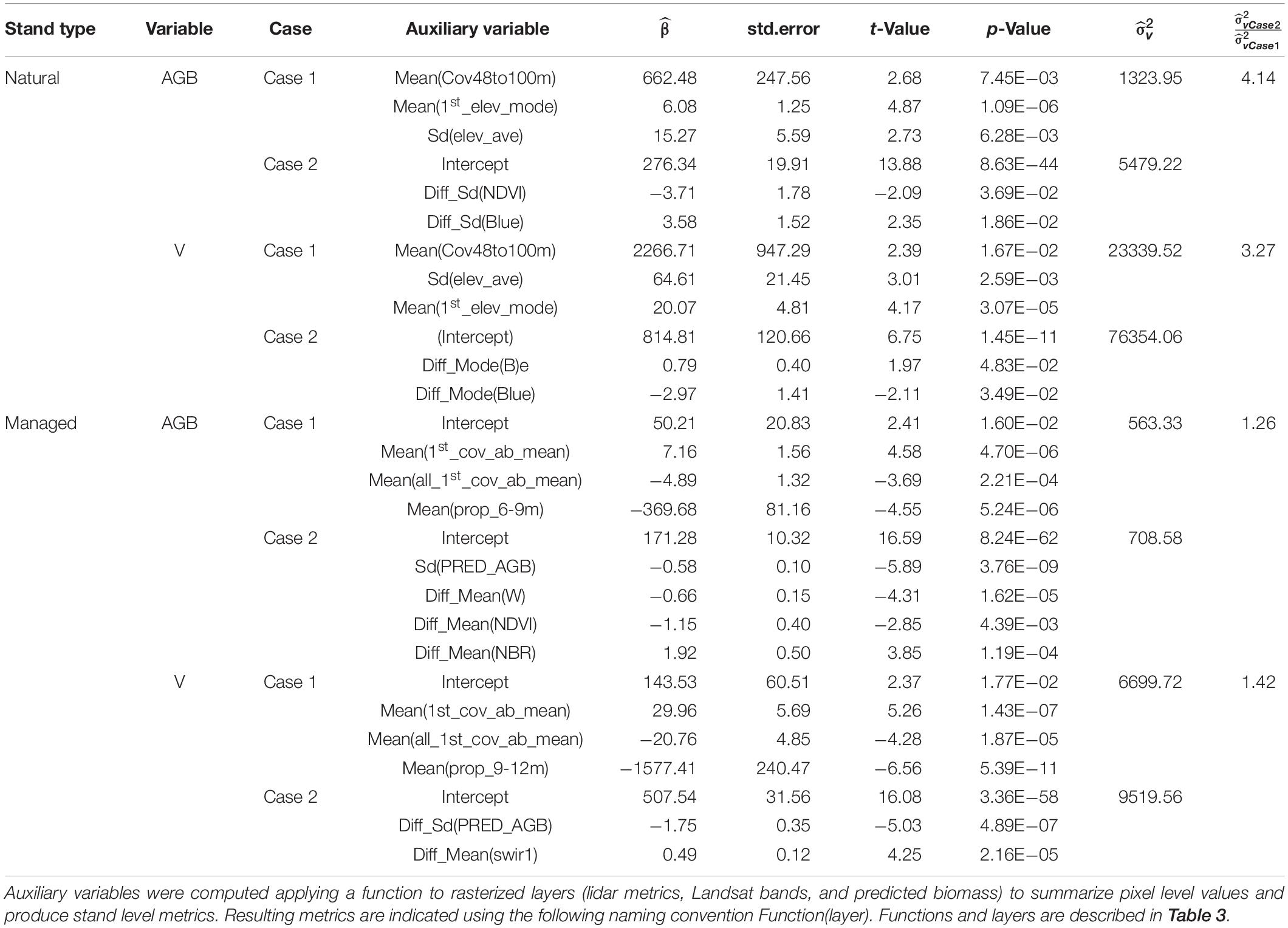
Table 2. Summary of selected models for Case 1 and Case 2 for above-ground biomass, AGB (Mg ha^–1), and volume, V (m³ ha^–1).

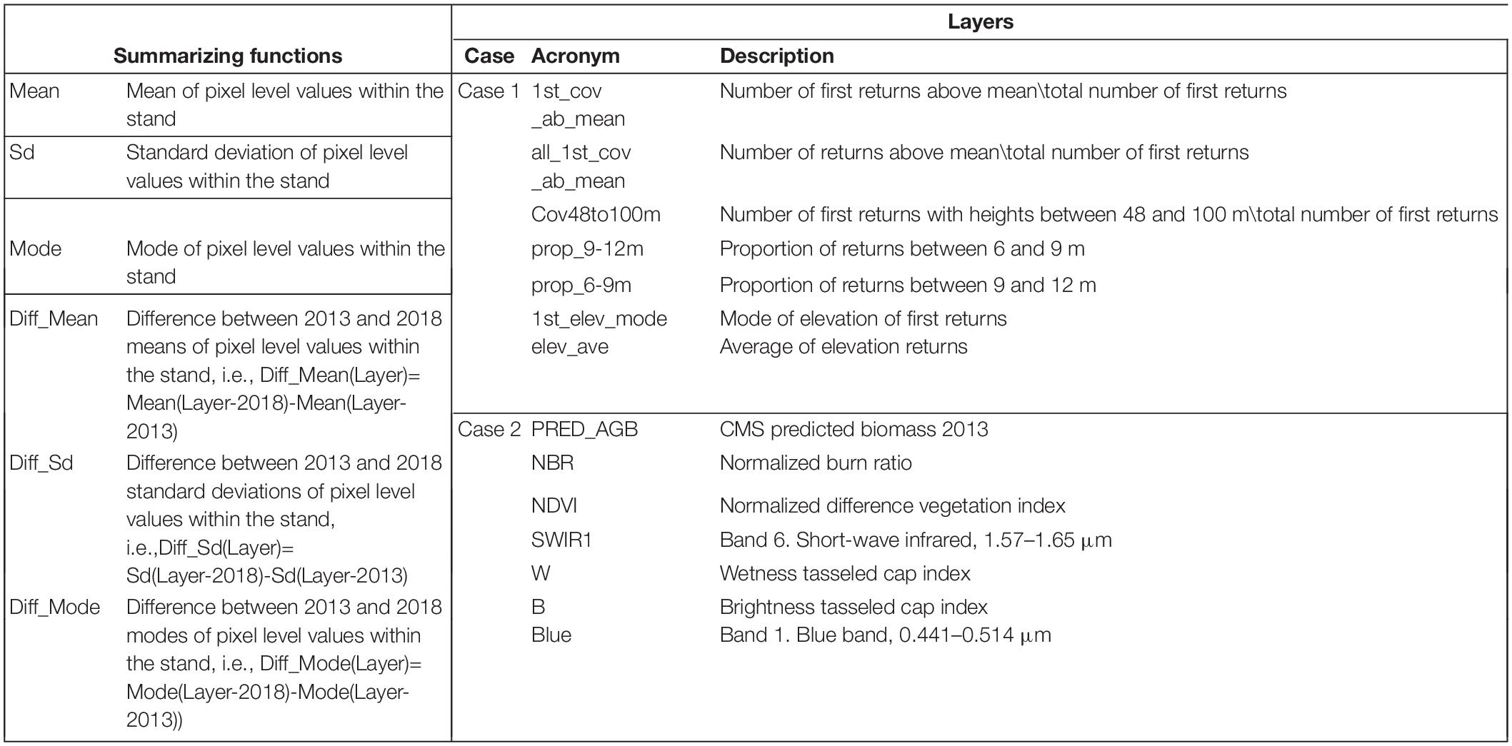
Table 3. Stand-summarizing functions applied to the 30 m resolution layers of auxiliary variables and description of metrics included in the selected models.

Stand Level Estimates

Selected models for Case 1 and Case 2 were used to obtain stand-level estimates and their associated mean squared errors for sampled and unsampled stands (Figure 5). For both cases and response variables, estimates based on FH models for managed stands tended to be smaller than estimates for natural stands and the same pattern was observed for the corresponding rmse (Figure 5). When considering rrmse, managed stands showed larger relative uncertainties. This is partly caused by the fact that managed stands stock substantially less AGB and V.

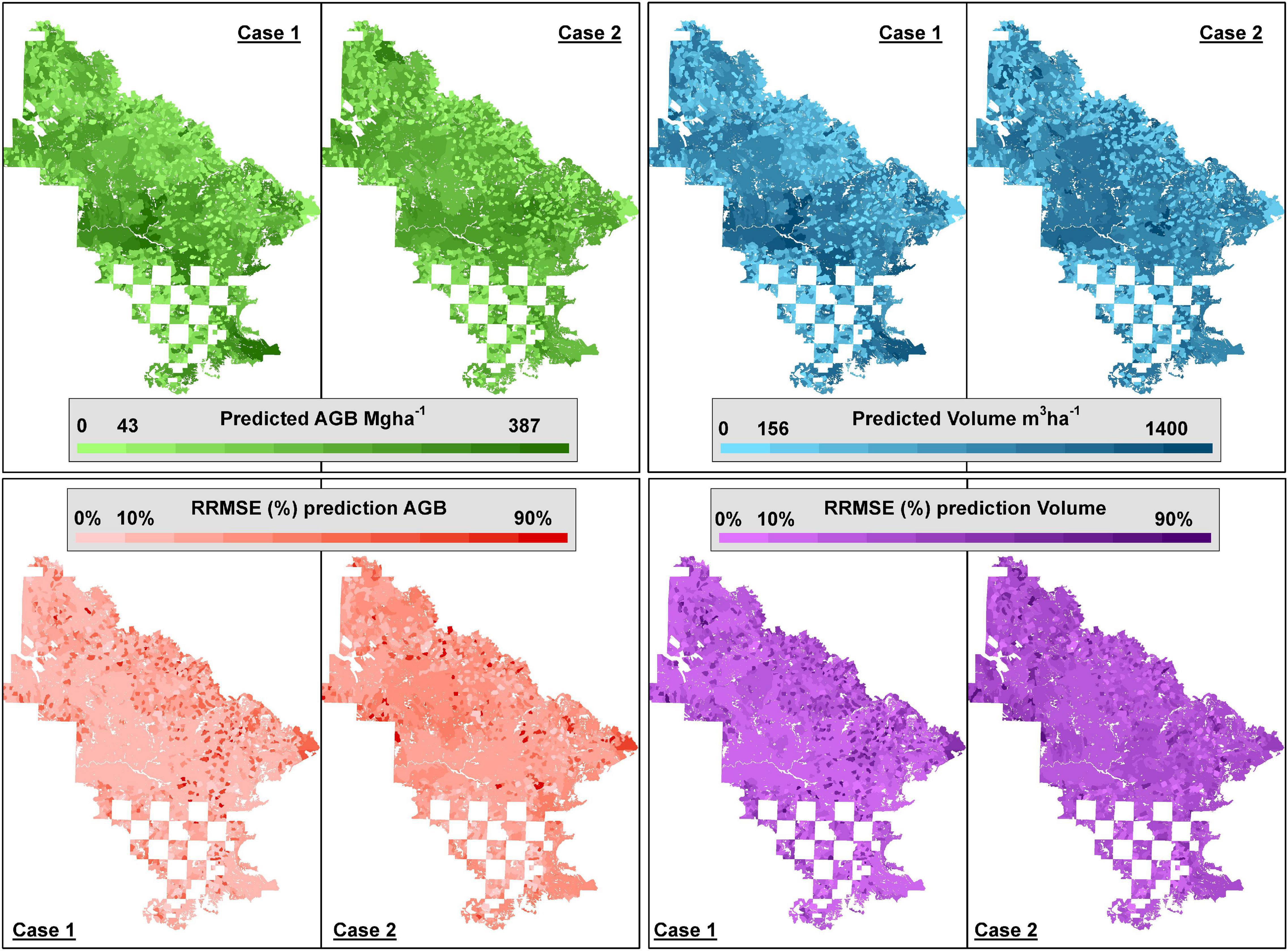
Figure 5. Stand-level predictions of above-ground biomass (AGB) and volume (V) for all stands in the study area (sampled and unsampled) and stand-level RMSE based on the FH models for Case 1 and Case 2.

For both AGB and V, estimates and rrmse obtained for Case 1 tended to agree spatially with estimates and rrmse for Case 2 (Figure 5). For natural stands, Spearman rank correlation between estimates for Case 1 and Case 2 was 0.22 (p-value = 1.04 × 10^–8) for AGB and 0.12 (p-value = 1.39 × 10^–3) for V. The low agreement for natural stands seems to be caused by the low explanatory power of the models for Case 2 in natural stands. For managed stands, Spearman rank correlation between estimates for Case 1 and Case 2 were 0.69 (p-value < 10^–6) for AGB and 0.50 (p-value < 10^–6) for V, and when each map was grouped into 10 deciles, these categories tended to coincide. The same occurred with the estimated rmse maps (see Supplementary Figure 1).

Efficiency Improvements in Sampled Stands

For both types of stands, FH models for Case 1 and Case 2 provided improvements for direct ground estimates for AGB and V. Estimates from Case 1 were consistently more precise than those from Case 2 (Figure 6). This result was expected after observing the values obtained for ${\widehat{\mathrm{\sigma }}}_v^2$ for the different models. In general, improvements in efficiency and differences between cases were larger for natural stands (Figure 6). For natural stands, improvements in efficiency for Case 1 had an average △_effi of 37.36% for AGB and 33.10% for V (Table 4). For Case 2, the average of △_effi was 20.19% for AGB and 19.25% for V. For managed stands, the average of △_effi for Case 1 was 20.29% for AGB and 19.91% for V, and for Case 2, the average of △_effi was 17.55% for AGB and 16.05% for V (Table 4). The smaller values of △_effi in managed stands is explained by the larger homogeneity of this type of stands for which many of the direct ground estimates were already precise, leaving little room for improvements to the FH models. Differences in △_effi between cases for managed stands were smaller than the differences for natural stands. This seems to be the consequence of both the low explanatory power of the auxiliary variables for Case 2 in natural stands and the smaller room for improvements in managed stands.

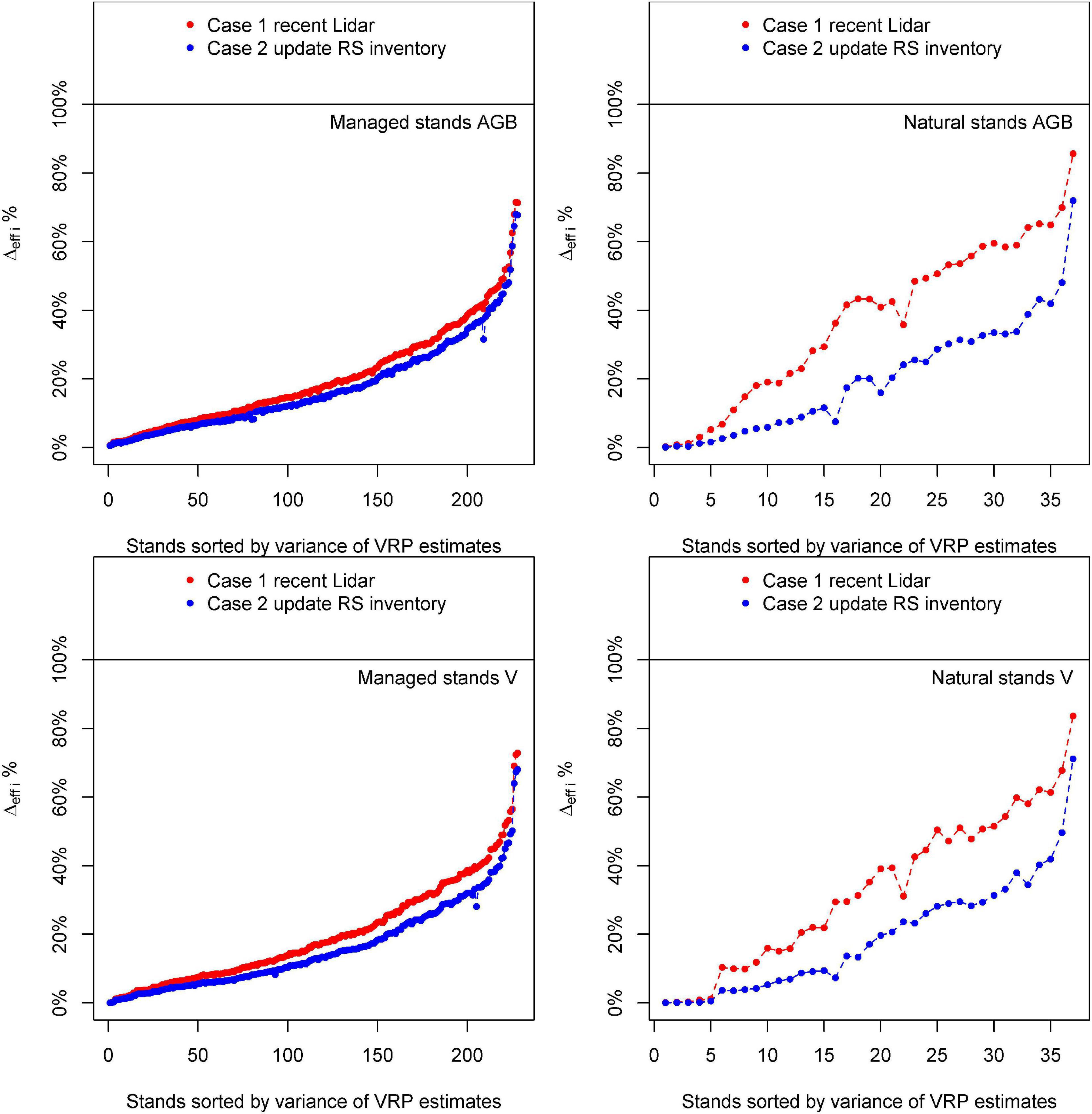
Figure 6. Reduction of uncertainty achieved by Fay–Herriot models with respect to an inventory based only on ground data(△_effi) for Case 1 and Case 2 for above-ground biomass (AGB) and volume (V).

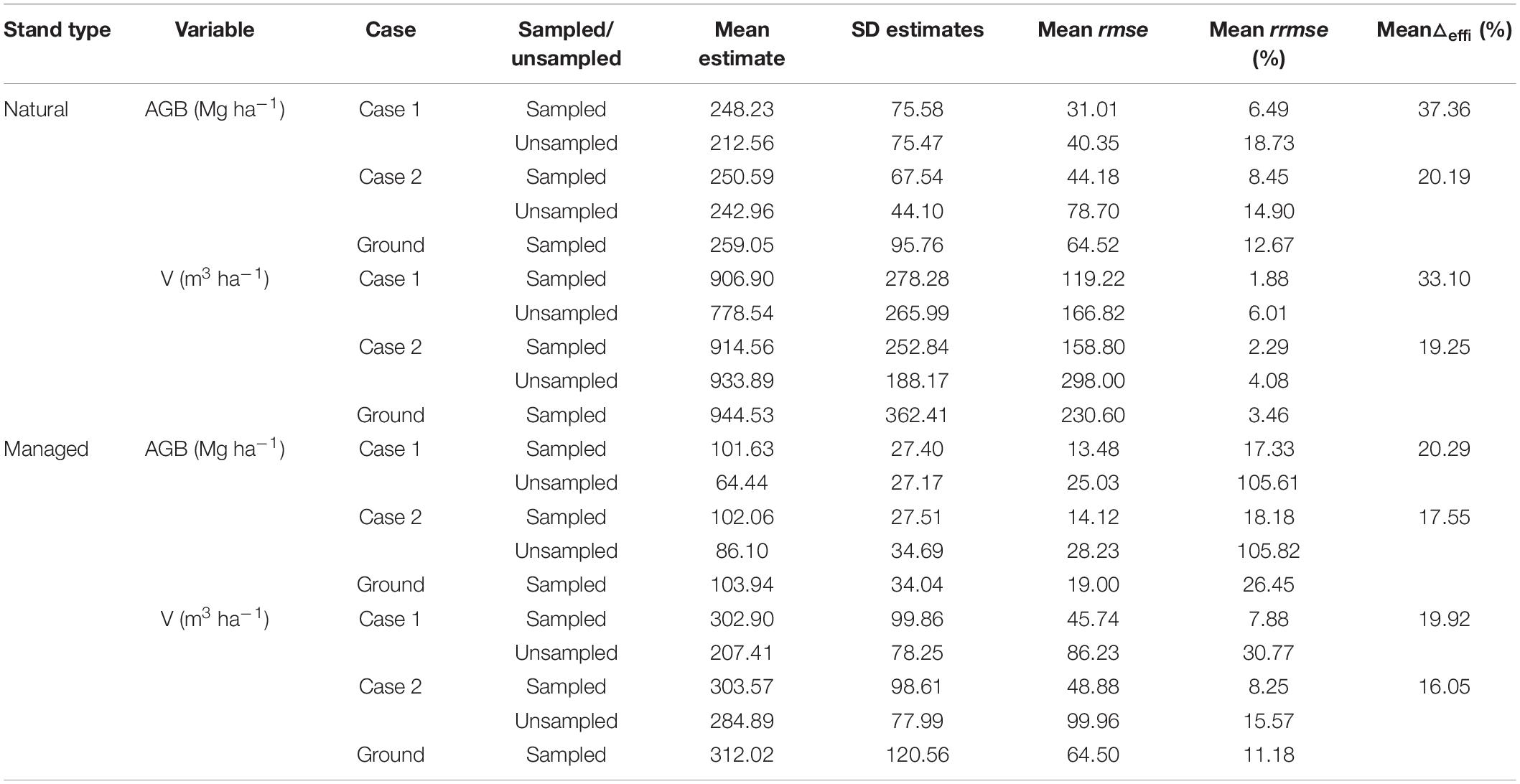
Table 4. Summary of stand-level estimates, uncertainties, and improvements in efficiency for FH models by type of stands (i.e., natural vs. managed stands), response variable (i.e., above-ground biomass, AGB, and volume, V), and case scenario (i.e., Case 1 and Case 2).

Discussion

This study presents and analyzes two possible case scenarios where FH models can be used to assist forest inventories with remote sensing information. We compared results for different stand typologies and case scenarios. We start this section by discussing the differences between cases and stand typologies and then address general issues related to the use of FH models in forest inventories.

Differences Between Case 1 and Case 2

When both scenarios were compared, estimates for Case 1 had, in general, lower errors than estimates from Case 2. The differences between cases were more important for natural stands than for managed stands. Multiple studies have shown that forest structural attributes correlate better with lidar auxiliary information than auxiliary variables from optical sensors. Auxiliary information for Case 1 proceeded from lidar. For Case 2, we used a previous remote sensing-based inventory the CMS1-AGB map, which heavily relies on metrics derived from 30-year climate normals, topographic, and Landsat variables, to which we added proxies for disturbances directly derived from Landsat images. This explains that Case 1 outperforms Case 2 for all response variables and stand types. Nevertheless, estimates from Case 2 are more efficient than direct ground estimates and regardless of the case, the rank correlations between estimates for Case 1 and Case 2 for managed stands indicated that both methods agree in the way the sort stands according to the predicted AGB or V. These results indicate that Case 2 is also useful for managed stands, and that certain management decisions, for example, concentrating harvest activities in the 10% of the managed stands with more volume, would tend to coincide regardless of which map (i.e., Case 1 or Case 2) is used to inform those decisions (see Supplementary Figure 1).

Two remarks should be made about the initial map for Case 2. On the one hand, the CMS1-AGB map has spatial and temporal coverage that cannot be matched by previous maps based only on lidar. Thus, this map can be used to develop similar stand-level inventories anywhere in the western United States. Furthermore, the multitemporal component of this map allow for possible applications of FH models to estimate changes and monitor vegetation dynamics that are not an option using single date lidar data. On the other hand, the CMS1-AGB map is expected to provide predictions with more noise than similar maps based on the ABA method and lidar data. This implies that results obtained in this study for Case 2 might improve substantially when the previous inventory is an ABA lidar-based inventory. Many countries have developed nationwide lidar acquisitions or are on the verge of completing such data collections, and national forest inventories can provide the necessary fixed area plots to use the ABA to develop maps based on lidar at national or regional scales. The effort required to develop these maps is large, and re-mapping is not expected to happen with a high frequency. This indicates that a potential niche of application of FH models and Case 2 is updating national or regional level ABA maps.

Differences Between Natural and Managed Stands

When comparing natural and managed stands, we observed that the former had larger estimated model variances, resulting in stand-level estimates with larger uncertainties in absolute terms. These differences are explained by the fact that natural stands are inherently more complex and variable than managed stands. Part of that complexity is not captured by predictors computed at the stand level. Relative uncertainties (i.e., rmse) were lower for natural stands than for managed stands. The higher stocking levels cause that in natural stands. Improvements in efficiency for natural stands were larger than those observed for managed stands, especially for Case 1. Finally, the differences in △_effi for Case 1 and Case 2 were relatively small for managed stands (i.e., about 3% difference between average values of △_effi) but large for natural stands (i.e., approximately 15% difference between average values of △_effi). The interaction of three different factors can explain this differentiated behavior. The first is that managed stands are relatively homogeneous units, and their direct ground estimates were more reliable than those obtained in natural stands. Thus, the potential for improved managed stands was more limited and made differences between cases smaller. Another factor is that the larger stocking levels are frequently associated with remote sensing predictions with larger uncertainties (Magnussen et al., 2014; Mauro et al., 2016; Breidenbach et al., 2018). Large uncertainties in the previous inventory must result in a poorer characterization of the initial state of the stands, which partially explains the performance drop for Case 2 in natural stands. The auxiliary information for Case 2 is primarily based on metrics derived from 30-year climate normals to capture steep AGB (and V) gradients, which largely compensated for signal saturation of Landsat variables (Hudak et al., 2020), albeit without sensitivity to local variation in stand structure. On the other hand, the lidar data used for Case 1 neither saturates in forested areas with closed canopies nor is insensitive to structure variation between or within stands, thus elevating the performance of the FH models for Case 1 compared to Case 2.

General Considerations for the Use of Fay–Herriot Models in Forest Inventories

For all cases, response variables and stand types analyzed in this study, FH models allowed for gains in efficiency with respect to direct ground estimates. These results are concurrent with previous research using FH models in forest inventories (Goerndt et al., 2011; Magnussen et al., 2017; Mauro et al., 2017; Breidenbach et al., 2018; Ver Planck et al., 2018) and confirm that FH models: (1) allow using ground measurements that are easier to obtain than those used in ABA approaches and (2) results in efficiency improvements when compared to methods based only on ground data. Thus, while research efforts on using FH models are still necessary, there is substantial evidence that these models can play an essential role in operational forest inventory applications.

To the best of our knowledge, FH models have not been used in any operational forest inventory, and it somehow surprises how little attention FH models have received in the literature. While some research applications of FH models exist, the study of this type of model has been negligible compared to applications using conventional ABA approaches. The dominance of the traditional ABA approach can be explained by (1) its ability to produce high resolution maps with predictions of forest attributes and (2) its typically better predictive performance than FH models (Mauro et al., 2017; Breidenbach et al., 2018; Green et al., 2019). However, developing ABA models is not always a possibility. There are many scenarios where FH models can be a very appealing alternative; for example, only stand-level inventory data may be available. During the last decades, forest inventories have been consistently less constrained by the availability of useful auxiliary information, but the costs associated with ground data collection have increased, or at least not decreased at comparable rates. Simply put, ground data are too valuable to ignore, and FH models allow for an effective combination of those valuable datasets with different sources of auxiliary information.

A critical difference between traditional ABA models and FH models is the auxiliary information used by each technique. Workflows for preprocessing auxiliary information for traditional ABA models are well established and documented, with multiple tools available to implement these processing steps (i.e., Mc Gaughey, 2019; Roussel et al., 2020); this is not the case for FH models. In this study, we used as predictors stand summaries of: (1) gridded products (i.e., gridmetrics rasters) generated with FUSION (Mc Gaughey, 2019), (2) previously mapped estimates of forest attributes, and (3) changes in Landsat imagery from LCMS or computed using Google earth engine (Gorelick et al., 2017). Summarizing the entire point clouds within the stands under analysis is an alternative used in previous studies to compute lidar-based predictors (Ver Planck et al., 2018). Both options are valid from a methodological perspective as they provide standardized ways to compute auxiliary variables. Their effectiveness can differ if one preprocessing technique provided auxiliary variables that correlated better with the target responses than the other. However, as far as we know, no study to date has analyzed the differences in performance and tradeoffs of these two methods to generate stand-level predictors for FH models. Thus, this is an area where future research can help in establishing standardized processing workflows for lidar-assisted forest inventories using FH models.

This study presents two case scenarios in which basic FH models are used with VRP and demonstrates that FH models are a suitable alternative to use available auxiliary information to improve the efficiency of the estimation process. Our analysis presents a baseline for stand-level FH models and could be improved in different ways. One way is developing models that account for spatial correlations like those developed by Ver Planck et al. (2018). Another option is to use FH variants where the model variance is not constant (Breidenbach et al., 2018). A third option is to use multivariate FH models where correlations between different response variables can be considered to improve the results of univariate models (Benavent and Morales, 2016; Frank, 2020). In all cases, one factor that must be constantly considered is that estimates obtained from FH models are always based on a model (i.e., “model-based”). Thus, extrapolations entail high risks of producing biased estimates and model validation steps are critical to ensure that the fitted models correctly describe the populations under study.

Based on our findings and previous results (Goerndt et al., 2011; Breidenbach et al., 2018; Ver Planck et al., 2018), we envision that niche of application of stand-level FH models is not a replacement of traditional ABA methods but a complement for situations in which the time and resources available for ground data collection are limited or fixed radius plots with precise locations to develop ABA models are otherwise unavailable. This niche is larger than it might seem a priori for several reasons. One reason is that obtaining accurate coordinates for the ground measurements is not a constraint for FH models. For example, only the identifier of the stand where each ground observation was taken was necessary to develop this study using FSVeg data. Another reason, and probably the most compelling one, is that FH models can be applied with data from VRP or other sampling techniques such as sector plots (Iles and Smith, 2006) or transects (Warren and Olsen, 1964; Woodall and Monleon, 2008). This flexibility indicates numerous applications for fast inventories and monitoring problems in which FH models can be the preferred alternative. These applications include, but are not limited to, annual inventories for timber sales or fast updates of inventories after events like floods or wildland fires.

Improved AGB and V benefit both private companies and public land management agencies. Given the extremely high cost of establishing ground plots and the increasing demand for accurate biomass and carbon stock assessment, the inventory solution will require the innovative use of combined sources of remotely sensed and other auxiliary data. FH models based on VRP allow using remotely sensed information combined with an operative ground truth data collection and enable cost-effectively estimating forest attributes. In this study, the FH models have shown to be a viable and flexible option to estimate AGB or V and maximize the utility of both the ground inventory and environmental datasets. Moreover, different information for forest management planning is required at different levels or scales. For tactical planning, reasonably precise and unbiased estimates of forest variables for individual stands or polygons are already obtained using VRP because of its low cost and sampling efficiency at the stand level. Thus, FH models are an alternative for many established inventory programs to integrate their VRP data with lidar or other remote-sensing datasets to obtain more efficient and better information for sustainable forest management.

Conclusion

The main conclusion obtained when comparing estimates from FH models for Case 1 and Case 2 indicated that estimates from FH models based on a recent lidar acquisition were the most efficient alternative. For managed stands, differences between case scenarios were small, but in natural stands, FH models based on data from a recent lidar data collection produced more efficient results substantially. However, in all cases, estimates from FH models for both case scenarios and both types of forest stands were more efficient than direct ground estimates. Based on this result, we conclude that FH models are a valuable alternative for many forest inventory tasks if fixed area plots or their precise geolocations are unavailable.

Data Availability Statement

The datasets presented in this article are not readily available because this study was developed using data from Field Sampled Vegetation (FSVeg) database. USDA Federal employees, contractors, and affiliates need to follow the steps indicated in the link below to access the data. https://www.fs.fed.us/nrm/documents/fsveg/cse_user_guides/FSVegQuickGuide.pdf.

Author Contributions

HT wrote some parts of the manuscript, verified the analytical methods, critically reviewed the manuscript, and supervised the findings of this work. FM conceived of the presented idea, performed the computations, and wrote the first version of the manuscript. AH, BF, and VM critically reviewed the manuscript and provided critical feedback. PF, MP, and TB contributed to the final version of the manuscript. All authors discussed the results and contributed to the final manuscript.

Funding

This work was supported by Challenge Cost Share Agreement 20-CS-11062754-066 between Oregon State University and the USDA Forest Service, Pacific Northwest Region and by a NASA Carbon Monitoring System Program award (80HQTR20T0002) through a Joint Venture Agreement (20-JV-11221633-112) between the USDA Forest Service, Rocky Mountain Research Station and Oregon State University.

Conflict of Interest

The authors declare that the research was conducted in the absence of any commercial or financial relationships that could be construed as a potential conflict of interest.

Publisher’s Note

All claims expressed in this article are solely those of the authors and do not necessarily represent those of their affiliated organizations, or those of the publisher, the editors and the reviewers. Any product that may be evaluated in this article, or claim that may be made by its manufacturer, is not guaranteed or endorsed by the publisher.

Acknowledgments

We would like to acknowledge Cheryl Friesen, James Rudisill, and Karin Wolken that were an active part in discussions that led to the ideas presented in this manuscript.

Supplementary Material

The Supplementary Material for this article can be found online at: https://www.frontiersin.org/articles/10.3389/ffgc.2021.745916/full#supplementary-material

References

Babcock, C., Finley, A. O., Bradford, J. B., Kolka, R., Birdsey, R., and Ryan, M. G. (2015). LiDAR based prediction of forest biomass using hierarchical models with spatially varying coefficients. Remote Sens. Environ. 169, 113–127. doi: 10.1016/j.rse.2015.07.028
Benavent, R., and Morales, D. (2016). Multivariate Fay–Herriot models for small area estimation. Comput. Stat. Data Anal. 94, 372–390. doi: 10.1016/j.csda.2015.07.013
Breidenbach, J., Magnussen, S., Rahlf, J., and Astrup, R. (2018). Unit-level and area-level small area estimation under heteroscedasticity using digital aerial photogrammetry data. Remote Sens. Environ. 212, 199–211. doi: 10.1016/j.rse.2018.04.028
Coulston, J. W., Green, P. C., Radtke, P. J., Prisley, S. P., Brooks, E. B., Thomas, V. A., et al. (2021). Enhancing the precision of broad-scale forestland removals estimates with small area estimation techniques. Forestry 94, 427–441. doi: 10.1093/forestry/cpaa045
Deo, R. K., Froese, R. E., Falkowski, M. J., and Hudak, A. T. (2016). Optimizing variable radius plot size and LiDAR resolution to model standing volume in conifer forests. Can. J. Remote Sens. 42, 428–442.
Fay, R. E., and Herriot, R. A. (1979). Estimates of income for small places: an application of james-stein procedures to census data. J. Am. Stat. Assoc. 74, 269–277. doi: 10.2307/2286322
Fekety, P. A., Falkowski, M. J., Hudak, A. T., Jain, T. B., and Evans, J. S. (2018). Transferability of lidar-derived basal area and stem density models within a Northern Idaho Ecoregion. Can. J. Remote Sens. 44, 131–143. doi: 10.1080/07038992.2018.1461557
Fekety, P. A., and Hudak, A. T. (2019). Annual Aboveground Biomass Maps for Forests in the Northwestern USA, 2000-2016. Oak Ridge, TN: National Laboratory Distributed Active Archive Center, doi: 10.3334/ORNLDAAC/1719
Forkuor, G., Benewinde Zoungrana, J.-B., Dimobe, K., Ouattara, B., Vadrevu, K. P., and Tondoh, J. E. (2020). Above-ground biomass mapping in West African dryland forest using sentinel-1 and 2 datasets - a case study. Remote Sens. Environ. 236, 111496. doi: 10.1016/j.rse.2019.111496
Frank, B. M. (2020). Aerial Laser Scanning for Forest Inventories: Estimation and Uncertainty at Multiple Scales. Ph.D. thesis. Corvallis, OR: Oregon State University.
Frank, B., Mauro, F., and Temesgen, H. (2020). Model-based estimation of forest inventory attributes using lidar: a comparison of the area-based and semi-individual tree crown approaches. Remote Sens. 12:2525. doi: 10.3390/rs12162525
Goerndt, M. E., Monleon, V. J., and Temesgen, H. (2011). A comparison of small-area estimation techniques to estimate selected stand attributes using LiDAR-derived auxiliary variables. Can. J. For. Res. 41, 1189–1201.
González-Ferreiro, E., Diéguez-Aranda, U., and Miranda, D. (2012). Estimation of stand variables in Pinus radiata D. don plantations using different LiDAR pulse densities. Forestry 85, 281–292. doi: 10.1093/forestry/cps002
Gorelick, N., Hancher, M., Dixon, M., Ilyushchenko, S., Thau, D., and Moore, R. (2017). Google earth engine: planetary-scale geospatial analysis for everyone. Remote Sens. Environ. 202, 18–27. doi: 10.1016/j.rse.2017.06.031
Grafström, A., Schnell, S., Saarela, S., Hubbell, S. P., and Condit, R. (2017). The continuous population approach to forest inventories and use of information in the design. Environmetrics 28:e2480. doi: 10.1002/env.2480
Green, P. C., Burkhart, H. E., Coulston, J. W., and Radtke, P. J. (2019). A novel application of small area estimation in loblolly pine forest inventory. Forestry 93, 444–457. doi: 10.1093/forestry/cpz073
Hudak, A. T., Fekety, P. A., Kane, V. R., Kenedy, R. E., Filipelli, S. K., Falkowski, M. J., et al. (2020). A carbon monitoring system for mapping regional, annual aboveground biomass across the northwestern USA. Environ. Res. Lett. 15:095003.
Hudak, A. T., Haren, A. T., Crookston, N. L., Liebermann, R. J., and Ohmann, J. L. (2014). Imputing forest structure attributes from stand inventory and remotely sensed data in western Oregon, USA. For. Sci. 60, 253–269.
Hughes, M. J., Kaylor, S. D., and Hayes, D. J. (2017). Patch-based forest change detection from landsat time series. Forests 8:166. doi: 10.3390/f8050166
Hummel, S., Hudak, A., Uebler, E., Falkowski, M., and Megown, K. (2011). A comparison of accuracy and cost of LiDAR versus stand exam data for landscape management on the Malheur National Forest. J. For. 109, 267–273.
Iles, K., and Smith, N. J. (2006). A new type of sample plot that is particularly useful for sampling small clusters of objects. For. Sci. 52, 148–154. doi: 10.1093/forestscience/52.2.148
Kauth, R. J., and Thomas, G. (1976). “The tasselled cap–a graphic description of the spectral-temporal development of agricultural crops as seen by Landsat,” in Proceedings of the Machine Processing of Remotely Sensed Data, (West Lafayette, IN: Purdue University).
Kennedy, R. E., Yang, Z., and Cohen, W. B. (2010). Detecting trends in forest disturbance and recovery using yearly landsat time series: 1. landtrendr — temporal segmentation algorithms. Remote Sens. Environ. 114, 2897–2910. doi: 10.1016/j.rse.2010.07.008
Key, C. H., and Benson, N. C. (2006). “Landscape assessment (LA),” in FIREMON: Fire Effects Monitoring and Inventory System, eds D. C. Lutes, R. E. Keane, J. F. Caratti, C. H. Key, N. C. Benson, S. Sutherland, et al. (Ogden, UT: US Department of Agriculture, Forest Service, Rocky Mountain Research Station), 1–55.
LeMay, V., Maedel, J., and Coops, N. C. (2008). Estimating stand structural details using nearest neighbor analyses to link ground data, forest cover maps, and Landsat imagery. Remote Sens. Environ. 112, 2578–2591. doi: 10.1016/j.rse.2007.12.007
Lumley, T. (2020). Leaps: Regression Subset Selection. Available online at: http://CRAN.R-project.org/package=leaps. (accessed October 6, 2021).
Magnussen, S., Mandallaz, D., Breidenbach, J., Lanz, A., and Ginzler, C. (2014). National forest inventories in the service of small area estimation of stem volume. Can. J. For. Res. 44, 1079–1090. doi: 10.1139/cjfr-2013-0448
Magnussen, S., Mauro, F., Breidenbach, J., Lanz, A., and Kändler, G. (2017). Area-level analysis of forest inventory variables. Eur. J. For. Res. 136, 839–855. doi: 10.1007/s10342-017-1074-z
Maltamo, M., Eerikäinen, K., Pitkänen, J., Hyyppä, J., and Vehmas, M. (2004). Estimation of timber volume and stem density based on scanning laser altimetry and expected tree size distribution functions. Remote Sens. Environ. 90, 319–330.
Mauro, F., Molina, I., García-Abril, A., Valbuena, R., and Ayuga-Téllez, E. (2016). Remote sensing estimates and measures of uncertainty for forest variables at different aggregation levels. Environmetrics 27, 225–238. doi: 10.1002/env.2387
Mauro, F., Monleon, V. J., Temesgen, H., and Ford, K. R. (2017). Analysis of area level and unit level models for small area estimation in forest inventories assisted with LiDAR auxiliary information. PLoS One 12:e0189401. doi: 10.1371/journal.pone.0189401
Mauro, F., Ritchie, M., Wing, B., Frank, B., Monleon, V., Temesgen, H., et al. (2019). Estimation of changes of forest structural attributes at three different spatial aggregation levels in northern California using multitemporal LiDAR. Remote Sens. 11:923. doi: 10.3390/rs11080923
Mc Gaughey, R. J. (2019). FUSION\LDV: Software for LIDAR Data Analysis and Visualization. Washington, D.C: USDA Forest Service.
Miller, J. D., and Thode, A. E. (2007). Quantifying burn severity in a heterogeneous landscape with a relative version of the delta Normalized Burn Ratio (dNBR). Remote Sens. Environ. 109, 66–80. doi: 10.1016/j.rse.2006.12.006
Næsset, E. (2002). Predicting forest stand characteristics with airborne scanning laser using a practical two-stage procedure and field data. Remote Sens. Environ. 80, 88–99.
Pflugmacher, D., Cohen, W. B., and Kennedy, R. E. (2012). Using landsat-derived disturbance history (1972–2010) to predict current forest structure. Remote Sens. Environ. 122, 146–165. doi: 10.1016/j.rse.2011.09.025
Rao, J. N. K., and Molina, I. (2015). “Empirical best linear unbiased prediction (EBLUP): basic area level model,” in Small Area Estimation, ed. P. Lahiri (Hoboken, NJ: John Wiley & Sons, Inc), 123–172.
Rouse, J. W., Haas, R. H., Schell, J. A., and Deering, D. W. (1974). Monitoring vegetation systems in the Great Plains with ERTS. NASA special publication 351, 309.
Roussel, J.-R., Coops, N. C., Tompalski, P., Goodbody, T. R. H., Meador, A. S., Bourdon, J.-F., et al. (2020). lidR: an R package for analysis of airborne laser scanning (ALS) data. Remote Sens. Environ. 251:112061. doi: 10.1016/j.rse.2020.112061
Vafaei, S., Soosani, J., Adeli, K., Fadaei, H., Naghavi, H., Pham, T. D., et al. (2018). Improving accuracy estimation of forest aboveground biomass based on incorporation of ALOS-2 PALSAR-2 and sentinel-2A imagery and machine learning: a case study of the hyrcanian forest area (Iran). Remote Sens. 10:172. doi: 10.3390/rs10020172
Ver Planck, N. R., Finley, A. O., Kershaw, J. A., Weiskittel, A. R., and Kress, M. C. (2018). Hierarchical Bayesian models for small area estimation of forest variables using LiDAR. Remote Sens. Environ. 204, 287–295. doi: 10.1016/j.rse.2017.10.024
Warren, W. G., and Olsen, P. F. (1964). A line intersect technique for assessing logging waste. For. Sci. 10, 267–276. doi: 10.1093/forestscience/10.3.267
Woodall, C., and Monleon, V. (2008). Sampling Protocol, Estimation, and Analysis Procedures for the Down Woody Materials Indicator of the FIA Program. Newtown Square, PA: Northern Research Station.
Keywords: stand-level models, lidar, above-ground biomass, carbon monitoring system, uncertainty
Citation: Temesgen H, Mauro F, Hudak AT, Frank B, Monleon V, Fekety P, Palmer M and Bryant T (2021) Using Fay–Herriot Models and Variable Radius Plot Data to Develop a Stand-Level Inventory and Update a Prior Inventory in the Western Cascades, OR, United States. Front. For. Glob. Change 4:745916. doi: 10.3389/ffgc.2021.745916
Received: 22 July 2021; Accepted: 30 September 2021;
Published: 20 October 2021.
Edited by:
Philip Radtke, Virginia Tech, United StatesReviewed by:
Johannes Rahlf, Norwegian Institute of Bioeconomy Research (NIBIO), NorwayQianqian Cao, Virginia Tech, United States
Copyright © 2021 Temesgen, Mauro, Hudak, Frank, Monleon, Fekety, Palmer and Bryant. This is an open-access article distributed under the terms of the Creative Commons Attribution License (CC BY). The use, distribution or reproduction in other forums is permitted, provided the original author(s) and the copyright owner(s) are credited and that the original publication in this journal is cited, in accordance with accepted academic practice. No use, distribution or reproduction is permitted which does not comply with these terms.
*Correspondence: Hailemariam Temesgen, temesgen.hailemariam@oregonstate.edu
†These authors share first authorship