Identifying Habitat Holdouts for High Elevation Tree Species Under Climate Change

Introduction

Climate change has caused, and will continue to cause, significant changes in tree species' distributions (Lenoir et al., 2008). Paleo-ecological studies have shown that geographical ranges of tree species across the globe have expanded and contracted since the last glacial maximum (see Svenning et al., 2015). These range shifts are, however, dependent on local context: topographic and climatic interactions result in microclimates that allow for the localized persistence of tree species that would otherwise be lost under the regional climate (Dobrowski, 2011; Keppel et al., 2012). Hannah et al. (2014) classified microrefugia based on the persistence of the climate sensitive species in that location: stepping stones are areas where the microclimate allows species to migrate through; holdouts are areas where the species can persist for some indeterminate amount of time; and microrefugia are areas where the species can persist until a favorable climate returns.

The optimal scale at which to identify holdouts is a challenge: estimates must account for scale dependent processes like competition, demographics, and disturbance in addition to climate, as all these factors are crucial for determining a species' presence (Malanson et al., 2007; Copenhaver-Parry et al., 2017). Issues of dispersal and competition can lead to climate disequilibrium whereby species fail to migrate at the rate of climate change (Svenning and Sandel, 2013). Moreover, species with a strong dispersal advantage can jump over other species to take advantage of new habitat (Smithers et al., 2018). For a microrefugium for any particular tree species to remain viable, it requires the persistence of favorable microclimate and maintenance of the disturbance regime for which the species is adapted (e.g., fire may be necessary to allow sufficient light for germination; Hannah et al., 2014). Climate change and other human factors are expected to alter these disturbance regimes, specifically fire regimes for the western US (Westerling et al., 2006).

Montane landscapes highlight the challenges for identifying holdouts. Because of their complex topography, montane landscapes offer a variety of microclimates through a combination of aspect and elevation (Bell et al., 2014a). However, throughout the western US, tree species in the montane to alpine belts have been declining in prevalence and area (Andrus et al., 2018; DeSiervo et al., 2018). This trend is expected to increase with climate change, where expected warmer temperatures will reduce soil moisture while increasing evaporative demand, resulting in drought-induced mortality and regeneration failure for more mesic species (Millar et al., 2012; Andrus et al., 2018).

Accounting for all of these processes requires a compromise between scale and resolution within existing methods and models (Levin, 1992). Species distribution models may account for climatic changes, but do not necessarily account for dynamic interactions among species, and are ultimately reliant on statistical correlations (Franklin, 2010). Stand level models, such as the Forest Vegetation Simulator (FVS) can account for competition and climatic change (e.g., Hurteau et al., 2014), but does not operate on a scale large enough to capture population movements. Dynamic global vegetation models, such as MC2, may track population movements and disturbances but lack the resolution (e.g., 30 arc-seconds—approximately 1 km—grid spacing in Kim et al., 2018) to identify microrefugia. Landscape level models, such as LANDIS, offer a compromise: climatic changes, disturbances, population movement, and competition at the species scale, allowing for the identification of potential refugia at moderate resolution.

We sought to identify holdouts, specifically areas where species can persist through 2100, within a high-conservation value montane forest. Holdouts were chosen because average temperatures are expected to increase through the end of the century and beyond. The questions we asked with this study are: (1) where on the landscape these species can persist into the future, in light of the effects of climate change on the region? (2) how does the model resolution affect species occurrence on the landscape and the ability to identify holdouts? (3) can we generalize from the modeling results to find holdouts in the larger region without relying on having to operate a computationally intensive model at a fine scale resolution? Ultimately these questions can help address a central question of the future management of or for these species: given the expected decline, what are the management options available?

Methods

Study Area

The Klamath region of northern California is an ideal area to study the persistence of microrefugia given its tree species diversity and complex geology and topography (Cheng, 2004). The diversity is the result of the presence of serpentine soils, topographic complexity, and its history as a refugium through the last glacial maximum (Whittaker, 1960). We focused on the Marble Mountain Wilderness (MMW) and the surrounding high elevation area, covering ~170,000 hectares in total (Figure 1). The MMW was designated a primitive area in 1931 and wilderness in 1964, and as a result avoids the confounding effect of recent forest management on current species distributions. It is part of a larger network of wilderness areas, with the Russian Wilderness most immediately to the southeast, which has experienced declines in high elevation tree species (DeSiervo et al., 2018). The Marble Mountains, the namesake for the wilderness, connect several mountain ranges, spanning from the Trinity Alps to the south, to the Siskiyous to the north, and through the Siskiyous to the Cascades to the northeast. The projected average temperatures of the region are expected to increase by 1 to 3°C by the end of this century, depending on climate forcing, while precipitation is expected to vary widely (−15 to +10% compared to contemporary climate) over the same time.

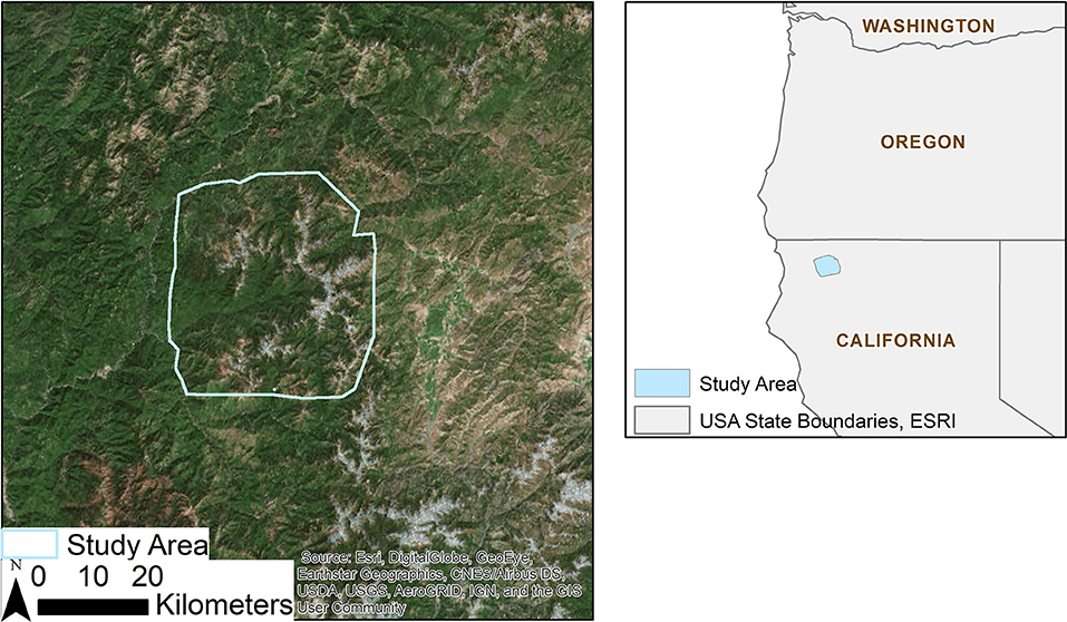
Figure 1. Map of the study area, a 190,000-hectare area in northwest California, primarily centered on the Marble Mountain Wilderness.

With over 2,000 m of topographic relief, there are several distinct belts of vegetation. Because the highest peaks are only 2,500 m above sea level (m.a.s.l.), most all are below treeline with the highest belt of vegetation being sub-alpine. The following species are representative for that belt for this region: white fir (Abies concolor (Gord. & Glend.) Lindl. ex Hildebr.), red fir (Abies magnifica A. Murr), and western white pine (Pinus monticola Dougl. ex D. Don) (Burns and Honkala, 1990). Intermixed with these species, but dominant at lower elevations is Douglas-fir (Pseudotsuga menziesii (Mirb.) Franco). White fir is close to its northern end of its range in the Klamath region though it is closely related to grand fir (Abies grandis (Douglas ex D. Don) Lindl.) to the north, dominating the mixed conifer forest type at high elevations, and transitions to red fir at higher elevations (Laacke, 1990a; Zouhar, 2001). Red fir hybridizes with California red fir (Abies procera Redher) in this region, placing populations in the Klamath in the middle of its distribution; it can become a climax species in high elevation areas unless removed by disturbance (Laacke, 1990b). Western white pine is a common component in many forest cover types; however, the species is susceptible to white pine blister rust, Cronartium ribicola, an introduced fungus that causes mortality throughout the life stages of western white pine, but especially mature trees. In the study area, A. concolor occupies ~47% of the study area, A. magnifica 22%, and P. monticola 9%. In addition, the area is home to a number of relict and endemic species. They include species found at the extreme southern end of their distribution (Alaska yellow-cedar, Callitropsis nootkatensis (D. Don) Oerst. ex D.P. Little) or endemic (Brewer spruce, Picea breweriana S. Watson) (Burns and Honkala, 1990).

Simulation Modeling

We addressed our questions using a landscape simulation approach, given the necessity of considering dynamic climate, fire regimes, and species distributions. We chose the LANDIS-II model because it emphasizes spatial interactions among processes across the landscape over many decades (Scheller et al., 2007). LANDIS-II simulates forests as species-age cohorts within raster cells, where those cohorts compete for resources, including light, water, and nitrogen, within each cell. Cohorts reproduce via seed dispersal and re-sprouting. Seed dispersal follows Ward et al. (2004), where the probability of dispersal follows a negative exponential curve with most of the distribution falling within the effective distance (Scheller et al., 2011). Regeneration is determined by soil moisture and climate, and as species move out of their ideal climate envelope the probability of successful establishment falls (Liang et al., 2017). However, drought mortality is not directly modeled. The model operates as a core module interacting with various extensions that can simulate succession, disturbances, and management. The extensions used here include Net Ecosystem Carbon and Nitrogen (NECN) Succession (v4.2.1), Dynamic Fuels and Fire (v2.2.1, see below), Dynamic Biomass Fuels (v4.0), and Biomass Output (v2.2). The same climate data were used across all processes and extensions using a centralized climate library (Lucash and Scheller, 2015).

Simulations were run under two scales: a 0.81 hectare cell grid (90 m cell side) and a 7.29 hectare cell grid (270 m cell side), both projecting forward 90 years (2015–2105). Both scales used the same parameter values, which are described in greater detail in Serra-Diaz et al. (2018). These parameters included: (1) general species and functional group parameters as part of the NECN succession extension—longevity, shade tolerance, fire tolerance, seed dispersal distances, growing degree days, drought tolerance, among others (see Tables S1, S2); (2) fuel types as part of the Dynamic Fuels and Fire extension (Table S3). Initial landscape communities were derived from the GNN Structure maps, 2014 version, created by the LEMMA group (Ohmann et al., 2011) and aggregated to the targeted grain size. Both scales shared the same initial distribution of species across the landscape, and both included 13 tree species and seven shrub types in total. We validated initial conditions from model spin-up for aboveground biomass against Wilson et al. (2013). An assessment between model outputs and the imputed values indicated that the model was able to capture ecoregion specific aboveground biomass with an average deviation of less than 15% and total average aboveground biomass by less than 10% (see Figure S1). At the species level, the initial aboveground biomass of LANDIS and GNN were not significantly different, except for A. magnifica (Figures S1, S2).

Where the two scales diverge is in the way climate and soil characteristics are applied across the landscape. There were 25 unique ecoregions (five climate regions and five soil regions—mean area ~270 sq. km) with the 270 m grain inputs. There were 133 unique ecoregions (16 climate regions and 12 soil regions—mean area ~10 sq. km) with the 90 m grain inputs. For the coarser resolution, soil data came from STATSGO (a national level product), for the finer (Soil Survey Staff, Natural Resources Conservation Service, United States Department of Agriculture, 2019), soil data came from SSURGO (a sub-county level product). Any gaps in the SSURGO data were interpolated out using bilinear interpolation in ArcGIS. The model uses climate data in an aggregate form—instead of a raw gridded form, for each climate region the areal weighted mean is fed into the model, such that each region had its own temperature, precipitation, and wind values. More information on the development of the ecoregions is available in the Supplemental Methods, and for a comparison of how each ecoregion appears on the landscape, see Figure S3.

The climate projections simulated include: ACCESS RCP 8.5, CanESM RCP 8.5, CNRM RCP 4.5, MIROC5 RCP 2.6, and contemporary climate (1949–2011) from the Maurer dataset (Maurer et al., 2002). The four projections were Bias Corrected Constructed Analogs (v2) daily climate projections available through the USGS geodata portal (http://cida.usgs.gov/gdp; accessed February 2018). Of these, two were chosen because they project—on average—a hotter and drier than contemporary climate (ACCESS RCP 8.5) and a warmer and wetter climate (CNRM RCP 4.5), see Figure S4.

The fire regime calibration was based on fire size distribution data from the Monitoring Trends in Burn Severity program (https://mtbs.gov/; accessed February 2018) and from CalFire (http://frap.fire.ca.gov/data/frapgisdata-sw-fireperimeters_download; accessed February 2018), with only data after 1985 used. The mean fire size and standard deviation for the MTBS data were 4,776 and 7,155 hectares, respectively. For the CalFire data, after combining fires within the same complex, the mean and standard deviation were 3,918 and 6,898 hectares. The calculated mean fire size and standard deviation for seven replicates run under the contemporary climate for 90 years were 4,523 and 6,984 hectares. The fire rotation period was consistent between the MTBS and CalFire data—~33 years for MTBS and 34 years for CalFire—and 37 years for the modeled outputs. A percentile by percentile comparison can be found in the Figure S5. The modeled fire size distribution was found to overestimate fire size on the small end of the distribution (for the 10th through 50th percentiles) compared to CalFire and underestimate fire size compared to MTBS, but the modeled outputs were similar to both measured values at the larger end−75th through 99th percentiles. Parameterization for fire severity for the region follows Serra-Diaz et al. (2018), which were based on MTBS data and relationships between crown damage and MTBS developed by Thompson and Spies (2009, 2010). Because the fire extension uses the projected future daily climate, each climate projection affected fire rotation period, see Figure S6.

Analysis

We explored model and climate resolution effects on the distribution of these species through time using several methods. The basis for comparison was species persistence, measured two ways: (1) the area that each species occupied at the final model time step (simulated year 2105); and (2) the average percentage of each ecoregion that each species occupied through the entire model run. Because the ecoregions were the smallest areas that had different climates, the analysis focused on how the species were distributed within and among these ecoregions. The first metric simply identified areas where the species was most likely to holdout, and the second was focused on the stability of each species population.

We used several methods to assess the consequences of model resolution on species presence and distribution. We evaluated the effects of resolution by running an ANOVA with group membership based on 90 vs. 270 m cell sizes. In addition, we compared: (1) the minimum and mean elevation of the species' presence on the landscape; (2) the median and maximum patch size for each species range; and (3) mean distance between species occupancy patches.

To generalize the simulation results beyond the study area boundaries, regression analysis was used by comparing the modeled species distributions given a set of bioclimatic and topographic variables. To remove the temporal aspect of changes in the species distribution (i.e., the temporal autocorrelation), the dependent variable was the proportion of area per ecoregion occupied by that species through time and averaged across replicates, while the climatic regression inputs were the mean values for each ecoregion through time. Because the dependent variable is censored (i.e., the variable is bounded by zero, the species is not present in that ecoregion, and one, where the species is present in every cell of the ecoregion for the length of the simulation) a two-way tobit model was used to estimate the regression. When a non-spatial model was estimated, the residuals were found to be spatially correlated, enough so that the use of a spatially autoregressive model specification was required (see Supplemental Material).

The package spatialprobit (v. 0.9) in R was used to run a Bayesian version of the spatial autoregressive tobit (sartobit) model. The spatial weights used for the regression were created by the kNearestNeighbor function in spatialprobit using the five nearest neighbors. The default prior values were used: the prior for the beta was non-informative, belonging to a Normal distribution centered on zero, and the prior for rho was a uniform distribution between −1 and 1. One MCMC chain was run per regression, with 200,000 draws and a burn-in of 5,000 draws.

Exploratory data analysis identified a number of correlated variables (see Figure S7) and, as a result, several derived variables were created to avoid that issue, including the elevation range within the ecoregion, available water capacity (field capacity minus wilting point), and the diurnal temperature range (maximum daily temperature minus minimum daily temperature). Six covariates were chosen for the final model based on what were believed to be important explanatory variables to explain the distribution of these species: precipitation; maximum temperature; an interactive term of precipitation and maximum temperature; plant available water capacity; mean elevation of ecoregion; and ecoregion aspect. The first four of the co-variate list were found to limit Douglas-fir growth in the region (Beedlow et al., 2013; Lee et al., 2016). The inclusion of elevation was to control for differences in that variable, and aspect was included to test the idea that certain aspects (e.g., North) would be more favorable for certain species on account of impact of aspect on wildland fire (Taylor and Skinner, 2003) or soil moisture content (Parker, 1982).

To address climate change uncertainty, we incorporated four climate change projections at three different carbon emission pathways as well as contemporary climate (1950–2010). To assess stochasticity of the simulated disturbances, each simulation was replicated seven times, resulting in 35 total runs. R (version 3.4.1) and ArcGIS (version 10.4.1) were used for processing and analyzing model outputs.

Results

The amount of area occupied by each species declined into the future. The average occupancy in each cell for each species captures stochastic variation due to fire (Figure 2). Both spatially and temporally, higher climate forcing resulted in greater declines. There were only a handful of ecoregions that supported these species through the entire simulation duration (Figure 2). A. magnifica saw the largest declines in terms of percentage from 2015 to 2105 as averaged across the four climate projections (−70%); however, there was a greater variation in decline with A. concolor when considering each climate projection separately (−68% under ACCESS rcp 8.5 vs. −57% under CNRM rcp 4.5) (Figure 3). The amount of area declined significantly more and faster under the 90 m resolution for all species. Moreover, there was much less variability in the amount of area under the finer resolution model (Figure 3). Model resolution was significant and explained more variance than climate projections (Table S4). As such, only the results from two of the climate change projections are presented, ACCESS RCP 8.5, a hotter and drier than contemporary climate, and CNRM RCP 4.5, a warmer and wetter than contemporary climate. For the remaining climate projections, see the Supplemental Materials.

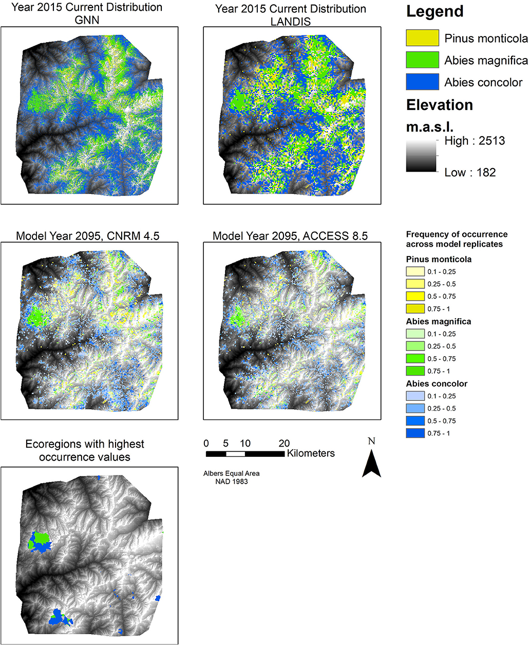
Figure 2. Current and future projected distributions of three species. Top left shows the current distribution of these species from the GNN dataset. Top right shows initial distribution in LANDIS. Middle left map shows distributions in 2095 under CNRM rcp 4.5 (a warmer and wetter projection). Middle right map shows distributions in 2095 under ACCESS rcp 8.5 (a hotter and drier projection). The middle maps are composites of the seven model replicates: they represent an average of how often a particular cell was occupied by that species. A value of one indicates that that species was present in that cell across all seven replicates. A value of >0.5 indicates that that species was present in more than half of the replicates. Bottom left map shows the climate ecoregions that were the most favorable for each species through the entire simulation duration.

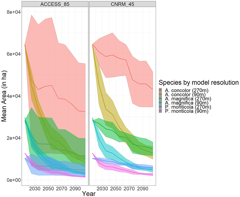
Figure 3. Mean area, in hectares, occupied by specific conifer species, under different model resolutions and different climate change projections.

We evaluated how model resolution affected species' behavior on the landscape by comparing our three metrics (Figure 4). Trends in the elevation each species occupied remained consistent across the different model resolutions and climate projections; minimum elevation increased (~50–100 m depending on species and climate) as the cohorts that occupied the lowest elevation cells were killed while mean elevation declined (~20–70 m). There were significant differences between patch sizes and the different model resolutions, the coarser resolution model resulted in much larger mean sizes (1,000 vs. 400 hectares, respectively for A. magnifica in year 2015) and maximum patch sizes (10 x 10⁴ hectares vice 6 x 10⁴ hectares for A. concolor in 2015).

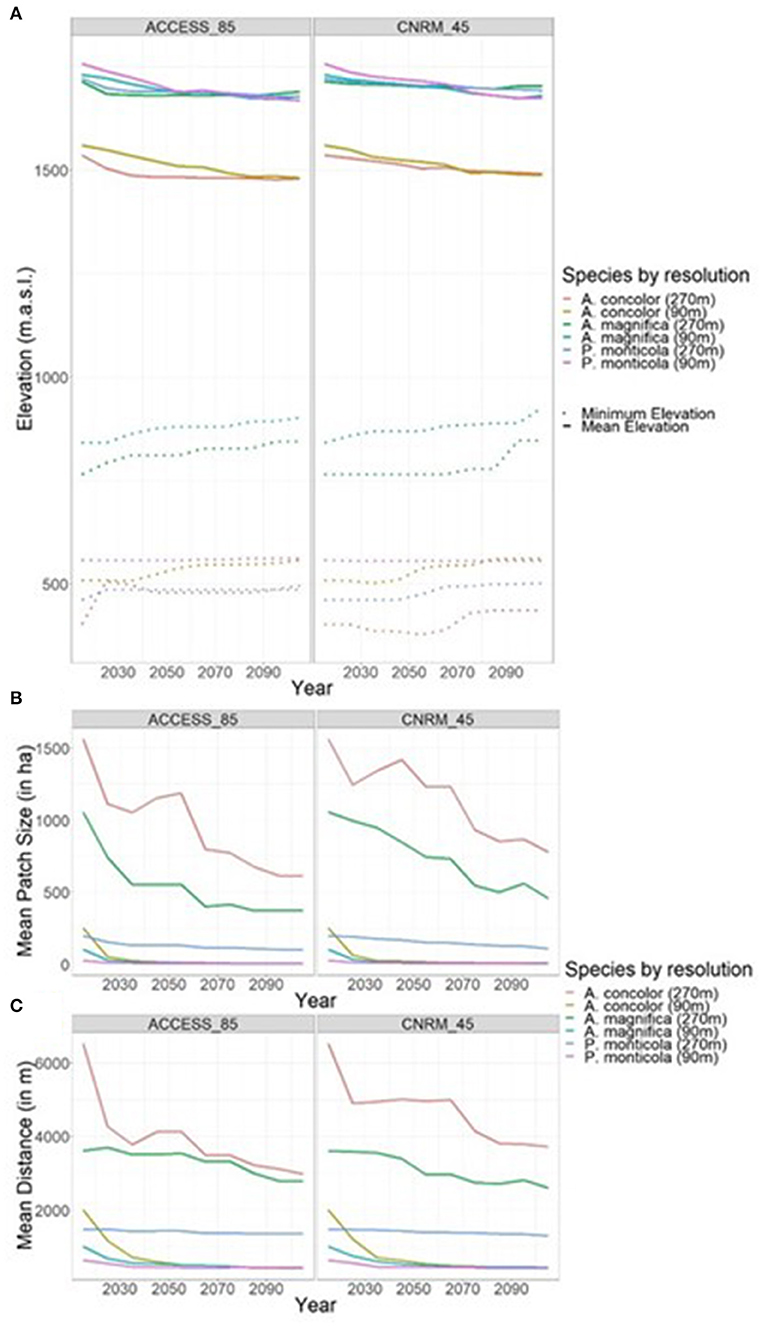
Figure 4. Patch metrics of specific conifer species, under different model resolutions and different climate change projections. (A) Mean elevation (m.a.s.l.) of species (solid line) and minimum elevation of species (dotted line). Middle: mean patch size (in hectares). (B) Mean patch size (in hectares). (C) Mean distance between patches (in meters).

Climate change significantly reduced regeneration, which in turn affected species demographics. Probability of establishment for all three species remained relatively constant under a contemporary climate but declined significantly with increased forcing (Figure S8A). By the end of the century, establishment fell to zero under the hottest projections (ACCESS RCP 8.5 and CanESM RCP 8.5). This is turn resulted in the declines of area occupied by cohorts under age 20 (Figure S8B). However, the amount of area occupied by cohorts older than 200 years increased, regardless of climate, but was tempered by the hottest climate projections which had the larger and more severe fires. This survivorship by older trees is likely overstated on the account of insect mortality, as larger trees are preferred hosts, which was not accounted for in this study (Fettig et al., 2019).

Combining all three species presence values, the 0.81 ha simulation produced a more fragmented landscape than the coarser resolution (Figure 5). The 270 m results show a higher concentration of high values in the NW quadrant of the study area. The map of differences between the results of the two different resolutions illustrates these trends: high levels of disagreement exist in that NW quadrant and along the eastern border (Figure 5).

Figure 5. (Left) Map of occupancy for the three species in year 2105 for the 90 m model, averaged across seven replicates and scaled between 0 (no species present in cell) and 1 (all species present in cell). (Middle) Map of occupancy for the three species in year 2105 for the 270 m model, averaged across nine replicates. (Right) Difference between the two (90 m map minus the 270 m map).

The model coefficient sizes and direction for relationships of species occurrence to environmental variables were similar between the two climate projections (Table 1). The majority slope of the ecoregion was a strong predictor: the coefficient was negative and significant for all species and climate projections. Increasing the percent slope of the ecoregion decreased the proportion of ecoregion occupied by each species. Precipitation had a positive relationship with the occurrence of the two fir species, though only significant for white fir, and negative for the pine; maximum temperature exhibited the same patterns. The interaction term between precipitation and temperature was negative for the firs and positive for the pine species. As a result, increasing temperature and precipitation would increase fir presence to a certain extent. The opposite is applicable to pines, where the species would be more likely to persist on colder and drier environments. The elevation coefficient was positive and significant for red fir and pines, reflecting species that are better suited for higher elevation environments. Aspect and the soil available water capacity were found to be insignificant for any species. Rho, the spatial weight term, was found to be positive and significant only for white fir. Other variables were considered for the model but were not found significant, specifically the average number of times each cell burned in each ecoregion.

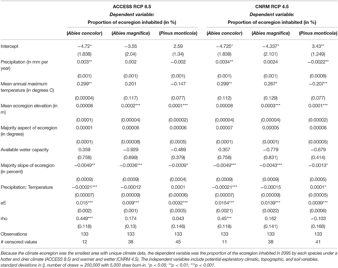
Table 1. Table of spatially autoregressive two way tobit model, mean and standard deviation of the posterior distribution for the coefficients presented, as well as respective p-values.

Discussion

Our findings are similar to a number of other studies showing widespread decline of high elevation species under climate change (Bell et al., 2014a; Harvey et al., 2016; Andrus et al., 2018; DeSiervo et al., 2018, among others). Species distribution models based on data from the Forest Inventory and Analysis National Program estimated a significant decrease in climate suitability for high elevation species, not only for current distributions but also for areas that those species could possibly move into (Bell et al., 2014a). In addition, conifer seedling establishment was found to decline after fire events due to soil moisture limitations, while another study found that that conifer establishment was strongly linked to high soil moisture and cool/wet summer conditions (Harvey et al., 2016; Andrus et al., 2018). More specifically for this landscape, in the adjacent Russian Wilderness, a decline in fir species was associated with increasing winter minimum temperatures and presence of pathogens (DeSiervo et al., 2018). Our findings are also likely overestimating species persistence given the high levels of insect mortality that occurred in 2017 as the result of a multi-year drought in California (Fettig et al., 2019).

While other studies have found instances of a species migrating up in elevation to stay within its suitable climate (Chen et al., 1999; Kelly and Goulden, 2008), our findings are less straightforward. The minimum elevation each species occupies does increase, which coincides with those findings, but with results depending on the species, the model resolution, and the climate forcing (e.g., a 93 m increase for A. concolor under ACCESS RCP 8.5 at the 270 m resolution vs. 48 at 90 m, a 41 m increase for P. monticola under CNRM RCP 4.5 at 270 vs. 2 m for the 90 m model). This result likely can be attributed to model resolution as averaged minimum starting elevations were different between resolutions. As a whole, minimum elevations changed little, indicating that certain established sites were able to persist even through climate disequilibrium. While this might point to the possibility of holdouts existing on the landscape, the issues of the directionality of climate change and whether these species are able to regenerate under increasing temperatures does not guarantee long term species persistence. Other researchers have found that young trees are more vulnerable to changes in climate (Bell et al., 2014b; Dobrowski et al., 2015), which points to an increasing likelihood of extinction debt as the species cannot reproduce itself (Kuussaari et al., 2009). While the LANDIS-II model does not ascribe different climate tolerances to different age classes, the declining probability of establishment, in effect, creates a similar demographic effect.

The expectation that climate sensitive species would move upslope in order to stay within their ideal climate was not met, as the mean elevation that these species occupied across the landscape declined slightly. A number of other researchers have found similar results (Crimmins et al., 2011; Millar et al., 2012; Serra-Diaz et al., 2014) for various other reasons (e.g., disturbance, changing water balance due to declining snowpack). However, because these species could not go any higher because they were already occupying the highest elevations, these averages were sensitive to changes at the highest elevations. But because the model does not directly simulate mortality from drought, these results are likely underestimating the upward shift in elevation of the species distributions, especially given the high mortality from the recent drought in California (Young et al., 2017).

While distance between patches was significantly different between model resolutions, the mean distance was beyond the effective seed dispersal distances for each of the species, though not beyond the potential long-distance dispersal (for the 90 m resolution model). A sensitivity test tripling dispersal distances found the same overall decline, although at a slower rate (see Figure S9). Additional testing—running the model without the fire extension (data not shown), such that there was no disturbance mortality—increased the amount of biomass for each species across the landscape but saw regeneration rates still decline due to climate change. Because the large patches are breaking into smaller patches that are close together, the mean distance between patches declines through time. As the small patches are eliminated from the landscape, it is expected that the distance between patches would start to increase again. Because these species regenerate best on mineral soil after snowmelt (Graham, 1990; Laacke, 1990a,b), there is a possible positive feedback under climate change, where the decrease in canopy cover results in reduced shade which results in increasing snow ablation (Varhola et al., 2010) which reduces the likelihood of successful regeneration. One potential consequence of isolated patches is the genetic degradation associated with the stop of gene flow, but Kramer et al. (2008). suggest that genetic degradation is less important than ecological degradation following habitat fragmentation. With the unidirectional pressure of climate change and the decline of these species, these species will likely be extirpated from the landscape before they experience the genetic declines of inbreeding.

Management Implications

The declines of high elevation species are going to be substantial under climate change; increasing temperatures and drought stress cause climate disequilibrium, regeneration will decline, microrefugia will likely be rare (there are only a handful of candidate ecoregions, Figure 2), while competition and dispersal limitations will limit the ability of the species to move across the landscape. While the situation appears dire, there is still time for managers to intervene, if they so choose. Trees are long-lived organisms, and old trees are more resistant to climate disequilibrium—the amount of area occupied by old cohorts is increasing by the end of the century (Figure S8B). However, this prompts a larger discussion about the goals of forest management. While these trees might disappear from the Klamath Range, they are also present in the Cascade Range, a continuous mountain range that might be more conducive to migration though additional research would be necessary. There will be a period of time where these areas might be unforested while Doug-fir and other conifers move up in elevation, but instead of using resources to maintain the current species distributions, efforts could be made to move lower elevation species uphill to maintain forest cover.

Assisted migration, while controversial, may become an important tool. Pedlar et al. (2012) break down assisted migration into two forms, forestry and survival assisted migration. Survival assisted migration, or translocation outside of native range, might be necessary for persistence of the endemic species of the Klamath region (e.g., Brewer spruce). Forestry assisted migration, arguably less controversial, is already happening on the landscape as industrial forestry practices selectively breed trees to be resistant to climate change without necessarily planting those trees outside of their natural range (Leech et al., 2011; Pedlar et al., 2012). While introducing southern provenances of these species would likely bring increased temperature and drought resistance, research trials to investigate many factors (e.g., successful regeneration, invasiveness) at individual and stand scales would be necessary before widespread introduction. One advantage of using a forest simulation model is that it is possible to run large scale experiments on the landscape, including testing the introduction of species from outside of the study area (Duveneck and Scheller, 2015). While modeling may not necessarily address the possibility of how invasive an introduced species might be, a main concern of assisted migration, it can address general efficacy and limitations.

Conclusion

There are multiple streams of evidence that high elevation species are at greater risk under climate change, and the results of this modeling study add to that body of evidence. These montane conifer species are expected to decline significantly by the end of the century. While model resolution mattered for how these species were distributed across the landscape, they were ultimately reliant on lower resolution climate data which likely limited the ability to find microclimates that might allow pockets of these species to persist. Nevertheless, there is still opportunity for forest managers to intervene if desired; however, there are many technical and conceptual issues that need to be addressed before moving species around as part of a large-scale management approach. Decisions about what to do need to recognize the larger landscape; these species are widely distributed across the Western US. But with so few areas where these species were able to persist, there will be a lag between these species dying off before lower elevation conifers can move up the landscape to occupy those areas. Nevertheless, assisted migration may have a role to play with Brewer spruce as a high elevation endemic species. Otherwise, with warming temperatures and no place to go, only the adults of these species will likely persist and only until disturbance removes them.

Data Availability Statement

All model inputs and parameters necessary to run the model and recreate the results are available through https://github.com/LANDIS-II-Foundation/Project-Klamath-Climate-Fire/tree/master/MMW.

Author Contributions

CM designed the experiment and analyzed the results. CM and RS equally contributed to the interpretation of the results and writing of the manuscript.

Funding

This material is based upon work supported by National Science Foundation Collaborative Research Grant #1353509 and National Science Foundation IGERT Grant #0966376. Additional computing support was provided by the Microsoft Azure for Research Award. The views expressed here are those of the authors and do not necessarily represent the views or policies of the National Science Foundation.

Conflict of Interest

The authors declare that the research was conducted in the absence of any commercial or financial relationships that could be construed as a potential conflict of interest.

Acknowledgments

Previous drafts of this manuscript were improved by assistance from Alexandra Syphard, Tom Spies, and two reviewers.

Supplementary Material

The Supplementary Material for this article can be found online at: https://www.frontiersin.org/article/10.3389/ffgc.2019.00094/full#supplementary-material.

References

Andrus, R. A., Harvey, B. J., Rodman, K. C., Hart, S. J., and Veblen, T. T. (2018). Moisture availability limits subalpine tree establishment. Ecology 99, 567–575. doi: 10.1002/ecy.2134
Beedlow, P. A., Lee, E. H., Tingey, D. T., Waschmann, R. S., and Burdick, C. A. (2013). The importance of seasonal temperature and moisture patterns on growth of Douglas-fir in western oregon, USA. Agric. For. Meteorol. 169, 174–185. doi: 10.1016/j.agrformet.2012.10.010
Bell, D. M., Bradford, J. B., and Lauenroth, W. K. (2014a). Early indicators of change: divergent climate envelopes between tree life stages imply range shifts in the western United States. Glob. Ecol. Biogeogr. 23, 168–180. doi: 10.1111/geb.12109
Bell, D. M., Bradford, J. B., and Lauenroth, W. K. (2014b). Mountain landscapes offer few opportunities for high-elevation tree species migration. Glob. Change Biol. 20, 1441–1451. doi: 10.1111/gcb.12504
Burns, R. M., and Honkala, B. H. (Eds). (1990). Silvics of North America: Volume 1. Conifers. Washington, DC: U.S. Dept. of Agriculture, Forest Service.
Chen, J., Saunders, S. C., Crow, T. R., Naiman, R. J., Brosofske, K. D., Mroz, G. D., et al. (1999). Microclimate in forest ecosystem and landscape ecology: variations in local climate can be used to monitor and compare the effects of different management regimes. Bioscience 49, 288–297. doi: 10.2307/1313612
Cheng, S. (2004). Forest Service Research Natural Areas in California. Albany, CA: Pacific Southwest Research Station; Forest Service, US Department of Agriculture.
Copenhaver-Parry, P. E., Shuman, B. N., and Tinker, D. B. (2017). Toward an improved conceptual understanding of North American tree species distributions. Ecosphere 8:e01853. doi: 10.1002/ecs2.1853
Crimmins, S. M., Dobrowski, S. Z., Greenberg, J. A., Abatzoglou, J. T., and Mynsberge, A. R. (2011). Changes in climatic water balance drive downhill shifts in plant species' optimum elevations. Science 331, 324–327. doi: 10.1126/science.1199040
DeSiervo, M. H., Jules, E. S., Bost, D. S., De Stigter, E. L., and Butz, R. J. (2018). Patterns and drivers of recent tree mortality in diverse conifer forests of the Klamath mountains, California. For. Sci. 64, 371–382. doi: 10.1093/forsci/fxx022
Dobrowski, S. Z. (2011). A climatic basis for microrefugia: the influence of terrain on climate. Glob. Change Biol. 17, 1022–1035. doi: 10.1111/j.1365-2486.2010.02263.x
Dobrowski, S. Z., Swanson, A. K., Abatzoglou, J. T., Holden, Z. A., Safford, H. D., Schwartz, M. K., et al. (2015). Forest structure and species traits mediate projected recruitment declines in western US tree species. Glob. Ecol. Biogeogr. 24, 917–927. doi: 10.1111/geb.12302
Duveneck, M. J., and Scheller, R. M. (2015). Climate-suitable planting as a strategy for maintaining forest productivity and functional diversity. Ecol. Appl. 25, 1653–1668. doi: 10.1890/14-0738.1
Fettig, C. J., Mortenson, L. A., Bulaon, B. M., and Foulk, P. B. (2019). Tree mortality following drought in the central and southern Sierra Nevada, California, US. For. Ecol. Manage. 432, 164–178. doi: 10.1016/j.foreco.2018.09.006
Franklin, J. (2010). Moving beyond static species distribution models in support of conservation biogeography. Divers. Distrib. 16, 321–330. doi: 10.1111/j.1472-4642.2010.00641.x
Graham, R. T. (1990). “Pinus monticola,” in Silvics of North America: Volume 1. Conifers, eds R. M. Burns and B. H. Honkala (Washington, DC: U.S. Dept. of Agriculture, Forest Service), 385–394.
Hannah, L., Flint, L., Syphard, A. D., Moritz, M. A., Buckley, L. B., and McCullough, I. M. (2014). Fine-grain modeling of species' response to climate change: holdouts, stepping-stones, and microrefugia. Trends Ecol. Evol. 29, 390–397. doi: 10.1016/j.tree.2014.04.006
Harvey, B. J., Donato, D. C., and Turner, M. G. (2016). High and dry: post-fire tree seedling establishment in subalpine forests decreases with post-fire drought and large stand-replacing burn patches. Glob. Ecol. Biogeogr. 25, 655–669. doi: 10.1111/geb.12443
Hurteau, M. D., Robards, T. A., Stevens, D., Saah, D., North, M., and Koch, G. W. (2014). Modeling climate and fuel reduction impacts on mixed-conifer forest carbon stocks in the Sierra Nevada, California. For. Ecol. Manage. 315, 30–42. doi: 10.1016/j.foreco.2013.12.012
Kelly, A. E., and Goulden, M. L. (2008). Rapid shifts in plant distribution with recent climate change. Proc. Natl. Acad. Sci. U.S.A. 105, 11823–11826. doi: 10.1073/pnas.0802891105
Keppel, G., Van Niel, K. P., Wardell-Johnson, G. W., Yates, C. J., Byrne, M., Mucina, L., et al. (2012). Refugia: identifying and understanding safe havens for biodiversity under climate change. Glob. Ecol. Biogeogr. 21, 393–404. doi: 10.1111/j.1466-8238.2011.00686.x
Kim, J. B., Kerns, B. K., Drapek, R. J., Pitts, G. S., and Halofsky, J. E. (2018). Simulating vegetation response to climate change in the Blue Mountains with MC2 dynamic global vegetation model. Clim. Serv. 10, 20–32. doi: 10.1016/j.cliser.2018.04.001
Kramer, A. T., Ison, J. L., Ashley, M. V., and Howe, H. F. (2008). The paradox of forest fragmentation genetics. Conserv. Biol. 22, 878–885. doi: 10.1111/j.1523-1739.2008.00944.x
Kuussaari, M., Bommarco, R., Heikkinen, R. K., Helm, A., Krauss, J., Lindborg, R., et al. (2009). Extinction debt: a challenge for biodiversity conservation. Trends Ecol. Evol. 24, 564–571. doi: 10.1016/j.tree.2009.04.011
Laacke, R. J. (1990a). “Abies concolor,” in Silvics of North America, Volume 1. Conifers, eds R. M. Burns and B. H. Honkala (Washington, DC: U.S. Dept. of Agriculture, Forest Service), 36–46.
Laacke, R. J. (1990b). “Abies magnifica,” in Silvics of North America: Volume 1. Conifers, eds R. M. Burns and B. H. Honkala (Washington, DC: U.S. Dept. of Agriculture, Forest Service), 71–79.
Lee, E. H., Beedlow, P. A., Waschmann, R. S., Tingey, D. T., Wickham, C., Cline, S., et al. (2016). Douglas-fir displays a range of growth responses to temperature, water, and swiss needle cast in western Oregon, USA. Agric. For. Meteorol. 221, 176–188. doi: 10.1016/j.agrformet.2016.02.009
Leech, S. M., Almuedo, P. L., and O'Neill, G. (2011). Assisted migration: adapting forest management to a changing climate. J. Ecosyst. Manage. 12, 1–17. Available online at: https://jem-online.org/forrex/index.php/jem/article/view/91/98 (accessed January 01, 2020).
Lenoir, J., Gégout, J., Marquet, P. A., De Ruffray, P., and Brisse, H. (2008). A significant upward shift in plant species optimum elevation during the 20th century. Science 320, 1768–1771. doi: 10.1126/science.1156831
Levin, S. A. (1992). The problem of pattern and scale in ecology: the Robert H. MacArthur award lecture. Ecology 73, 1943–1967. doi: 10.2307/1941447
Liang, S., Hurteau, M. D., and Westerling, A. L. (2017). Response of Sierra Nevada forests to projected climate–wildfire interactions. Glob. Change Biol. 23, 2016–2030. doi: 10.1111/gcb.13544
Lucash, M. S., and Scheller, R. M. (2015). LANDIS-II Climate Library v1. 0 User Guide. Available online at: https://drive.google.com/file/d/0B6eUM6Se6MFBZ2FiWmx2b3g2RXM/view (accessed January 01, 2020).
Malanson, G. P., Butler, D. R., Fagre, D. B., Walsh, S. J., Tomback, D. F., Daniels, L. D., et al. (2007). Alpine treeline of western North America: linking organism-to-landscape dynamics. Phys. Geogr. 28, 378–396. doi: 10.2747/0272-3646.28.5.378
Maurer, E. P., Wood, A. W., Adam, J. C., Lettenmaier, D. P., and Nijssen, B. (2002). A long-term hydrologically based dataset of land surface fluxes and states for the conterminous united states. J. Clim. 15, 3237–3251. doi: 10.1175/JCLI-D-12-00508.1
Millar, C. I., Westfall, R. D., Delany, D. L., Bokach, M. J., Flint, A. L., and Flint, L. E. (2012). Forest mortality in high-elevation whitebark pine (Pinus albicaulis) forests of eastern California, USA; influence of environmental context, bark beetles, climatic water deficit, and warming. Can. J. For. Res. 42, 749–765. doi: 10.1139/x2012-031
Ohmann, J. L., Gregory, M. J., Henderson, E. B., and Roberts, H. M. (2011). Mapping gradients of community composition with nearest-neighbour imputation: extending plot data for landscape analysis. J. Veget. Sci. 22, 660–676. doi: 10.1111/j.1654-1103.2010.01244.x
Parker, A. J. (1982). The topographic relative moisture index: an approach to soil-moisture assessment in mountain terrain. Phys. Geogr. 3, 160–168. doi: 10.1080/02723646.1982.10642224
Pedlar, J. H., McKenney, D. W., Aubin, I., Beardmore, T., Beaulieu, J., Iverson, L., et al. (2012). Placing forestry in the assisted migration debate. Bioscience 62, 835–842. doi: 10.1525/bio.2012.62.9.10
Scheller, R. M., Domingo, J. B., Sturtevant, B. R., Williams, J. S., Rudy, A., Gustafson, E. J., et al. (2007). Design, development, and application of LANDIS-II, a spatial landscape simulation model with flexible temporal and spatial resolution. Ecol. Model. 201, 409–419. doi: 10.1016/j.ecolmodel.2006.10.009
Scheller, R. M., Hua, D., Bolstad, P. V., Birdsey, R. A., and Mladenoff, D. J. (2011). The effects of forest harvest intensity in combination with wind disturbance on carbon dynamics in lake states mesic forests. Ecol. Model. 222, 144–153. doi: 10.1016/j.ecolmodel.2010.09.009
Serra-Diaz, J. M., Franklin, J., Ninyerola, M., Davis, F. W., Syphard, A. D., Regan, H. M., et al. (2014). Bioclimatic velocity: the pace of species exposure to climate change. Divers. Distribut. 20, 169–180. doi: 10.1111/ddi.12131
Serra-Diaz, J. M., Maxwell, C., Lucash, M. S., Scheller, R. M., Laflower, D. M., Miller, A. D., et al. (2018). Disequilibrium of fire-prone forests sets the stage for a rapid decline in conifer dominance during the 21st century. Sci. Rep. 8, 1–12. doi: 10.1038/s41598-018-24642-2
Smithers, B. V., North, M. P., Millar, C. I., and Latimer, A. M. (2018). Leap frog in slow motion: divergent responses of tree species and life stages to climatic warming in Great Basin subalpine forests. Glob. Change Biol. 24, e442–e457. doi: 10.1111/gcb.13881
Soil Survey Staff Natural Resources Conservation Service, United States Department of Agriculture. (2019). Web Soil Survey. Available online at: https://websoilsurvey.nrcs.usda.gov/ (accessed October 2, 2018).
Svenning, J., Eiserhardt, W. L., Normand, S., Ordonez, A., and Sandel, B. (2015). The influence of paleoclimate on present-day patterns in biodiversity and ecosystems. Annu. Rev. Ecol. Evol. Syst. 46, 551–572. doi: 10.1146/annurev-ecolsys-112414-054314
Svenning, J., and Sandel, B. (2013). Disequilibrium vegetation dynamics under future climate change. Am. J. Bot. 100, 1266–1286. doi: 10.3732/ajb.1200469
Taylor, A. H., and Skinner, C. N. (2003). Spatial patterns and controls on historical fire regimes and forest structure in the Klamath mountains. Ecol. Appl. 13, 704–719. doi: 10.1890/1051-0761(2003)013[0704:SPACOH]2.0.CO;2
Thompson, J. R., and Spies, T. A. (2009). Vegetation and weather explain variation in crown damage within a large mixed-severity wildfire. For. Ecol. Manage. 258, 1684–1694. doi: 10.1016/j.foreco.2009.07.031
Thompson, J. R., and Spies, T. A. (2010). Factors associated with crown damage following recurring mixed-severity wildfires and post-fire management in southwestern Oregon. Landsc. Ecol. 25, 775–789. doi: 10.1007/s10980-010-9456-3
Varhola, A., Coops, N. C., Weiler, M., and Moore, R. D. (2010). Forest canopy effects on snow accumulation and ablation: an integrative review of empirical results. J. Hydrol. 392, 219–233. doi: 10.1016/j.jhydrol.2010.08.009
Ward, B. C., Scheller, R. M., and Mladenoff, D. J. (2004). Technical Report: LANDIS-II Double Exponential Seed Dispersal Algorithm. University of Wisconsin, Madison, WI, 5. Available online at: https://docs.google.com/file/d/0B6eUM6Se6MFBbFc4TUpTMGx5a0k/edit?usp=sharing (accessed January 01, 2020).
Westerling, A. L., Hidalgo, H. G., Cayan, D. R., and Swetnam, T. W. (2006). Warming and earlier spring increase western US forest wildfire activity. Science 313, 940–943. doi: 10.1126/science.1128834
Whittaker, R. H. (1960). Vegetation of the Siskiyou mountains, Oregon and California. Ecol. Monogr. 30, 279–338. doi: 10.2307/1943563
Wilson, B. T., Woodall, C. W., and Griffith, D. M. (2013). Imputing forest carbon stock estimates from inventory plots to a nationally continuous coverage. Carbon Balance Manage. 8:1. doi: 10.1186/1750-0680-8-1
Young, D. J., Stevens, J. T., Earles, J. M., Moore, J. N., Ellis, A., Jirka, A. L., et al. (2017). Long-term climate and competition explain forest mortality patterns under extreme drought. Ecol. Lett. 20, 78–86. doi: 10.1111/ele.12711
Zouhar, K. (2001). Fire effects information system (FEIS) – Abies concolor. Available online at: https://www.fs.fed.us/database/feis/plants/tree/abicon/all.html (accessed January 01, 2020).
Keywords: climate change, simulation modeling, species distributions, Klamath Mountains, LANDIS-II
Citation: Maxwell CJ and Scheller RM (2020) Identifying Habitat Holdouts for High Elevation Tree Species Under Climate Change. Front. For. Glob. Change 2:94. doi: 10.3389/ffgc.2019.00094
Received: 20 September 2019; Accepted: 24 December 2019;
Published: 21 January 2020.
Edited by:
Brian J. Palik, Northern Research Station, Forest Service (USDA), United StatesReviewed by:
Toni Lyn Morelli, United States Geological Survey (USGS), United StatesMaxime Cailleret, National Research Institute of Science and Technology for Environment and Agriculture (IRSTEA), France
Copyright © 2020 Maxwell and Scheller. This is an open-access article distributed under the terms of the Creative Commons Attribution License (CC BY). The use, distribution or reproduction in other forums is permitted, provided the original author(s) and the copyright owner(s) are credited and that the original publication in this journal is cited, in accordance with accepted academic practice. No use, distribution or reproduction is permitted which does not comply with these terms.
*Correspondence: Charles J. Maxwell, cjmaxwe3@ncsu.edu