A Monte Carlo Method for Quantifying Uncertainties in the Official Greenhouse Gas Emission Factors Database of Costa Rica

Introduction

The latest National Surveys on Climate Change (UNDP and UCR, 2014; MINAE and UNDP, 2021) revealed that most of the Costa Rican population is aware that there are risks associated with climate change that can already be perceived and they agree to take action to fight against this global enemy. Accordingly, the government of Costa Rica has launched national policies and programs that seek to decarbonize its economy (Government of Costa Rica, 2019) and adapt to the climate change consequences (Government of Costa Rica, 2018), including the National Carbon Neutrality Program (PPCN, by its Spanish acronym) (DCC and PMR, 2020). Thanks to these efforts, Costa Rica was recognized with the Champions of Earth Policy Leadership Award (UNEP, 2019), but many challenges still remain.

With the publication of the latest version of ISO 14064-1 (2018), the PPCN included measurement uncertainty as a mandatory requirement for the reporting of greenhouse gas (GHG) inventories as an essential parameter to have precise and reliable data for the correct quantification of emissions and removals (DCC and PMR, 2020). Measurement uncertainty, formally defined as the doubt about the true value of a quantity that remains after making its measurement or estimation, is the best quality parameter of any measurement or estimation and reflects the impossibility of knowing exactly its value (JCGM, 2008a). Among the accepted methodologies for estimating uncertainty, the law of propagation of uncertainty included in the Guide to the Expression of Uncertainty in Measurement (GUM) and the Monte Carlo simulation method included in the Supplement 1 of the GUM (GUM-S1) stand out. These methodologies are based on modeling an output quantity $y$ as a known function of several input quantities $x_i$ and handles the uncertainties associated with the input quantities by modeling them as random variables with defined probability distributions. These approaches use the on-hand information about the input quantities to produce an approximate evaluation of the uncertainty of the output quantity through a first-order Taylor series expansion or a propagation of probability distributions using simulation techniques (JCGM, 2008a; JCGM, 2008b).

In the context of GHG inventories, uncertainty estimation has been pointed as a key component to increase confidence in the reported results and help decision makers to better target areas for implementing mitigation strategies and policy development (El-Fadel et al., 2001; EPA, 2002; IIASA, 2007; Jonas et al., 2010a; Jonas et al., 2010b; Hergoualch et al., 2021). Several studies have been developed regarding this topic, including EPA (1996), Bharvirkar (1999), Frey (2007), Ritter et al. (2010), Pouliot et al. (2012), Milne et al. (2015), Quilcaille et al. (2018), and Solazzo et al. (2021), among others. With the publication of IPCC Guidelines for National Greenhouse Gas Inventories (IPCC, 2000; IPCC, 2006a; IPCC, 2019a), it was possible to establish a globally approved framework to estimate uncertainties in this field, based on both methodologies described in the GUM and GUM-S1. It has been pointed out that the first method may be easier to implement and suitable for calculating uncertainties from uncorrelated, normally distributed individual input estimates with variation ranges below ±30%, but it can lead to significant uncertainty underestimations when these restrictions are breached (Fauser et al., 2011; Wójcik-Gront and Gront, 2014). The Monte Carlo simulation method allows for different probability distribution functions, parameter correlations, complex models, and large uncertainties, making it more attractive for a wider range of cases. Applications of the Monte Carlo uncertainty estimation method in the field of GHG emission includes Monni et al. (2004), Ramírez et al. (2008), Fauser et al. (2011), Silva et al. (2011), Wójcik-Gront and Gront (2014), Caldwallader and VanBriesen (2017), and Cho et al. (2018), among others.

In Costa Rica, additional technical guidelines were developed to aid the implementation of uncertainty estimation in GHG inventories (DCC and LCM, 2020). Also, a study by Molina-Castro and Calderón-Jiménez (2021) served to complement and update the official database of Costa Rican emission factors (IMN, 2021), providing uncertainty values for the emission factors of the fuel sector and methodological guidance to approach uncertainty estimation of emission factors using asymmetric probability distributions. However, technical gaps still remain for an optimal implementation of uncertainty estimation in the GHG inventories of Costa Rica, including a lack of information regarding uncertainties of the national emission factors for the agricultural, waste treatment, livestock, and industrial sectors from the Costa Rican official database. Although studies carried out in other countries can be found to estimate emission factors and their uncertainties in the sectors mentioned above (for example Milne et al. (2014) and Monni et al. (2007) for agriculture, Zheng et al. (2004) for croplands, Caldwallader and VanBriesen (2017) for wastewater, Basset-Mens et al. (2009) for livestock, among others), no related works have been carried out in Costa Rica. These gaps are becoming serious limitations that prevent the reporting of complete, transparent, and reliable emission results that meet the nationally established requirements, urging the development of national-specific studies that complete the missing information.

This article sought to fill the gap of uncertainty information that the official database of Costa Rican emission factors currently has, providing values for the missing uncertainties of emission factors through the collection of information and application of the Monte Carlo simulation method where needed. It should be remembered that emission factors are key elements for indirect quantification of emissions, where emissions ($E$) are not measured directly as an amount of gas released into the atmosphere but estimated from other data values associated with the activity that cause the emission ($d$) and emission factors ($f$) that relate these data to the amount of gas emitted, as shown in Eq. 1.

Therefore, according to the GUM uncertainty estimation principles mentioned previously, emission factor uncertainties are necessary for the estimation of the emission uncertainty. As a consequence of the process followed to achieve the proposed objective, this study also includes suggested updates for some of the emission factors considered. It is expected that this study, together with the one previously published by Molina-Castro and Calderón-Jiménez (2021), will ease compliance with the requirements for reporting GHG emission results and will serve as a guide for uncertainty estimation and interpretation in GHG inventories in Costa Rica and other countries around the world.

Methods

Emission Factors Selection

According to the last official database published by the National Meteorological Institute of Costa Rica (IMN, by its Spanish acronym), emission factors from livestock enteric fermentation, manure management, waste treatments, most croplands and grasslands, and non-energy use of lubricants are missing uncertainty information (IMN, 2021). These factors corresponded to the initial list within the scope of the present study. However, after holding meetings with IMN experts in the field, the emission factors associated with croplands, grasslands, and enteric fermentation from cattle (including calves) were excluded since there are national unpublished studies that include uncertainty estimates for their values. It is expected that future publications of the official database will include these uncertainties. Thus, the emission factors selected for this study and their current values are shown in Table 1.

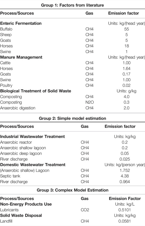
TABLE 1. Emission factors included in this study with their current values taken from the official database of emission factors of Costa Rica (IMN, 2021), classified according to their estimation methods.

Emission Factors Classification

As shown in Table 1, the emission factors included in the scope of this study were classified into three groups according to their estimation methods and their information sources. This is done because the subsequent methodological strategies used to estimate their uncertainties depend on the way the emission factors are obtained. The details of each group are shown below. For reproducibility purposes, the values, confidence intervals, and their source for all the input quantities mentioned below can be consulted in Supplementary Tables S1–S3 of the supplementary material.

Group 1: Factors From Literature

This group included emission factors with values taken directly from the literature, specifically from IPCC Guidelines (IPCC, 2006d; IPCC, 2006f; IPCC, 2019b). These factors correspond to the most basic level of emission estimation proposed by the IPCC (Tier 1) and can be used when there is no national information available. An expected variation interval with 95% confidence for these factors can usually be found within the literature. Emission factors associated with livestock enteric fermentation (other than cattle), manure management, and biological treatment of solid wastes (composting and anaerobic digestion) were included in this group.

Group 2: Simple Model Estimation

This group included emission factors (output quantities) with values estimated from simple multiplicative models with no more than three variables with uncertainty (input quantities). These factors correspond to a higher level of emission estimation proposed by the IPCC (Tier 2 or 3). For this group, the mathematical models and the values of their inputs were taken from IPCC Guidelines (IPCC, 2006g; IPCC, 2019d). An expected variation interval with 95% confidence for the input variables can also be found in these guidelines. Emission factors associated with wastewater treatments and discharge were included in this group.

For industrial wastewater treatments (anaerobic reactor and anaerobic lagoon) and river discharge, the model used to estimate their emission factors ($f$) is shown in Eq. 2. The input quantities $B_o$ and $MCF$ correspond to the maximum CH₄ producing capacity and the Methane Correction Factor (a fraction between 0 and 1), respectively (IPCC, 2006g; IPCC, 2019d).

It should be mentioned that no variation intervals were found for $MCF$ in industrial wastewater. Therefore, expert judgment was used to fill in this missing information, following the IPCC recommendations for this case (IPCC, 2006g). The criteria of three national technical experts in wastewater treatment and its emissions were used.

For domestic wastewater treatments (septic tank and anaerobic lagoon) and river discharge, the model used to estimate their emission factors ($f$) is shown in Eq. 3. The additional input quantity $BOD$ corresponds to the Biochemical Oxygen Demand (BOD) per capita estimated for the specific country or region under analysis (IPCC, 2019d).

The variable $I$ is a correction factor for additional industrial BOD discharged into sewers. For this study, $I$ was not considered an input quantity but a constant (no uncertainty) equal to 1, as suggested by IPCC Guidelines for uncollected systems (IPCC, 2019d).

Group 3: Complex Model Estimation

This group included emission factors (output quantities) with values estimated from complex models including both multiplications and additions and considering more than three variables with uncertainty (input quantities). These factors correspond to a higher level of emission estimation proposed by the IPCC (Tier 2 or 3). For this group, as detailed below, the mathematical models and the values of their inputs were taken from IPCC Guidelines and other references, including measurement standards, databases, and national studies in the subject. Expected variation intervals with 95% or 100% confidence or raw data for the input variables were also found in these references. Emission factors associated with solid waste treatment by landfill and non-energy use of lubricants were included in this group.

For non-energy use of lubricants, the model used to estimate its emission factor ($f$) is shown in Eq. 4. The input quantities $A{W}_C$ and $A{W}_O$ correspond to the atomic weights of carbon and oxygen with values taken from CIAWW (2020). The quantities $ODU$, $CC$, and $NCV$ correspond to the default Oxidized During Use factor, Carbon Content, and Net Calorific Value for lubricants taken from IPCC Guidelines (IPCC, 2000c; IPCC, 2006b). The quantity ${\rho }_{r lub}$ is the mean relative density of lubricants used in Costa Rica obtained by Morales (2016), recommended by IMN and DCC experts and considered as a state-of-the-art in the subject. Finally, the quantity ${\rho }_{H2O}$ corresponds to the density of water at 15°C, reference temperature for commercial lubricants characterization, taken from ASTM D4052 standard (ASTM, 2019).

For solid waste treatment by landfill, the model used to estimate its emission factor ($f$) is shown in Eq. 5. The additional input quantity $A{W}_H$ corresponds to the atomic weight of hydrogen with value also taken from CIAWW (2020). Similar to Eqs 2, 3, the input quantity $MCF$ is a Methane Correction Factor. The sum within the parenthesis corresponds to the Degradable Organic Carbon (DOC) in the bulk waste based on its composition. It is estimated from an average of each fraction of DOC in the different types of waste ($DO{C}_i$) weighted by its mass fraction in the bulk waste ($W_i$). $DO{C}_i$ values were taken from IPCC (2006e), while $W_i$ values were defined from a national study carried out in 2002 (FEDEMUR, 2002). Finally, the quantities $DO{C}_f$ and $F$ correspond to the default fraction of DOC which decomposes in the landfill and the default fraction of CH₄ in generated landfill gas, respectively (IPCC, 2019c).

Uncertainty Estimation Methodologies

Probability Distribution Selection and Fitting

As mentioned above, uncertainty estimation processes based on GUM methodologies (JCGM, 2008a; JCGM, 2008b) require probability distributions to be defined and fitted to the input quantities. For the present study, all input quantities correspond to continuous variables, so only continuous probability distributions were considered. Based on their previous applications in the field (IPCC, 2006a; DCC and LCM, 2020; Molina-Castro and Calderón-Jiménez, 2021), the following distributions were selected: the normal distribution, the uniform distribution, the (Student’s) t-distribution, the logarithmic normal distribution, and the (asymmetric) triangular distribution. A description of each distribution and its fitting is shown below. The distribution fitted to each input quantity can be consulted in Supplementary Tables S1–S3 of the supplementary material. An example of these distributions is shown in Figure 1.

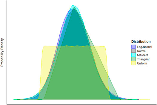
FIGURE 1. Comparison example of the probability distributions considered in the present study, fitted to a common case scenario.

Normal distribution (Laplace-Gauss distribution): The normal distribution corresponds to the probability distribution of a continuous random variable X whose density function $g_X$ is shown in Eq. 6.

The distribution parameters correspond to μ (mathematical expectation or mean) and σ (standard deviation), while $\xi$ corresponds to the variable describing the possible values of the random variable X. The normal distribution is used when the quantity values result from the additive effect of several random causes, each of which has a relatively small importance (JCGM, 2008a). It is usually recommended for the expression of expanded uncertainties in metrology and when the variation interval of the quantity is small and symmetrical to the mean (IPCC, 2006a; JCGM, 2008b). This distribution was fitted to all the symmetric input quantities taken from the IPCC guidelines and ASTM standards, whose variation intervals are or can be expressed in the form of ± U. The μ parameter was estimated with the input quantity value and the σ parameter was estimated following Eq. 7. According to the recommendations of the IPCC guidelines, a coverage factor k = 2 was considered for all cases under the assumption that the variation intervals ± U correspond to 95% confidence intervals (IPCC, 2006a).

Uniform distribution: The uniform distribution corresponds to the probability distribution of a continuous random variable X whose density function $g_X$ is shown in Eq. 8.

The distribution parameters correspond to b and a, the upper and lower bounds of the possible values, respectively. Similar to previous equations, $\xi$ is the variable describing the possible values of X. The uniform distribution is widely used when the only information available about the quantity is a lower limit and an upper limit (JCGM, 2008b; DCC and LCM, 2020). This distribution was fitted to all the atomic weights taken from CIAWW (2020) as suggested by Possolo et al. (2018). (Student’s) t-distribution: The t-distribution corresponds to the probability distribution of a continuous random variable X whose density function $g_X$ is shown in Eq. 9.

The only distribution parameter corresponds to $\upsilon$ (degrees of freedom, $\upsilon$ > 0), while Γ is the gamma function and $\xi$ is the variable describing the possible values of X. The t-distribution is used in cases similar to the normal distribution, but with finite degrees of freedom (JCGM, 2008a). It is usually recommended for the expression of expanded uncertainties in metrology and in the presence of series of replicate values representing the same quantity (JCGM, 2008b). This distribution was fitted to the density mean value of lubricants taken from Morales (2016) with 20 degrees of freedom. A normal distribution could also have been fitted for this case, but the t-distribution was preferred because it specifically included the degrees of freedom.

Logarithmic normal (log-normal) distribution: The log-normal distribution corresponds to the probability distribution of a continuous random variable X whose natural logarithm results in a normal distribution. Its density function $g_X$ is shown in Eq. 10.

The distribution parameters correspond to μ and σ, which are the mean and standard deviation of the logarithm of the normally distributed variable, respectively. Similar to previous equations, $\xi$ is the variable describing the possible values of X. The log-normal distribution may be appropriate when the variation interval for a non-negative variable is large and known to be positively skewed (IPCC, 2006a). It is also used to model the multiplication product between many uncertain quantities, which asymptotically approaches to log-normality (JCGM, 2008b). This distribution was fitted to inputs taken from IPCC guidelines with asymmetric variation intervals whose limits are far from physical boundary values like 0. Other asymmetric distributions such as the generalized extreme value distribution (Johnson et al., 1995) or the skew-normal distribution (Azzalini and Capitanio, 2014) could have been fitted for these cases, but the log-normal distribution was preferred because of its widespread use in the subject. The fitting process followed the methodology described by Molina-Castro and Calderón-Jiménez (2021).

(Asymmetric) triangular distribution: The triangular distribution corresponds to the probability distribution of a continuous random variable X whose density function $g_X$ is shown in Eq. 11.

The distribution parameters correspond to b, a, and c, the upper and lower bounds of the possible values and its most probable value (height of the triangle), respectively. Similar to previous equations, $\xi$ is the variable describing the possible values of X. When (b–c) ≠ (c–a), the triangular distribution becomes asymmetric. The triangular distribution is widely used when the only information available about the quantity is a lower limit, an upper limit, and a preferred or most probable value (JCGM, 2008b; DCC and LCM, 2020). This distribution was fitted to inputs taken from IPCC guidelines with asymmetric variation intervals whose limits are close to physical boundary values like 0 or 1. A PERT-beta distribution (Mcbride and Mcclelland, 1967) or trimmed variants of other asymmetric distributions could have been fitted for these cases, but the asymmetric triangular distribution was preferred for its ease of understanding and its simple calculations. The fitting process followed similar methodologies as described by Molina-Castro and Calderón-Jiménez (2021) and Molina-Castro (2022), solving multiple equations systems derived geometrically from the area of the triangle (Petty and Dye, 2013).

Monte Carlo Simulation Method

The propagation of probability distributions corresponds to a key step to achieve a correct evaluation of the measurement uncertainty of an output quantity Y defined as a known function $f$ of several input quantities X_i (JCGM, 2008b; Possolo and Iyer, 2017). By defining and fitting a probability density functions $g_{Xi}$ for each of the input quantities X_i, the probability density function $g_Y$ of the output quantity Y can be propagated by solving Eq. 12.

The function $\delta (\cdot )$ denotes the Dirac delta function, while $\eta$ and ${\xi }_i$ correspond to the variables describing the possible values of the output quantity Y and random variables X_i, respectively. The Monte Carlo simulation method provides a general numerical approximation to obtain a representation of the probability density function $g_Y\left(\eta \right)$. To do this, a large number of repeated random samples (simulations) are taken from the probability density functions $g_{Xi}\left({\xi }_i\right)$ and the output of the known function $f$ is estimated each time. The set of all output values obtained this way represents the approximate distribution of Y. Finally, using a simple statistical analysis, properties of the variable Y such as its mean, standard deviation, and intervals between percentiles of interest can be estimated from the simulated data (JCGM, 2008b; Crowder et al., 2020.). The complete process is illustrated in Figure 2.

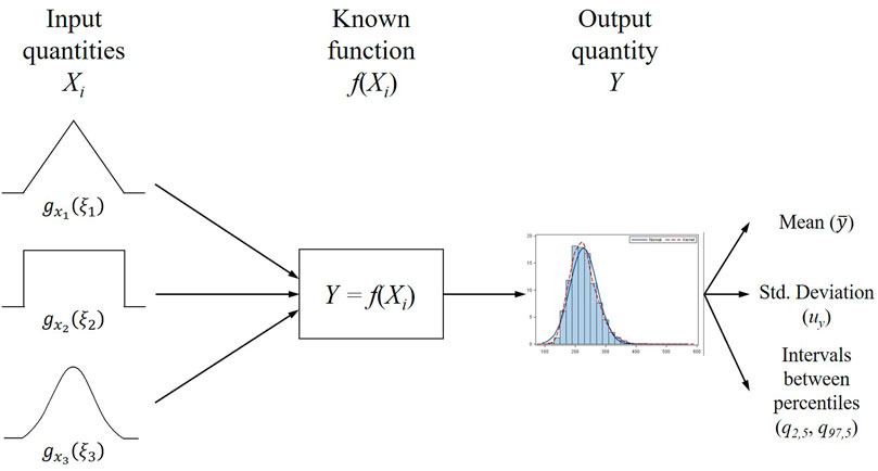
FIGURE 2. Schematic representation of the process followed to obtain a general numerical approximation of the output quantity distribution with the Monte Carlo simulation method.

The process described above was applied for all emission factors within the scope of this study. For the emission factors included in group 1, the simulation processes were carried out directly on the fitted distributions. For the emission factors included in groups 2 and 3, the simulation processes were carried out considering Eqs 2–5 for the propagation of distributions. Simulations of size 1,000 000 were used. Finally, for each set of data generated for the emission factors, its mean, standard deviation, and the interval between its 2.5% and 97.5% percentiles were estimated, corresponding to the estimated value of the emission factor, its standard uncertainty u, and its 95% confidence interval, respectively.

Data Processing

For all the calculations, statistical evaluation, and simulations, the free environment for statistical computing R version 4.1.2 (R Core Team, 2021a) was used. The R-code included sections already generated and openly provided by Possolo et al. (2019) and Molina-Castro and Calderón-Jiménez (2021). For simulations and fitting of probability distributions, computational facilities provided by R-packages triangle (Carnell, 2019), base (R Core Team, 2021b), and stats (R Core Team, 2021c) were also used.

Results and Discussion

Table 2 shows the complete results obtained from the simulations processes used for each emission factor considered. The results correspond to the estimated value of the emission factor, its standard uncertainty u, and the limits of its 95% confidence interval calculated from the simulated data population for each emission factor. All estimated standard uncertainties and limits of 95% confidence intervals are reported as absolute values. However, due to their widespread use in the GHG sector, the corresponding relative standard uncertainties and interval limits are shown in Supplementary Table S4 of the supplementary material.

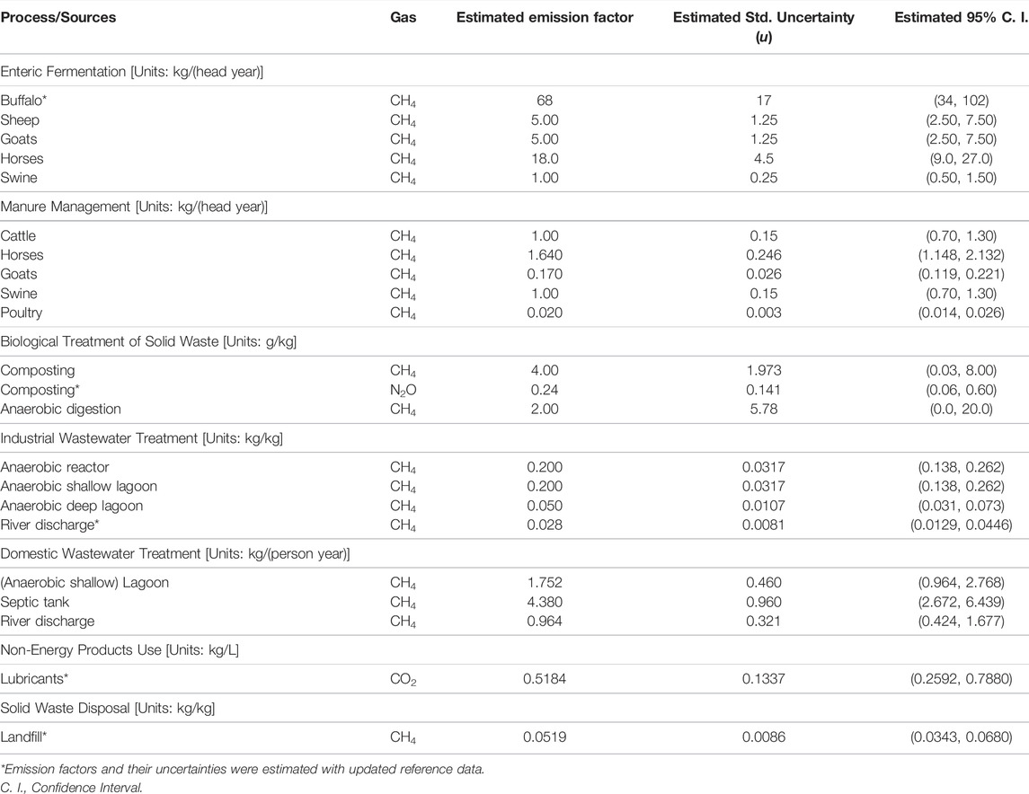
TABLE 2. Estimated values, absolute standard uncertainties, and 95% absolute confidence intervals for the emission factors using the Monte Carlo simulation method. Updated values are suggested for emission factors marked with an asterisk (*).

When comparing the values of the official emission factors shown in Table 1 with the estimated values shown in Table 2, differences are obtained for buffalo enteric fermentation, composting of solid waste (N₂O), river discharge of industrial wastewater, non-energy use of lubricants, and solid waste disposal in landfills. The reason for these differences is due to the use of updated information from the latest 2019 versions of the IPCC guidelines or other references in the present study, while the official values are based on outdated values included in the 2006 or earlier versions of these guidelines. The specific variables or input quantities updated this way are specified in Supplementary Tables S1–S3 of the supplementary material. For this reason, users and those responsible for the official list of emission factors of Costa Rica are suggested to update the emission factors according to the latest versions of the references used. The information included in Table 2 can be used for this purpose.

In this same context, it should be noted that 2019 IPCC guidelines (IPCC, 2019b) established a new methodology to estimate emissions from livestock manure management instead of the default use of recommended emission factors (Tier 1 method from IPCC, 2006d). Therefore, it is also suggested to those responsible for the official list of emission factors of Costa Rica to consider updating the values for these sources consistently with the new methodologies indicated by the updated references and evaluate their corresponding uncertainty estimations. This update could not be carried out in the present study due to the lack of data required to apply the new methodologies (IPCC, 2019b). Additionally, an update in the data used to estimate the emission factor associated with landfills is suggested. As evidenced in this study, the current official factor continues to use values of mass fractions in the bulk waste from a study conducted 20 years ago (FEDEMUR, 2002). Since then, several municipal waste composition studies have been developed in Costa Rica, including Campos-Rodríguez and Soto-Córdoba (2014), Herrera-Murillo et al. (2016), and Soto-Córdoba and González-Buitrago (2019), among others. Results from these and other studies could be used to estimate more accurate mass compositions of the bulk waste and improve the national emission factor.

The uncertainties included in Table 2 for each of the emission factors are highly relevant considering that an estimate “is complete only when accompanied by a statement of the uncertainty of that estimate” (JCGM, 2008a). Therefore, with the standard uncertainties and confidence intervals shown in Table 2, now it can be considered that these emission factors are complete estimates, useful for users of this official list who seek to estimate the uncertainty associated with their emission inventories.

It is important to note that the limits of the 95% confidence interval are usually used for expressing uncertainty in a condensed way known as expanded uncertainty ($U$) in metrology, specifically when the variation interval is symmetric to the value of the emission factor and the interval can be expressed as $f\pm U$. For asymmetric intervals, the reported limits are maintained due to their capacity to clearly express the magnitude of the variability associated with emission factors, even though they cannot be expressed in the condensed notation (IPCC, 2019a). In Supplementary Table S4 of the supplementary material, where expanded uncertainties $U$ can be easily identified, symmetrical cases in which the $\pm U$ notation could be applied include emission factors from livestock enteric fermentation ($f\pm$ 50%), manure management ($f\pm$ 30%), and industrial wastewater treatment with anaerobic reactors and shallow lagoons ($f\pm$ 31%).

It should be remembered that the standard uncertainties shown in Table 2 must be interpreted as standard deviations associated with the emission factors since the latter are considered random variables. For this reason, these uncertainties are of special interest for users since they can be combined with uncertainties of other variables (JCGM, 2008a; JCGM, 2008b). This is the case for the indirect quantification of emissions, which combines emission factors ($f$) with activity data ($d$). With the standard uncertainties shown in Table 2 available, users only need to know the uncertainties associated with their activity data (typically taken from their measurement instruments or certificates) to estimate their emissions’ uncertainties. For the estimation of relative uncertainties according to DCC and LCM (2020), values shown in Supplementary Table S4 of the supplementary material are recommended.

To compare and better understand the magnitudes of the estimated uncertainties, their relative values shown in Supplementary Table S4 are used. Most of the standard uncertainties are between 15% and 50% of the value of the emission factor. This behavior was expected since the emission factors usually show uncertainties greater than 15% (IPCC, 2006a; DCC and LCM, 2020). Also, their confidence intervals tend to asymmetry as their uncertainties or the number of multiplicative elements in their estimation increases (IPCC, 2006a; IPCC, 2019a). When comparing these results with other studies, a general high consistency was found with the values reported by Solazzo et al. (2021) and Milne et al. (2014). The confidence intervals associated with livestock (enteric fermentation and manure management) are practically identical in all cases. It should be highlighted that Milne et al. (2014) suggest fitting a lognormal distribution for ±50% intervals. Under this assumption, the standard uncertainties for enteric fermentation emission factors estimated in the present study could increase from 25% to 28.3%. However, fitting a normal distribution for a symmetrical interval of ±50% is consistent with Wójcik-Gront and Gront (2014), who suggest this value as an upper limit for this assumption. In the case of wastewater treatment, Solazzo et al. (2021) indicate that the uncertainty for wastewater treatment emissions highly depends on the technology and that the confidence intervals for these emission factors can vary between -33% and +78%. In the present study, a minimum lower limit of -56% (septic tank) and a maximum upper limit of +74% (river discharge) were obtained. For landfills, Solazzo et al. (2021) indicate that the global confidence intervals of uncertainty for CH₄ can vary between 35% and 134%, the first value being consistent with the interval of [-34%, +31%] obtained in the present study. Finally, for the emission factor associated with the non-energy use of lubricant, Solazzo et al. (2021) suggest a confidence interval of ±100%, practically double that obtained in the present study. This difference can be justified because the former corresponds to a generalized value and the latter responds to a localized national study.

Although meeting the results’ expectations, it should be noted that the present study used expert criteria in a novel way to establish the expected variabilities for some input variables in the absence of this information. Additionally, the present study did not only map the different strategies to define the emission factors and apply the Monte Carlo method as a flexible and technically sound methodology for the quantification of their uncertainties but also reported the standard uncertainties associated with the emission factors, critical information to complement the official database and to help users obtain reliable results more easily.

Attention is drawn to the large values of standard uncertainties and their confidence interval limits estimated for the emission factors associated with the biological treatment of solid waste. These factors correspond to default emission factors taken from the IPCC guidelines (group 1 in this study). As such, they can present very high uncertainties (standard uncertainties ≥50%, confidence interval limits ≥100%) because they describe the behavior of emissions under a wide range of conditions evaluated in different studies compiled by the IPCC. These cases are clear examples of possible opportunities to focus national and regional environmental efforts towards the quantification of specific emission factors for tropical countries like Costa Rica. These efforts may include studies that consider the specific characteristics of the tropical region, such as its climate, topography, available technologies, treatment conditions, among others. In this way, the estimation of national emission factors more suitable for users could be achieved, with smaller uncertainties than those currently estimated.

Conclusions and Recommendations

With the present study, it was possible to fill the gap on the information of uncertainties associated with the emission factors considered from the official database of Costa Rica thanks to the use of probability distributions’ fitting and the Monte Carlo simulation method. This information included both standard uncertainty values and 95% confidence intervals for each of the emission factors addressed. These results are critical to complement the official database of Costa Rican emission factors and for national users to estimate the uncertainties of their GHG inventories. A higher level of confidence in the results of GHG inventories is expected at the national level through the implementation of the results generated in this study. In turn, this will ease compliance with the national environmental policies and commitments by adapting to international requirements in the fight against climate change.

One of the main limitations of this study was the decentralization of the information since different national actors handle the data required to make these estimations. For this reason, significant time was invested in tracking information and coordinating meetings between different professionals involved in this field of study. Also, the information found could be incomplete or outdated in some cases. This situation made it necessary to use expert consensus or the search for complementary sources such as normative specifications as strategies to fill in the information gaps. Furthermore, the absence of published studies on the subject of uncertainty estimation for GHG inventories in Costa Rica is mentioned, so these pioneering works do not have national references to contrast the obtained results and it is necessary to rely on studies in other latitudes to corroborate their technical consistency and rationality.

Improvement opportunities were identified to update the estimates of some national emission factors based on outdated references and methodologies, including factors from livestock enteric fermentation, manure management, waste treatments, and non-energy use of lubricants. It was also possible to identify remarkably high uncertainties for three emission factors associated with the biological treatment of solid waste (confidence interval limits ≥100%). The accuracy of these factors could be improved and their uncertainties may be reduced through national studies adapted to the specific characteristics of tropical countries like Costa Rica instead of using generalized international references.

Finally, it is considered that the present study provides the expected guidance for the interpretation and manipulation of emission factor uncertainties. This study will hopefully ease the process of implementing uncertainty estimation in GHG inventories, obtaining a more accurate, transparent, and reliable quantification of GHG emissions in Costa Rica and other countries around the world.

Data Availability Statement

The original contributions presented in the study are included in the article/Supplementary Material, further inquiries can be directed to the corresponding author.

Author Contributions

The author confirms being the sole contributor of this work and has approved it for publication.

Funding

The publication of this study was covered by NDC Support Programme of the United Nations Development Programme (UNDP) in Costa Rica.

Conflict of Interest

The author declares that the research was conducted in the absence of any commercial or financial relationships that could be construed as a potential conflict of interest.

Publisher’s Note

All claims expressed in this article are solely those of the authors and do not necessarily represent those of their affiliated organizations, or those of the publisher, the editors and the reviewers. Any product that may be evaluated in this article, or claim that may be made by its manufacturer, is not guaranteed or endorsed by the publisher.

Acknowledgments

The author would like to thank Eng. Ana Rita Chacón-Araya (Department of Development, National Meteorological Institute of Costa Rica, IMN), Johnny Montenegro-Ballestero (Climate Change National Program, National Meteorological Institute of Costa Rica, IMN), and Eng. Kendal Blanco-Salas (National Inventory of Greenhouse Gas Emissions of Costa Rica, Climate Change Direction, DCC) for their technical guidance in the topic and their openness to share information and criteria necessary to develop this study. I also wish to thank Eng. Adrián Sandí-Campos (independent environmental consultant), Eng. Bernardo Mora-Gomez (School of Chemical Engineering, Costa Rican University, UCR), and Eng. Johanatan Barboza-Vallejo (School of Industrial Engineering, Hispano-American University of Costa Rica, UH) for their valuable technical criteria in emission factors associated with industrial wastewater treatments, Dr. Bryan Calderón-Jiménez (Head of the Chemical Metrology Department, Costa Rican Metrology Laboratory, LCM) and MSc. Fernando Andrés-Monge (Pressure Laboratory, Costa Rican Metrology Laboratory, LCM) for their valuable guidance and general review of the manuscript, and Eng. Laura Mora-Mora (Climate Change Direction, DCC) for her support on the development of this study.

Supplementary Material

The Supplementary Material for this article can be found online at: https://www.frontiersin.org/articles/10.3389/fenvs.2022.896256/full#supplementary-material

References

Glossary

ASTM American Society for Testing and Materials

AW Atomic Weight

BOD Biochemical Oxygen Demand

CC Carbon Content

CIAAW Commission on Isotopic Abundances and Atomic Weights

DCC Climate Change Direction (Spanish acronym)

DOC Degradable Organic Carbon

EPA Environmental Protection Agency

GHG Greenhouse Gas(es)

GUM Guide to the Expression of Uncertainty in Measurement

GUM-S1 Supplement 1 to the GUM

IMN National Meteorological Institute of Costa Rica (Spanish acronym)

IPCC Intergovernmental Panel on Climate Change

ISO International Organization for Standardization

JCGM Joint Committee for Guides in Metrology

LCM Costa Rican Metrology Laboratory (Spanish acronym)

MCF Methane Correction Factor

MINAE Ministry of Environment and Energy of Costa Rica (Spanish acronym)

NCV Net Calorific Value

ODU Oxidized During Use

PMR Partnership for Market Readiness

PPCN National Carbon Neutrality Program (Spanish acronym)

UCR University of Costa Rica (Spanish acronym)

UNDP United Nations Development Programme

UNEP United Nations Environment Programme

C Carbon

CH₄ Methane

CO₂ Carbon dioxide

H Hydrogen

H₂O Water

N₂O Nitrous oxide

O Oxygen

References

ASTM D4052-18A (2019). Standard Test Method for Density, Relative Density, and API Gravity of Liquids by Digital Density Meter. Pennsylvania,US: ASTM.
Azzalini, A., and Capitanio, A. (2014). The Skew-Normal and Related Families. Cambridge: Cambridge University Press.
Basset-Mens, C., Kelliher, F. M., Ledgard, S., and Cox, N. (2009). Uncertainty of Global Warming Potential for Milk Production on a New Zealand Farm and Implications for Decision Making. Int. J. Life Cycle Assess. 14, 630–638. doi:10.1007/s11367-009-0108-2
Bharvirkar, R. (1999). Quantification of Variability and Uncertainty in Emission Factors and Emissions Inventories (Master's Degree Thesis. North Carolina, USA): North Carolina State University. Available at: http://www.lib.ncsu.edu/resolver/1840.16/885 (Accessed Oct 06, 2020).
Cadwallader, A., and VanBriesen, J. M. (2017). Incorporating Uncertainty into Future Estimates of Nitrous Oxide Emissions from Wastewater Treatment. J. Environ. Eng. 143 (8), 04017029. doi:10.1061/(asce)ee.1943-7870.0001231
Campos-Rodríguez, R., and Soto-Córdoba, S. (2014). Estudio de generación y composición de residuos sólidos en el cantón de Guácimo, Costa Rica. Tecnol. Marcha 27 (3), 122–135. doi:10.18845/tm.v27i3.2072
Carnell, R. (2019). Triangle: Provides the Standard Distribution Functions for the Triangle Distribution [version 0.12]. Available at: https://bertcarnell.github.io/triangle/(Accessed Jan 30, 2022).
Cho, C., Kang, S., Kim, M., Hong, Y., and Jeon, E. (2018). Uncertainty Analysis for the CH4 Emission Factor of Thermal Power Plant by Monte Carlo Simulation. Sustainability 10, 3448. doi:10.3390/su10103448
CIAAW (2020). Atomic Weights of the Elements 2020. Ottawa, Canada: Commission on Isotopic Abundances and Atomic Weights. Available at: https://www.ciaaw.org/atomic-weights.htm (Accessed Jan 20, 2022).
Crowder, S., Delker, C., Forrest, E., and Martin, N. (2020). “Monte Carlo Methods for the Propagation of Uncertainties,” in Chapter in Introduction to Statistics in Metrology (Germany: Springer), 153–180. doi:10.1007/978-3-030-53329-8_8
DCC and LCM (2020). Guía metodológica para la estimación y análisis de la incertidumbre de emisiones y remociones de gases de efecto invernadero (GEI). San José, CR: National Carbon Neutrality Program 2.0. Available at: https://cambioclimatico.go.cr/wp-content/uploads/2019/11/PPCN-GuiaIncertidumbre.pdf (Accessed Jan 19, 2022).
DCC and PMR (2020). Programa País de Carbono Neutralidad: Categoría Organizacional. San José, CR: National Carbon Neutrality Program 2.0. Available at https://cambioclimatico.go.cr/wp-content/uploads/2020/04/1-PPCN_Organizacional.pdf (Accessed Jan 19, 2022).
El-Fadel, M., Zeinati, M., Ghaddar, N., and Mezher, T. (2001). Uncertainty in Estimating and Mitigating Industrial Related GHG Emissions. Energy Policy 29 (12), 1031–1043. doi:10.1016/s0301-4215(01)00033-7
EPA (1996). Evaluating the Uncertainty of Emission Estimates. Final Report. North Carolina, USA: Emission Inventory Improvement Program. Available at: https://www.epa.gov/sites/production/files/2015-08/documents/vi04.pdf (Accesed Oct 05, 2020).
EPA (2002). Quality Assurance/Quality Control and Uncertainty Management Plan for the US Greenhouse Gas Inventory: Procedures Manual for Quality Assurance/Quality Control and Uncertainty Analysis. Availble at: https://nepis.epa.gov/Exe/ZyPURL.cgi?Dockey=P1005GXH.TXT (Accessed Oct 05, 2020).
Fauser, P., Sørensen, P., Nielsen, M., Winther, M., Plejdrup, M., Hoffmann, L., et al. (2011). Monte Carlo (Tier 2) Uncertainty Analysis of Danish Greenhouse Gas Emission Inventory. Greenh. Gas Meas. Manag. 1, 3–4. doi:10.1080/20430779.2011.621949
FEDEMUR (2002). Estudio de caracterización de desechos que ingresan al relleno sanitario de Río Azul. Unpublished study. San José, CR: Eastern Regional Municipal Federation.
Frey, C. (2007). Quantification of Uncertainty in Emission Factors and Inventories. NC: Emission Inventory Conference. Available at: https://www3.epa.gov/ttnchie1/conference/ei16/session5/frey.pdf (Accessed Oct 06, 2020).
Government of Costa Rica (2018). Costa Rican National Climate Change Adaptation Policy 2018-2030 (Política Nacional de Adaptación al Cambio Climático De Costa Rica 2018-2030). Available at: https://cambioclimatico.go.cr/wp-content/uploads/2019/01/Politica-Nacional-de-Adaptacion-al-Cambio-Climatico-Costa-Rica-2018-2030.pdf (Accessed Jan 19, 2022).
Government of Costa Rica (2019). National Decarbonization Plan (Plan Nacional de Descarbonización). Available at: https://cambioclimatico.go.cr/wp-content/uploads/2019/02/PLAN.pdf (Accessed Jan 19, 2022).
Hergoualc'h, K., Mueller, N., Bernoux, M., Kasimir, Ä., van der Weerden, T. J., and Ogle, S. M. (2021). Improved Accuracy and Reduced Uncertainty in Greenhouse Gas Inventories by Refining the IPCC Emission Factor for Direct N2 O Emissions from Nitrogen Inputs to Managed Soils. Glob. Chang. Biol. 27, 6536–6550. doi:10.1111/gcb.15884
Herrera-Murillo, J., Rojas-Marín, J. F., and Anchía-Leitón, D. (2016). Tasas De Generación Y Caracterización De Residuos Sólidos Ordinarios En Cuatro Municipios Del Área Metropolitana Costa Rica. Rev. Geográfica América Cent. 2, 235–260. doi:10.15359/rgac.57-2.9
IIASA (2007). Uncertainty in Greenhouse Gas Inventories. IIASA Brief Policy #01. Laxenburg: International Institute for Applied Systems Analysis. Available at: http://pure.iiasa.ac.at/id/eprint/17103/1/pb01-web.pdf (Accessed Dec 08, 2021).
IMN (2021). Factores de emisión de gases de efecto invernadero. 11th Ed.. Costa Rica: National Meteorology Institute of Costa Rica. Available at: http://cglobal.imn.ac.cr/index.php/publications/factores-de-emision-gei-decima-edicion-2021/(Accessed Dec 07, 2021).
IPCC (2000). “Good Practice Guidance and Uncertainty Management in National Greenhouse Gas Inventories. Quantifying Uncertainties in Practice,” in Intergovernmental Panel on Climate Change, Methodology Report for the National Greenhouse Gas Inventories Programme. Available at: https://www.ipcc.ch/publication/good-practice-guidance-and-uncertainty-management-in-national-greenhouse-gas-inventories/(Accessed Jan 19, 2022).
IPCC (2006a). “Volume 1: General Guidance and Reporting – Chapter 3: Uncertainties,” in 2006 IPCC Guidelines for National Greenhouse Gas Inventories. Available at: https://www.ipcc-nggip.iges.or.jp/public/2006gl/pdf/1_Volume1/V1_3_Ch3_Uncertainties.pdf (Accessed Jan 19, 2022).
IPCC (2019a). Volume 1: General Guidance and Reporting – Chapter 3: Uncertainties. 2019 Refinement to the 2006 IPCC Guidelines for National Greenhouse Gas Inventories. Available at: https://www.ipcc-nggip.iges.or.jp/public/2019rf/pdf/1_Volume1/19R_V1_Ch03_Uncertainties.pdf (Accessed Jan 19, 2022).
IPCC (2006b). Volume 2: Energy – Chapter 1: Introduction. 2006 IPCC Guidelines for National Greenhouse Gas Inventories. Available at: https://www.ipcc-nggip.iges.or.jp/public/2006gl/pdf/2_Volume2/V2_1_Ch1_Introduction.pdf (Accessed Jan 19, 2022).
IPCC (2006c). Volume 3: Industrial Processes And Product Use – Chapter 5: Non-Energy Products from Fuels And Solvent Use. 2006 IPCC Guidelines for National Greenhouse Gas Inventories. Available at: https://www.ipcc-nggip.iges.or.jp/public/2006gl/pdf/3_Volume3/V3_5_Ch5_Non_Energy_Products.pdf (Accessed Jan 19, 2022).
IPCC (2006d). Volume 4: Agriculture, Forestry and Other Land Use – Chapter 10: Emissions from Livestock and Manure Management. 2006 IPCC Guidelines for National Greenhouse Gas Inventories. Available at: https://www.ipcc-nggip.iges.or.jp/public/2006gl/pdf/4_Volume4/V4_10_Ch10_Livestock.pdf (Accessed Jan 19, 2022).
IPCC (2019b). Volume 4: Agriculture, Forestry and Other Land Use – Chapter 10: Emissions from Livestock and Manure Management. 2019 Refinement to the 2006 IPCC Guidelines for National Greenhouse Gas Inventories. Available at: https://www.ipcc-nggip.iges.or.jp/public/2019rf/pdf/4_Volume4/19R_V4_Ch10_Livestock.pdf (Accessed Jan 19, 2022).
IPCC (2006e). Volume 5: Waste – Chapter 2: Waste Generation, Composition, and Management Data. 2006 IPCC Guidelines for National Greenhouse Gas Inventories. Available at: https://www.ipcc-nggip.iges.or.jp/public/2006gl/pdf/5_Volume5/V5_2_Ch2_Waste_Data.pdf (Accessed Jan 19, 2022).
IPCC (2019c). Volume 5: Waste – Chapter 3: Solid Waste Disposal. 2019 Refinement to the 2006 IPCC Guidelines for National Greenhouse Gas Inventories. Available at: https://www.ipcc-nggip.iges.or.jp/public/2019rf/pdf/5_Volume5/19R_V5_3_Ch03_SWDS.pdf (Accessed Jan 19, 2022).
IPCC (2006f). Volume 5: Waste – Chapter 4: Biological Treatment of Solid Waste. 2006 IPCC Guidelines for National Greenhouse Gas Inventories. Available at: https://www.ipcc-nggip.iges.or.jp/public/2006gl/pdf/5_Volume5/V5_4_Ch4_Bio_Treat.pdf (Accessed Jan 19, 2022).
IPCC (2006g). Volume 5: Waste – Chapter 6: Wastewater Treatment and Discharge. 2006 IPCC Guidelines for National Greenhouse Gas Inventories. Available at: https://www.ipcc-nggip.iges.or.jp/public/2006gl/pdf/5_Volume5/V5_6_ Ch6_Wastewater.pdf (Accessed Jan 19, 2022).
IPCC (2019d). Volume 5: Waste – Chapter 6: Wastewater Treatment and Discharge. 2019 Refinement to the 2006 IPCC Guidelines for National Greenhouse Gas Inventories. Available at: https://www.ipcc-nggip.iges.or.jp/public/2019rf/pdf/5_Volume5/19R_V5_6_Ch06_Wastewater.pdf (Accessed Jan 19, 2022).
ISO 14064-1 (2018). Greenhouse Gases — Part 1: Specification with Guidance at the Organization Level for Quantification and Reporting of Greenhouse Gas Emissions and Removals.
JCGM (2008a). Evaluation of Measurement Data – Guide to the Expression of Uncertainty in Measurement GUM: 1995 with Minor Corrections, 100. Joint Committee for Guides in Metrology, JCGM. Available at: http://www.bipm.org/utils/common/documents/jcgm/JCGM_100_2008_E.pdf (Accessed Dec 07, 2021).
JCGM (2008b). Evaluation Of Measurement Data – Supplement 1 to the “Guide to the Expression of Uncertainty in Measurement” – Propagation Of Distributions Using a Monte Carlo Method, 101. Joint Committee for Guides in Metrology, JCGM. Available at: http://www.bipm.org/utils/common/documents/jcgm/JCGM_101_2008_E.pdf (Accessed Dec 07, 2021).
Johnson, N., Kotz, S., and Balakrishnan, N. (1995). in Continuous Univariate Distributions, Volume 2. 2nd Ed (New York: John Wiley & Sons).
Jonas, M., Marland, G., Winiwarter, W., White, T., Nahorski, Z., Bun, R., et al. (2010a). Benefits of Dealing with Uncertainty in Greenhouse Gas Inventories: Introduction. Clim. Change 103, 3–18. doi:10.1007/s10584-010-9922-6
Jonas, M., White, T., Marland, G., Lieberman, D., Nahorski, Z., and Nilsson, S. (2010b). Dealing with Uncertainty in GHG Inventories: How to Go about it? Lect. Notes Econ. Math. Syst. 633, 229–245. doi:10.1007/978-3-642-03735-1_11
Mcbride, W. J., and Mcclelland, C. W. (1967). PERT and the Beta Distribution. IEEE Trans. Eng. Manage. EM-14 (4), 166–169. doi:10.1109/tem.1967.6446985
Milne, A. E., Glendining, M. J., Bellamy, P., Misselbrook, T., Gilhespy, S., Rivas Casado, M., et al. (2014). Analysis of Uncertainties in the Estimates of Nitrous Oxide and Methane Emissions in the UK's Greenhouse Gas Inventory for Agriculture. Atmos. Environ. 82, 94–105. doi:10.1016/j.atmosenv.2013.10.012
Milne, A. E., Glendining, M. J., Lark, R. M., Perryman, S. A. M., Gordon, T., and Whitmore, A. P. (2015). Communicating the Uncertainty in Estimated Greenhouse Gas Emissions from Agriculture. J. Environ. Manag. 160, 139–153. doi:10.1016/j.jenvman.2015.05.034
MINAE and UNDP (2021). National Survey on Climate Change (Encuesta Nacional de Cambio Climático). Costa Rica: Ministry of Environment and Energy of Costa Rica. Available at: https://cambioclimatico.go.cr/wp-content/uploads/2021/05/Encuesta_Nacional_Cambio_Climatico_PNUD_DCC_Final_ALTA_compressed.pdf (Accessed Jan 19, 2022).
Molina-Castro, G., and Calderón-Jiménez, B. (2021). Evaluating Asymmetric Approaches to the Estimation of Standard Uncertainties for Emission Factors in the Fuel Sector of Costa Rica. Front. Environ. Sci. 9. doi:10.3389/fenvs.2021.662052
Molina-Castro, G. (2022). Evaluación de factores de corrección para estimar incertidumbres de distribuciones triangulares con intervalos de cobertura del 95 %. Rev. Ing. 32 (2), 14–28. doi:10.15517/ri.v32i2.49699
Monni, S., Perälä, P., and Regina, K. (2007). Uncertainty in Agricultural CH4 and N2O Emissions from Finland - Possibilities to Increase Accuracy in Emission Estimates. Mitig. Adapt Strat. Glob. Change 12, 545–571. doi:10.1007/s11027-006-4584-4
Monni, S., Syri, S., and Savolainen, I. (2004). Uncertainties in the Finnish Greenhouse Gas Emission Inventory. Environ. Sci. Policy 7, 87–98. doi:10.1016/j.envsci.2004.01.002
Morales, M. (2016). UCR Kerwà Repository. Evaluación de las emisiones de dióxido de carbono (CO2) en automóviles generado por el uso no energético de lubricantes/aceites de motor) en el Gran Área Metropolitana College’s degree tesis. San José, CR: University of Costa Rica. Available at: https://www.kerwa.ucr.ac.cr/handle/10669/73661 (Accessed Dec 08, 2021).
Petty, N. W., and Dye, S. (2013). Notes on Triangular Distributions. Reefton, New Zealand: Statistics Learning Centre. Available at: https://learnandteachstatistics.files.wordpress.com/2013/07/notes-on-triangle-distributions.pdf (Accessed Jan 29, 2022).
Possolo, A., and Iyer, H. K. (2017). Invited Article: Concepts and Tools for the Evaluation of Measurement Uncertainty. Rev. Sci. Instrum. 88, 011301. doi:10.1063/1.4974274
Possolo, A., Merkatas, C., and Bodnar, O. (2019). Asymmetrical Uncertainties. Metrologia 56, 045009. doi:10.1088/1681-7575/ab2a8d
Possolo, A., Van der Veen, A. M. H., Meija, J., and Hibbert, D. B. (2018). Interpreting and Propagating the Uncertainty of the Standard Atomic Weights (IUPAC Technical Report). Pure Appl. Chem. 90 (2), 395–424. doi:10.1515/pac-2016-0402
Pouliot, G., Wisner, E., Mobley, D., and Hunt, W. (2012). Quantification of Emission Factor Uncertainty. J. Air & Waste Manag. Assoc. 62 (3), 287–298. doi:10.1080/10473289.2011.649155
Quilcaille, Y., Gasser, T., Ciais, P., Lecocq, F., Janssens-Maenhout, G., and Mohr, S. (2018). Uncertainty in Projected Climate Change Arising from Uncertain Fossil-Fuel Emission Factors. Environ. Res. Lett. 13, 044017. doi:10.1088/1748-9326/aab304
R Core Team (2021a). R: A Language and Environment for Statistical Computing [version 4.1.2]. Austria: R Foundation for Statistical Computing. Available at: http://www.R-project.org/(Accessed Jan 30, 2022).
R Core Team (2021b). The R Base Package [version 4.1.2]. Austria: R Foundation for Statistical Computing. Available at: http://www.R-project.org/(Accessed Jan 30, 2022).
R Core Team (2021c). The R Stats Package [version 4.1.2]. Austria: R Foundation for Statistical Computing. Available at: http://www.R-project.org/(Accessed Jan 30, 2022).
Ramírez, A., de Kaizer, C., Van der Sluijs, J. P., Olivier, J., and Brandes, L. (2008). Monte Carlo Analysis of Uncertainties in the Netherlands Greenhouse Gas Emission Inventory for 1990–2004. Atmos. Environ. 42, 8263–8272. doi:10.1016/j.atmosenv.2008.07.059
Ritter, K., Lev-On, M., and Shires, T. (2010). Understanding Uncertainty in Greenhouse Gas Emission Estimates: Technical Considerations and Statistical Calculation Methods. 19th Annual International Emission Inventory Conference. Texas. Available at: https://www3.epa.gov/ttn/chief/conference/ei19/session3/shires.pdf (Accessed Jan 19, 2022).
Silva, J. M. N., Carreiras, J. M. B., Rosa, I., and Pereira, J. M. C. (2011). Greenhouse Gas Emissions from Shifting Cultivation in the Tropics, Including Uncertainty and Sensitivity Analysis. J. Geophys. Res. 116, D20304. doi:10.1029/2011jd016056
Solazzo, E., Crippa, M., Guizzardi, D., Muntean, M., Choulga, M., and Janssens-Maenhout, G. (2021). Uncertainties in the Emissions Database for Global Atmospheric Research (EDGAR) Emission Inventory of Greenhouse Gases. Atmos. Chem. Phys. 21, 5655–5683. doi:10.5194/acp-21-5655-2021
Soto-Córdoba, S., and González-Buitrago, J. (2019). Determinación del índice de generación y composición de residuos sólidos en la zona urbana del cantón de Turrialba, Costa Rica. Tecnol. Marcha 32 (3), 106–117. doi:10.18845/tm.v32i3.4500
UNDP and UCR (2014). National Survey on Environment and Climate Change (Encuesta Nacional de Ambiente y Cambio Climático). San José, CR: United Nations Development Programme. Avaible at: https://www.undp.org/content/dam/costa_rica/docs/undp_cr_enacc_2014.pdf (Accessed Jan 19, 2022).
UNEP (2019). Costa Rica - Policy Leadership Award. Nairobi, Kenya: United Nations Environment Programme. Available at: https://www.unenvironment.org/championsofearth/laureates/2019/costa-rica (Accessed Jan 19, 2022).
Wójcik-Gront, E., and Gront, D. (2014). Assessing Uncertainty in the Polish Agricultural Greenhouse Gas Emission Inventory Using Monte Carlo Simulation. Outlook Agric. 43 (1), 61–65. doi:10.5367/oa.2014.0155
Zheng, X., Han, S., Huang, Y., Wang, Y., and Wang, M. (2004). Re-quantifying the Emission Factors Based on Fieldmeasurements and Estimating the Direct N2O Emission from Chinese Croplands. Glob. Biogeochem. Cycles 18, GB2018. doi:10.1029/2003GB002167