Numerical Investigation of the Effects of Aquatic Vegetation on Wind-Induced Wave and Current Characteristics in Shallow Lakes

1 Introduction

Shallow lakes are one of the most important parts of the Earth’s natural resources, which have the functions of improving ecological environment, protecting phytoplankton, and maintaining biodiversity (Temmerman et al., 2013). However, with the continuous improvement of urbanization and climate change, shallow lakes are facing the problems of eutrophication and ecosystem degradation (Lürling et al., 2016). The health of the lake ecosystem is greatly affected by its own characteristics of wave and current. Wind is the main driving force of lake water movement, together with the geometric structure, topography, and aquatic vegetation patches of the lake; it determines the circulation structure of the lake (Li et al., 2016; Yang et al., 2019). Aquatic vegetation is one of the key components of the shallow lake ecosystem, mainly in the form of vegetation patches in the lake, which provides food resources for primary producers and plays a key role in the transportation and circulation of lake water (Gaylord et al., 2003). At the same time, patches of vegetation often change the direction of water flow and affect the circulation structure of lake water, which is of great ecological significance (Barbier et al., 2008; Lu and Dai, 2017). In order to evaluate the resilience of the shallow lake ecosystem, we need to understand the interaction mechanism among vegetation, wind-induced wave, and current, and the material transport characteristics (Pang et al., 2015).

In light of the significant importance of vegetation ecology, a great deal of research has been done on the interaction between lake dynamics and aquatic vegetation in shallow lakes. The methods in previous studies include field-based observation (Resende et al., 2019), laboratory experiment (Dan and Hua, 2014; Banerjee et al., 2015), and physically based hydrodynamic modeling (Werner et al., 2005; Kim et al., 2015; Zhang et al., 2019a). Generally speaking, the remoteness and complexity in the majority of vegetation patches have limited the field observation study on the interaction between hydrodynamics and aquatic vegetation (Karim et al., 2015). The vegetation effects from the laboratory experiment did not consider the complexity of the real environment, so it cannot be extended to the more general situations in shallow lakes (Nepf, 2011). With the development of computer technology, numerical simulation has gradually become an important tool to improve the aquatic ecosystem of shallow lakes. How to accurately simulate the resistance of vegetation is the focus of numerical simulation research. The common method is to increase the Manning coefficient of vegetation patch location, which has been widely used in a two-dimensional depth-averaged model (Morin et al., 2000), but this method cannot explain the complex three-dimensional vertical structure of water flow within and over submerged vegetation (Sheng et al., 2012). In view of the three-dimensional flow, the RANS equations are solved with a vegetation drag term in the momentum equations and the corresponding vegetation-induced turbulence production terms in the turbulence closure equation (standard k-ε turbulence model, GLS model, and LES method, and other methods) (Jin et al., 2007; Chi-wai and Afis, 2019); this methodology has been verified by a large number of flume data with varying vegetation submergence ratios, densities, and velocities areas (Kombiadou et al., 2014). Scholars have used the numerical simulation method to simulate the influence of vegetation on the wind-induced current in the shallow lakes, but these studies are based on the two-dimensional hydrodynamic model (Xu et al., 2018) and use the method of increasing local Manning coefficient to simulate the vegetation resistance (Li et al., 2020), so it is unable to describe the submerged vegetation effect and the three-dimensional characteristics of shallow lake flow field. In recent years, several open-source three-dimensional models which allow custom editing to study the complex interactions between vegetation and water flow have been developed, such as FVCOM (Morales–Marín et al., 2017), SCHISM (Zhang et al., 2019b), and ROMS (Beudin et al., 2017). These models use the method of adding body resistance into momentum equations to simulate the resistance of vegetation and are widely used to study the attenuation of vegetation on coastal storm surge (Zhang et al., 2019a). However, these models have not been applied to study the complex interaction among aquatic vegetation, wind-induced wave, and current characteristics in shallow lakes. Given these backgrounds, it is necessary to improve the understanding of the role of floodplain vegetation, and fill information gaps regarding the vegetation effects on the wind-induced wave and current characteristics in the shallow lakes.

This article aimed to establish a model to study the effects of aquatic vegetation on wind-induced wave and current characteristics in shallow lakes by establishing an appropriate vegetation resistance module and coupling it with an open-source numerical model. We first describe in detail the establishment process of the flow–wave–vegetation coupling model in Section 2, and then 2 sets of laboratory data are applied to verify the reliability of the coupling model in Section 3. In Section 4, the model is applied to a typical shallow lake, Taihu Lake, and the influence of vegetation on the wind-induced wave and current characteristics in the lake are studied. Finally, a brief conclusion is drawn in Section 5.

2 Methods

Open TELEMAC-MASCARET is a set of open-source models for solving free surface flows, including the three-dimensional flow model TELEMAC-3D and the wave model TOMAWAC. In this article, the vegetation module was established based on FORTRAN (Add body resistance to the momentum equation. Add the vegetation turbulence term to the standard k-ε turbulence model. Add the dissipative term of vegetation to the wave spectrum energy balance equation); the module was coupled with TELEMAC-3D and TOMAWAC through the model coupling toolbox (MCT). Finally, the flow–wave–vegetation coupling model was constructed.

2.1 Flow Model

TELEMAC-3D (Hervouet, 2007) is a set of calculation module for simulating three-dimensional non-hydrostatic free surface flow, which is solved by the unstructured grid and finite element method. Its governing equation can be described by the RANS equation:.

Based on the non-hydrostatic assumption, the total pressure can be written as the sum of hydrostatic pressure and hydrodynamic pressure.

where $\overline{u_i}$ $\left(\overline{u_1}=\overline{u},\overline{u_2}=\overline{v},\overline{u_3}=\overline{w}\right)$ is the time average velocity in three directions; t is the time; $\overline{P}$ is the time average pressure; ρ is the density of water; ν is the dynamic viscosity; g_i is the acceleration of gravity in direction i; F_w is the wind stress term; F_v is the resistance term of aquatic vegetation; F_s is the wave radiation stress term, and Mellor radiation stress formula was used for calculation; P_atm is the atmospheric pressure; Z_s is the water surface elevation; and $\overline{P_{dyn}}$ is the time averaged hydrodynamic pressure.

The wind stress term can be written as follows:

where $\rho air$ is the air density near the water surface, W is the wind speed, and C_d is the drag coefficient of wind stress, which is calculated by the formula proposed by Large and Pond (Large and Pond, 1981).

The resistance term of aquatic vegetation considering the porous media effect can be written as (Sonnenwald et al., 2019)

where D_v is the diameter of vegetation, N_v is the number of plants per square meter, C_dv is the resistance coefficient of vegetation, φ is the density of vegetation and φ = πN_vD_v²/4, z is the z coordinate of the node, h_v is the height of vegetation, and H(x) is the Heaviside function.

In this study, the standard k-ε turbulence model was used to close Eqs. 2.1, 2.2, and the transport equation of turbulent kinetic energy k and turbulent dissipation rate ε can be written as (King et al., 2012)

where P is the turbulence production term, G is the term of gravity source, T is the source term of k equation, Tτ^-1 is the source term of ε equation, and ${\nu }_t$ is turbulent dynamic viscosity.

where C_μ = 0.09; C_l is a coefficient that scales the vegetation patch geometry to the mean turbulence length scale, with a value of 0.8 based on the study of Uittenbogaard (Vossen and Uittenbogaard, 2004); and σ_k and σ_ε are Prantdl numbers, where C_1ε = 1.44, C_2ε = 1.92, σ_k = 1.0, and σ_ε = 1.3.

2.2 Wave Model

TOMAWAC is the third generation of the spectral wave model. By accurately solving the non-linear wave energy transfer, it can solve the spectral energy balance equation without being limited by the shape of the wave spectrum. In the Cartesian coordinate system, the energy balance equation of spectrum can be written as follows:

where n is the wave action density, k = (kx,ky) = (ksinθ, ksinθ) is the wave number vector, θ represents the direction of wave propagation, and Q represents the source term including wind, vegetation, and terrain effects.

Based on the Rayleigh probability density function and replacing the wave height (H) with the root mean square wave height (Hrms), the influence of vegetation on waves can be written as the following equation (Bacchi et al., 2014):

where σ is the wave frequency and α is the ratio of vegetation height to local water depth.

3 Model Verification

In this section, we will use the flow–wave–vegetation coupling model constructed in the previous section to reproduce the two groups of model tests (Løvås, 2000; Neumeier, 2007), and compare the numerical simulation results with the model test results to illustrate the accuracy of the coupling model.

3.1 Open Channel Flow with Submerged Vegetation

Neumeier studied the three-dimensional flow field and turbulence characteristics at the tip of Spartina through a large number of flume experiments. Here, we take experiment BB to verify the accuracy of the coupling model. The computational domain size and model parameters of the numerical simulation are consistent with Neumeier’s model test as far as possible. The experimental tank is 5 m long, 0.3 m wide, and 0.46 m high. Vegetation is laid from 2 m away from the inlet of the tank to the end of the tank.

The flow velocity at the inlet of the flume is 0.066 m/s, the water depth is 0.32 m, the average height of vegetation is 0.153 m, the average diameter is 0.0035 m, the vegetation density is 1,200 stem/m², and the vegetation resistance coefficient is calculated by the formula proposed in the study by Kothyari et al. (2009). The calculation area is divided into unstructured grids with 12,224 elements and 26,653 nodes, and 20 layers of grids are distributed unevenly along the vertical direction. In order to meet the requirements of the turbulence model for the boundary layer, the boundary layer is locally dandified. The calculation step is set to 0.2 s.

The comparison of numerical simulation and model test is shown in Figure 1. The position z, stream-wise velocity u, and turbulent kinetic energy k are dimensionless by water depth H, inlet velocity u₀, and the square of inlet velocity u02, respectively. The results of numerical simulation in the vegetation layer are in good agreement with those of the model, while those above the canopy are in poor agreement. The location and magnitude of the maximum turbulent kinetic energy are well simulated by the model, and the numerical simulation results of some locations are quite different from those of the physical model. This is due to the fact that different vegetation types and positions have different resistance coefficients along the vertical direction, and the whole resistance of vegetation patches is replaced by a resistance coefficient in the model calculation, which leads to errors. In general, the model can capture the effect of vegetation on flow.

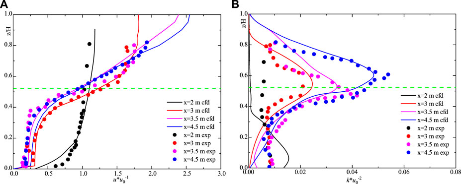
FIGURE 1. Comparison of numerical simulation and model test: (A) dimensionless velocity and (B) dimensionless turbulent kinetic energy.

3.2 Wave Through Emergent Vegetation

Based on wave flume, Lovas studied the effects of vegetation on wave propagation with different incident breaking wave parameters in shallow water. The experimental wave flume is 40 m long and 0.6 m wide. The artificial seaweed is placed on the slope of 1:30, and the vegetation patch is 7.26 m long. The model terrain is shown in Figure 2A. The height and diameter of artificial seaweed are 0.2 and 0.025 m respectively, and the vegetation density is 1,200 stem/m². In this calculation, three conditions including four different incident wave heights, two incident wave periods, and two water depths are selected to verify the simulation accuracy of the model for broken wave propagation and the vegetation dissipation process. The parameters of incident wave in the test conditions are shown in Table 1. The JONSWAP spectrum was used in the model, and the vegetation resistance coefficient was calculated by the formula proposed in the study by Kothyari et al. (2009). An unstructured grid is used in the calculation domain, and the calculation step is set to 0.2 s.

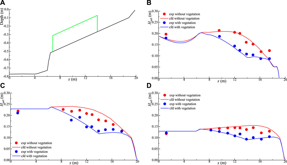
FIGURE 2. Comparison between numerical simulation and model test on the influence of vegetation patches on breaking wave height: (A) Bathymetry; (B) Case1; (C) Case2; and (D) Case3.

TABLE 1. Parameters of the incident wave in test condition.

The comparison of numerical simulation and model test on the influence of vegetation patches on breaking wave height is shown in Figure 2 above. The red data represent condition without vegetation, and the blue data represent condition with vegetation. It can be seen that in the process of wave propagation on the slope, the wave height decreases gradually. The wave energy dissipation provided by vegetation and topography contributes to the wave height attenuation, and the attenuation effect of vegetation on the wave is obvious. The results of numerical simulation are consistent with the experimental data under the three conditions, and the two sets of data are in good agreement, which indicates that the model can effectively simulate the propagation process of waves in vegetation patches.

4 Model Application

4.1 Study Area and Model Set up

Taihu Lake is located in the lower reaches of the Yangtze River Delta in Southeast China. It is the third largest freshwater lake in China, and its geographical location is shown in Figure 3. As a typical large shallow lake, the total area of Taihu Lake Basin is 36,900 m², the total area of Lake area is 2427.8 m², the average water depth is 1.9 m, and the maximum water depth is no more than 3 m. The Taihu Lake Basin has a subtropical monsoon climate, with an average annual rainfall of 1,200 mm, mainly in the monsoon season from May to September. Due to global warming and environmental pollution in recent years, algae blooms often occur in Taihu Lake, which has a devastating impact on the ecosystem (Jalil et al., 2019).

FIGURE 3. Geographical location of the study area, surrounding rivers, and monitoring points (where circular points are water-level verification points; square points are speed verification points; triangle points are wave height verification points).

The lake is connected to more than 150 rivers, many of which are seasonal. Because Taihu Lake is located in an area with strong human activities, a large number of water conservancy projects have made the inflow and outflow of the Lake strongly interfered by human activities. The main driving force of flow and wave field is wind. The dominant wind direction is southeast in summer and northwest in winter.

In recent years, the distribution and density of vegetation patches in Taihu Lake have changed with time, which affects the hydrodynamic characteristics, sediment, wave characteristics, and the stability of the lake ecosystem. The main vegetation types in Taihu Lake can be divided into submerged vegetation, emergent vegetation, and floating vegetation. Among them, submerged vegetation is dominated by Vallisneria natans and Ceratophyllum demersum L., emergent vegetation is dominated by Phragmites australis and Zizania latifolia, and floating vegetation is dominated by Potamogeton microdentatus. We used Vallisneria natans and Phragmites australis as the dominant of submerged vegetation and emergent vegetation, respectively, considering the influence of floating vegetation on the flow field of shallow lake is relatively small compared with the other two kinds of vegetation (Xu et al., 2018). In this study, only the effects of submerged vegetation and emergent vegetation on the characteristics of wind-driven current and wave are considered.

An unstructured grid is used in the computational domain. The horizontal grid consists of 1,25,433 cells and 59,386 nodes, and the size of the grid is between 30 and 150 m. The vertical grid is arranged in 30 layers according to the sigma coordinate, and the local refinement is carried out at the bottom and free surface. The average maximum depth slope of the grid is less than 0.33 to avoid the pressure gradient error caused by sigma transformation. The global calculation step is set to 1 s to satisfy the CFL stability condition. The model uses cold start and MURD (multidimensional upwind residual distribution scheme) scheme to deal with the convection and diffusion of variables.

The dataset of vegetation characteristics (regional distribution and density of vegetation) in the Taihu Lake region in 2016 was used in the numerical simulation, and the data were from the National Mathematical Center of Earth System Science of China (http://lake.geodata.cn/index.html); based on the Landsat remote sensing data in 2016, the image data of aquatic vegetation was obtained through band combination and image change technology, and the decision tree was constructed on the basis of the image data. Finally, the classification and density estimation results of aquatic vegetation were obtained. The regional distribution of vegetation in the Taihu Lake area is shown in Figure 4.

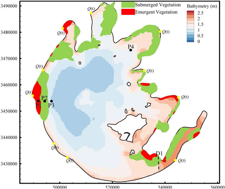
FIGURE 4. Regional distribution of vegetation in the Taihu Lake area. P1–P4 are the observation points, and D1 is the observation section of numerical simulation.

The input parameters of the vegetation model include the identification vector of each vegetation distribution area, resistance coefficient of vegetation, average height, and average width. The product of average height and average width is used to characterize the effective resistance area per unit volume of vegetation. Based on field investigation and the related literature (Wang et al., 2016), the density of submerged vegetation and emergent vegetation was set as 100 stem/m² and 150 stem/m², respectively, the average height of individual plant was set as 0.5 and 1.5 m, respectively, and the average width of individual plant was set as 0.007 and 0.015 m, respectively. The resistance coefficients of submerged vegetation and emergent vegetation are calculated through Hua’s research (Hua et al., 2013).

4.2 Model Verification

The data of 2016 were used to verify the numerical model. The average daily discharge of more than 150 tributaries connected with Taihu Lake in 2016 was generalized to 15 discharge boundaries as the driving force of the inflow and outflow of the lake (Liu et al., 2018); the daily rainfall evaporation data of VM1 station, hourly wind speed, and wind direction of WH1 station are collected as the atmospheric driving force of the model. Figure 5 shows the wind field data used to drive the model. For the treatment of bottom friction, the equivalent roughness is adopted, and 0.022 m is used for the whole bottom of the lake area. The background horizontal turbulence viscosity is set as 10^–4 m²/s, and the vertical turbulence viscosity is set as 10⁻⁶ m²/s.

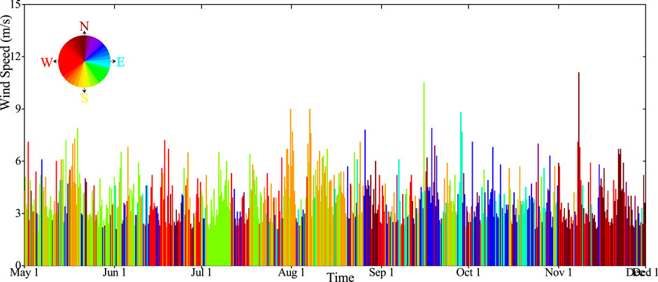
FIGURE 5. Wind speed and direction during calculation time.

In terms of model validation, hourly water level data of three stations from WL1 to WL3 during May 1 to December 1 were used to verify the water level results of hydrodynamic simulation. The surface velocity of VM1 and VM2 every 3 h from June 25 to 30 was used to verify the results. Daily wave height data from WH1 station from 29 May to 28 July were used to verify the results of wind wave simulation.

Figure 6 shows the simulated and observed data of the water level, velocity, and wave height of six stations, and the reliability of the calculated results is verified by RMSE and SS (Murphy, 1992). Even though the three water level monitoring points are located in different locations of the lake, the fluctuation of the water level shows a similar trend. This is because the water level of the lake is mainly regulated by tributary flow, rainfall, and evaporation. The wind speed has relatively little influence on the fluctuation of the water level. The velocity of VM1 and VM2, and the wave height of WH1 showed a similar trend to the wind speed, indicating that the flow field and wave field in Taihu Lake were mainly regulated by wind speed and direction, respectively. On the whole, the amplitude and phase of the water level, velocity, and wave obtained by simulation and observation are in good agreement.

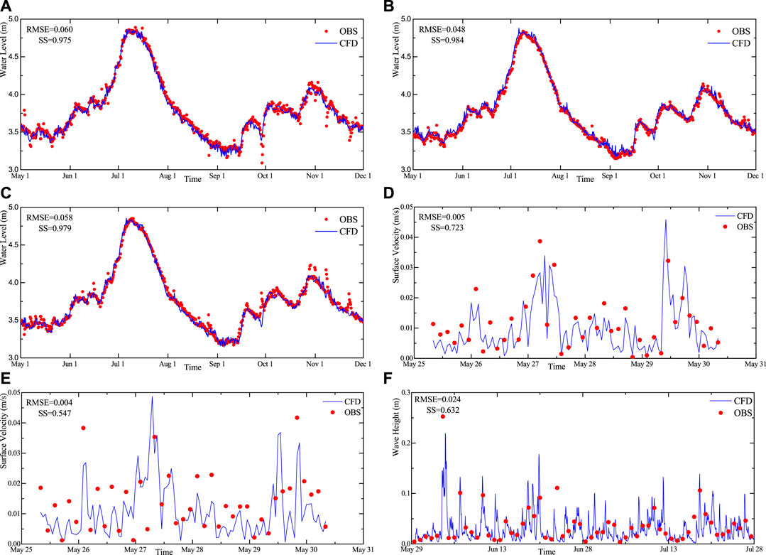
FIGURE 6. Comparison between numerical simulation results and observed data. (A) WL1, (B) WL2, (C) WL3, (D) VM1, (E) VM2, and (F) WH1.

4.3 The Effect of Vegetation on the Wind-Induced Current

Observed wind (see Figure 5) shows it could blow persistently at one prevailing direction for a couple of days until it changes direction, while the wind speed changes daily. Under the influence of stable wind direction, complex topography, and boundary of Taihu Lake, a variety of relatively stable circulation gyres will be formed in the lake after vertical averaging.

Figure 7 shows the depth-averaged flow field without the consideration of vegetation, and the velocity of the lake varies greatly in different regions. In the three northern bays, the structures of circulation gyres are similar where two small circulation gyres with opposite directions are formed. The direction of circulations near the entrances of the three bays is clockwise in July when the southeast wind is dominant and counterclockwise in November when the northwest wind is dominant. A slender circulation gyre has been formed along the west coast of the lake, and the average circulation direction is clockwise in July and counterclockwise in November. Several small-scale gyres with different sizes and directions appeared in the central region of the lake under the influence of the high velocity area in the southwest region and the topography of Xishan Island. By comparing the average circulation patterns of Taihu Lake in July and November, it can be seen that the circulation characteristics are similar but the circulation direction is opposite under the influence of different directions of dominant wind (Li et al., 2011).

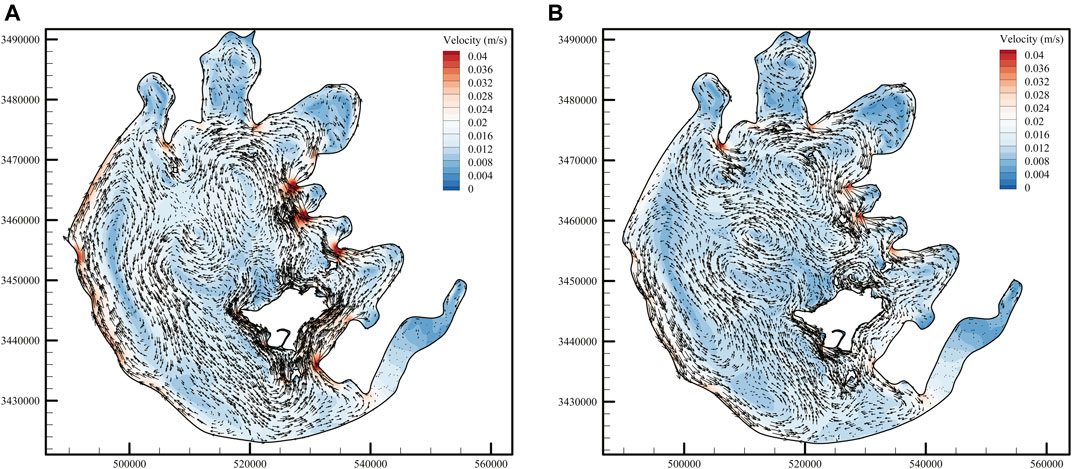
FIGURE 7. Monthly mean depth-averaged flow field without the consideration of vegetation: (A) July and (B) November.

Figure 8 shows the depth-averaged flow field with the consideration of vegetation. Due to the blockage effect of vegetation, the flow velocity decreases significantly in the lake area with vegetation, and increases to a certain extent in the vicinity of vegetation patches due to the agglomeration of kinetic energy (Tse et al., 2016). The vegetation patches distributed at the entrance of Zhushan Bay and the central part of Meiliang Bay reduces the local current velocity and the water exchange capacity with the central area. Due to the existence of large areas of submerged vegetation and emergent vegetation, the current velocity decreases near the southwest bank of Taihu Lake, thus changing the structure of slender circulation in this region. At the entrance of Dongtaihu Bay, the flow velocity at the vegetation patches on the north side decreased sharply. Due to the narrow bay, the kinetic energy was tightly surrounded by the vegetation patches and the north side, so the flow velocity in this area increased significantly compared with that without considering the vegetation. In summary, it is found that the circulation characteristic of the lake in the two cases is similar, regardless of whether the influence of vegetation is considered, but the circulation structure of the vegetation patch and its vicinity will change significantly.

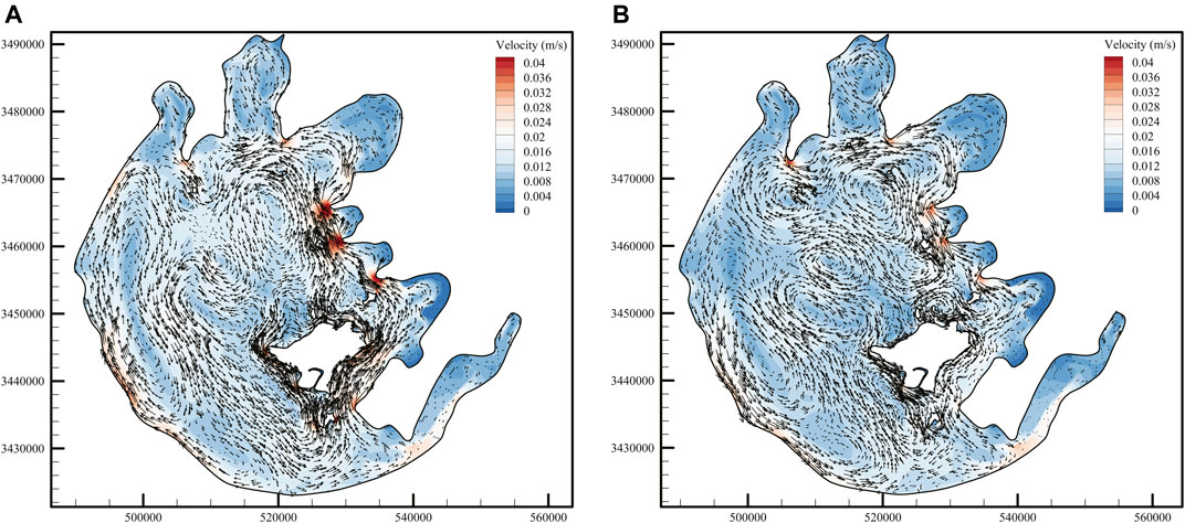
FIGURE 8. Monthly mean depth-averaged flow field with the consideration of vegetation: (A) July and (B) November.

Figure 9 shows the temporal variation of the velocity difference among the three monitoring points. Among them, P1 is located in the emergent vegetation patch near the west bank of the lake, P2 is located in the submerged vegetation patch, and P3 is located in the non-vegetation area, affected by the topography of Taihu Lake and local wind field; the area where the three points are located is prone to elongated circulation gyre near the west shore (see Figure 7). The velocity difference of P1 is greater than that of P2, indicating that the blocking effect of emergent vegetation is stronger than that of submerged vegetation. The velocity difference of P3 is mostly less than 0, which is due to the redistribution of kinetic energy caused by the influence of vegetation obstruction near the west coast. As a result, the flow velocity in this region with vegetation is greater than that without vegetation. Meanwhile, when the velocity difference of P1 is large, the velocity difference of P2 and P3 is also large.

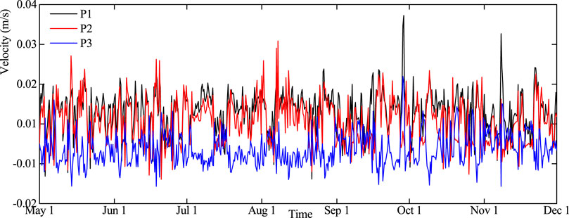
FIGURE 9. Time variation of velocity difference at monitoring points; positive values in the figure indicate that the flow velocity under the condition of without vegetation is higher than that under the condition of with vegetation.

Figure 10 shows the vertical flow field of the cross section shown by the dotted line in the figure. The submerged vegetation is distributed on the north side of the entrance of Dongtaihu Bay (see the green dotted line in Figure 4B). In the absence of vegetation, due to the shear action of wind stress, the flow velocity on the free surface is higher than that at the bottom. Meanwhile, influenced by the circulation and the compensation flow at the bottom, the section forms a clockwise secondary flow, and the average velocity on the north side of the section is higher than that on the south side. When considering the influence of vegetation, the flow velocity of vegetation patch decreases due to the blocking effect of vegetation. The average velocity on the north side of the section decreased, while the velocity on the south side of the section increased significantly due to the redistribution of kinetic energy, which was much higher than that without considering the influence of vegetation. The presence of local vegetation patches changed the secondary flow characteristics of the section. Episodic shear flow over the top of the vegetation has a capacity to redistribute constituents and organisms positioned deeply within the vegetation, remote from open water (Abdul et al., 2017a).

FIGURE 10. Vertical velocity distribution of the section of Dongtaihu Bay in July; green dots in the figure represent vegetation patches. (A) Without vegetation and (B) with vegetation.

4.4 The Effect of Vegetation on the Wind-Induced Wave

Figure 11 shows the average wave height distribution of the lake in July with and without the consideration of vegetation, and the simulation results of other monthly averages are similar to the figure, so they will not be repeated. As shown in Figure 11A, the high wave height mainly occurs in the areas with large wind blowing fetch and deep water depth. Comparing the distribution of wave height and the topography of Taihu Lake, it can be seen that the area with the maximum water depth is very similar to the area with the maximum wave height. Figure 11B shows the wave height distribution with the consideration of vegetation. It can be seen that there is no obvious change in the wave height of submerged vegetation patches. Under the influence of blocking effect of emergent vegetation, the wave height on the west bank and the north bank of the entrance of Dongtaihu Bay decreased significantly; this is because the resistance coefficient, vegetation height, and the width of submerged vegetation are much lower than those of emergent vegetation, making the ability of submerged vegetation to reduce wind-induced wave worse than that of emergent vegetation. The simulation results show that emergent vegetation has the potential to provide coastline protection by reducing wave height.

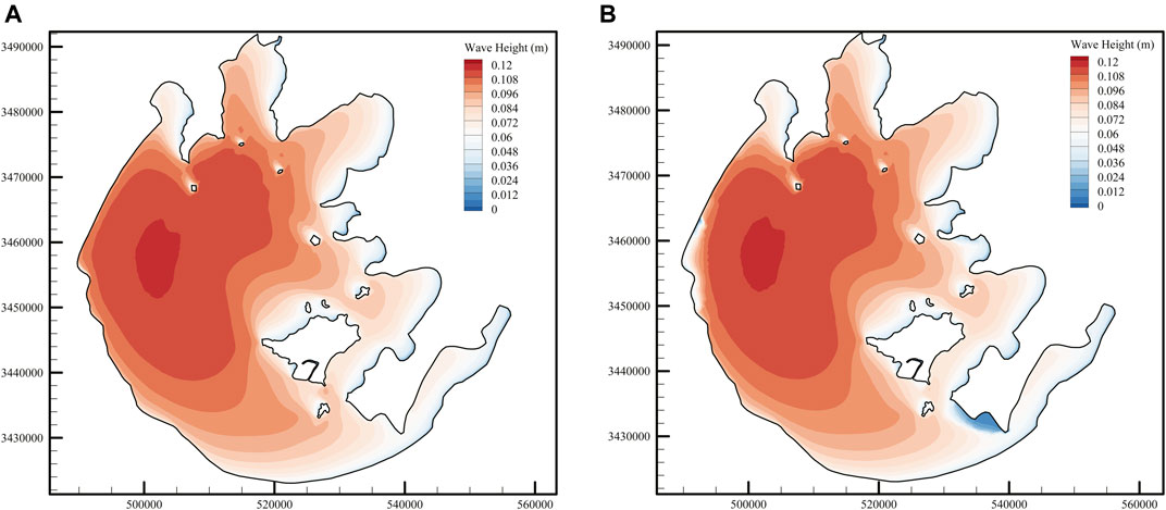
FIGURE 11. Average wave height distribution of Taihu Lake with and without vegetation in July. (A) Without vegetation and (B) with vegetation.

Figure 12 shows the time sequence changes of wave height difference at monitoring points P1 and P2. It can be seen from the figure that the wave height difference at the emergent vegetation patch is much higher than that at the submerged vegetation patch (Parvathy et al., 2017). According to Figure 5, when the wind direction is southeast and lasts for a long time, the wind blowing fetch and wave height of P1 and P2 points are larger, and the larger the incident wave height is, the more obvious the wave height attenuation of vegetation water area is. Therefore, it is feasible to protect the lake bank embankment project by arranging appropriate emergent vegetation patches on the west bank of the lake to reduce the high wind-induced wave caused by typhoons in summer.

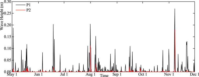
FIGURE 12. Time variation of wave height difference at monitoring points; positive values in the figure indicate that the wave height under the condition of without vegetation is higher than that under the condition of with vegetation.

4.5 The Effects of Vegetation on Material Transport Characteristics

In order to study the influence of vegetation on the material transport characteristics of Taihu Lake, the tracer was continuously released at the inlet of Wangyu River at the amount of 1 kg/s, and the initial tracer concentration in the calculation domain was set to 0. Here, in this study, depth-averaged tracer concentration is presented. Figure 13 shows the concentration distribution of the tracer in the lake at different times without the consideration of vegetation; after leaving Gonghu Bay, the tracer entered the central area of the lake and was mixed into these bays due to the influence of small-scale circulation gyres. As the dominant wind direction in July was opposite to that in November, the high tracer concentration area in Taihu Lake was located in the northwest region under the dominance of southeast wind in July, while the high tracer concentration area under the dominance of northwest wind in November was located in the southeast region. Combined with the monthly mean flow field in Taihu Lake shown in Figure 7, it has been found that the transport characteristics of tracer in Taihu Lake are mainly controlled by different circulation structures under the influence of different wind directions.

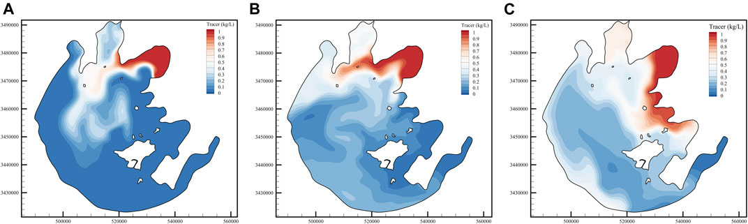
FIGURE 13. Time series of tracer concentration images without the consideration of vegetation: (A) Jul, 31st, (B) Sept, 30th, and (C) Nov, 30th.

Figure 14 shows the concentration distribution of the tracer in the lake at different times with the consideration of vegetation. Combined with Figures 13, 15, it can be seen that vegetation can “delay” the transport of the tracer. For example, without the consideration of vegetation, tracers have been spread throughout the whole Gonghu Bay on 30 July, and covered most of the Zhushan Bay. With the consideration of vegetation, the concentration of the tracer in the southern part of Gonghu Bay and the northern part of Zhushan Bay decrease significantly. No significant difference is found in the concentration of tracer in the two regions, whether vegetation is considered or not on 30 September. These conditions also occur on the west bank of the lake on 30 September and in the Xukou Bay area on 30 November. The area with large concentration difference of tracer gradually evolves from the three northern bays to the southwest region of Taihu Lake, which is related to the mainstream movement direction of the tracer. The maximum difference of tracer concentration at different times can reach 0.29 kg/s, and the tracer area under the condition of considering vegetation is smaller than that without considering vegetation. The main reason for the difference in tracer concentration is due to the blocking effect of vegetation, which reduces the local velocity and changes the circulation structure, thus affecting the convection and diffusion of the tracer. In summary, the presence of vegetation reduces the exchange rate between vegetation patches and the outside world, and has an important effect on the material transport characteristics of the lake.

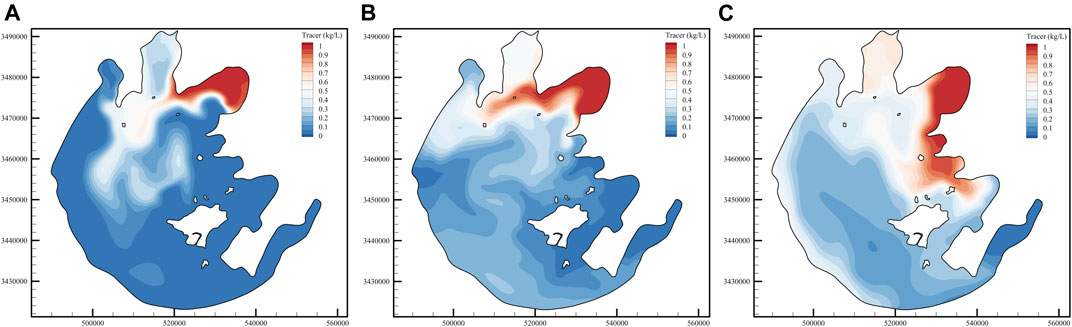
FIGURE 14. Time series of tracer concentration images with the consideration of vegetation: (A) Jul, 31st, (B) Sept, 30th, and (C) Nov, 30th.

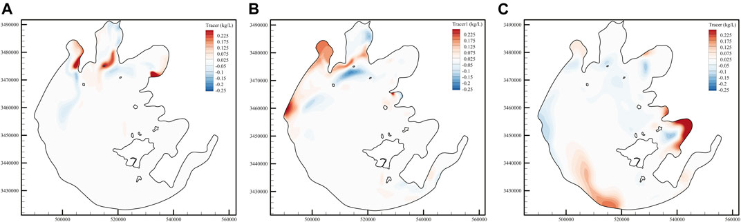
FIGURE 15. Spatial influence of vegetation on tracer concentration; positive values in the figure indicate that the tracer concentration under the condition of without vegetation is higher than that under the condition of with vegetation. (A) Jul, 31st, (B) Sept, 30th, and (C) Nov, 30th.

4.6 Sensitivity Analysis

In the vegetation resistance term, density, height, and diameter of vegetation largely determine the resistance per unit area. In different seasons, the density, height, and diameter of each vegetation patch in the lake are different, but most of the models use constant values that do not change with time and space, which is bound to have a great impact on the results.

In order to study the effects of different vegetation parameter values on the characteristics of wind-induced wave and current in Taihu Lake, sensitivity analysis was conducted for vegetation density in this section. The reference density (150 stem/m² for emergent vegetation and 100 stem/m² for submerged vegetation) was n = 1.0 and n = 0 for the absence of vegetation. Figure 16 shows the influence of different vegetation densities on the results. With the gradual increase of vegetation density, the velocity of P1 gradually decreases. Meanwhile, due to the redistribution of kinetic energy, the velocity of P3 increases, and the trend of decreasing or rising velocity flattens out with the increase of vegetation density. Similar effects also appear in the simulation of wave height. The wave height at P1 and P2 decreases with the increase of vegetation density, and the decreasing trend of velocity gradually flattens out. Meanwhile, the decreasing gradient of wave height at P1 is much lower than that of P1, indicating that the capacity of emergent vegetation to reduce wind-induced wave is greater than that of submerged vegetation. As can be seen from Figure 16C, the concentration of the tracer at P1 point showed a trend of gradual increase and then decrease over time without the consideration of vegetation. In the case of considering the influence of vegetation, the change of tracer concentration at P1 is similar to that without considering vegetation, but the inflection point (the point where tracer concentration changes from an upward trend to a downward trend) appears later, and the maximum tracer concentration decreases. With the gradual increase of vegetation density, the inflection point appeared later, and the maximum concentration of tracer gradually decreased. Even if the overall vegetation density is reduced to 25% of the reference density (37.5 stem/m² for emergent vegetation and 25 stem/m² for submerged vegetation), the results of the wind-induced wave and current characteristics of shallow lakes with the consideration of vegetation are significantly different from those without the consideration of vegetation. Therefore, the influence of vegetation should not be ignored in the numerical simulation of lake dynamics.

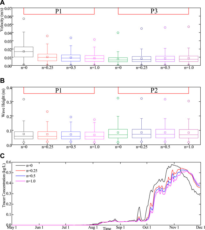
FIGURE 16. Sensitivity analysis of the influence of vegetation density on the results: (A) sensitivity analysis of velocity at P1 and P3, (B) sensitivity analysis of wave height at P1 and P2, and (C) sensitivity analysis of tracer concentration at P1.

5 Discussion

As a typical eutrophic lake, the algae bloom usually exists in Taihu Lake, which is closely related to the characteristics of wind-induced wave and current (Abdul et al., 2017b). The nutrients would be transported due to strong wind-induced current. At the same time, wind waves are also conducive to the re-suspension of the sediment and to promote the release of nutrients from the sediment. The model application in Section 4 shows the applicability of the flow–wave–vegetation coupling model in the numerical simulation of shallow lakes with vegetation patches. The results show that the presence of vegetation patches significantly changes the characteristics of the wind-induced wave, current, and material transport in shallow lakes. This shows that the layout of submerged and emergent vegetation patches in appropriate areas can change the lake hydrodynamic structure in local areas where algae bloom usually occurs, so as to reduce the probability of algae bloom. These results provide meaningful information for the study of long-term vegetation evolution in shallow lakes.

However, the flow–wave–vegetation coupling model established above has some limitations and uncertainties. Different from the similar and evenly distributed vegetation in the laboratory, the vegetation parameters in the natural environment are often uncertain, and the vegetation types, growth degree, density, project area, and drag coefficient in different regions are often different (Li et al., 2020). At present, methods such as NDVI estimation (Adamala et al., 2016) and field sampling have been widely used to retrieve vegetation parameters in shallow lakes. But the error of observation and the different choice of the calculation model will lead to the different results of vegetation parameters under different schemes (Lamchin et al., 2020). As shown in the sensitivity analysis in Section 4.6, there are obvious differences in the wind-induced wave, current, and material transport characteristics with different vegetation densities (Smith et al., 2016), but these vegetation parameters are often roughly summarized in mathematical models (Weiming and Marsooli, 2012); for example, the vegetation density in the whole vegetation patch is set to the same value (although the vegetation density in different areas of the same vegetation patch is different); this leads to the distortion of the calculation results. In the future, it is necessary to refine the resistance module of vegetation, so as to make the calculation results of the model closer to the real situation.

Meanwhile, the application of the flow–wave–vegetation coupling model also touches the challenge of simulating the long-term and large-scale vegetation growth and attenuation process. The distribution and parameters of vegetation patches will change periodically with different seasons, but the coupling model does not take into account the response of vegetation to nutrients, light intensity, and suspended sediment concentration, so it cannot simulate the process of vegetation growth and attenuation (Cerco and Moore, 2001). The AED model (http://aed.see.uwa.edu.au/research/models/AED/) is coupled with the Open TELEMAC-MASCARET model; the model takes into account the carbon, nitrogen, and phosphorus cycles, as well as the effects of other related factors such as dissolved oxygen, light, and suspended sediment, and can simulate the biochemical process and ecological function among phytoplankton, zooplankton, and environment. We can refer to the Cai (2018) method in the future, by splitting vegetation parameters into leaves, roots, and stems, and parameterizing their relationships with variables such as water quality, light intensity, and suspended sediment concentration; coupling the response among vegetation, hydrodynamic force and wave, and the response between vegetation parameters and ecological action, a complete ecological model was established to consider the impact of vegetation on wind-induced wave and current. The fully coupled model can be used to simulate the algae bloom and ecological processes in shallow lakes. The vegetation module based on the Open TELEMAC-MASCARET in this article can provide some reference for such research.

6 Conclusion

Based on the Open TELEMAC-MASCARET model, we implanted the vegetation module into the 3d flow model TELEMAC-3D and the wave model TOMAWAC, respectively, and built the flow–wave–vegetation coupling model. Through two sets of laboratory data verification, it has been proven that the model can well capture the complex three-dimensional flow structure and turbulent characteristics near vegetation patches, and accurately predict the attenuation characteristics of waves in the waters with vegetation patches. The model was then applied to the simulation of wind-induced wave and current in Taihu Lake, a typical shallow lake. By comparing the calculated results with the measured data, it has been shown that the model can accurately reproduce the long-term wind-induced wave and current characteristics of shallow lakes. It is found that vegetation has a significant effect on the velocity of the vegetation patch and its adjacent area, and also changes the three-dimensional circulation structure, so as to redistribute constituents and organisms positioned deeply within the vegetation, remote from open water. The resistance of emergent vegetation is higher than that of submerged vegetation, and the attenuation ability of wave is also stronger than that of submerged vegetation. The presence of vegetation reduces the exchange rate between vegetation patches and the outside area, and has an important effect on the material transport characteristics of the lake. The change of velocity and wave height gradually flattens out with the increase of vegetation density, and the sensitivity analysis results show that the influence of vegetation should not be ignored in the numerical simulation of hydrodynamic lake. This model helps to better understand the impact of aquatic vegetation on the natural environment and provides a useful tool for decision-making on the potential ecological benefits of aquatic vegetation.

Data Availability Statement

The raw data supporting the conclusion of this article will be made available by the authors, without undue reservation.

Author Contributions

All authors listed have made a substantial, direct and intellectual contribution to the work and approved it for publication.

Funding

This work was jointly funded by the National Key R&D Program of China (2018YFC0407200) and the Special Research Fund of the Nanjing Hydraulic Research Institute (Y120010).

Conflict of Interest

The authors declare that the research was conducted in the absence of any commercial or financial relationships that could be construed as a potential conflict of interest.

Publisher’s Note

All claims expressed in this article are solely those of the authors and do not necessarily represent those of their affiliated organizations, or those of the publisher, the editors and the reviewers. Any product that may be evaluated in this article, or claim that may be made by its manufacturer, is not guaranteed or endorsed by the publisher.

References

Abdul, J., Yiping, L., Wei, D., Jianwei, W., Xiaomeng, G., Wencai, W., et al. (2017). Wind-Induced Flow Velocity Effects on Nutrient Concentrations at Eastern Bay of Lake Taihu, China. Environ. Sci. Pollut. Res. 24, 17900–17911. doi:10.1007/s11356-017-9374-x
Abdul, J., Yiping, L., Du, W., Wencai, W., Jianwei, W., Xiaomeng, G., et al. (2017). The Role of Wind Field Induced Flow Velocities in Destratification and Hypoxia Reduction at Meiling Bay of Large Shallow Lake Taihu, China. Environ. Pollut. 232, 591–602. doi:10.1016/j.envpol.2017.09.095
Adamala, S., Rajwade, Y. A., and Reddy, Y. V. K. (2016). Estimation of Wheat Crop Evapotranspiration Using NDVI Vegetation index. J. Appl. Nat. Sci. 8 (1), 159–166. doi:10.31018/jans.v8i1.767
Bacchi, V., Gagnaire, E., Durand, N., and Benoit, M. (2014). “Wave Energy Dissipation by Vegetation in TOMAWAC,” in XXIst Telemac-Mascaret User Conference, Grenoble, France, 15–17 October, 2014.
Banerjee, T., Muste, M., and Katul, G. (2015). Flume Experiments on Wind Induced Flow in Static Water Bodies in the Presence of Protruding Vegetation. Adv. Water Resour. 76, 11–28. doi:10.1016/j.advwatres.2014.11.010
Barbier, E. B., Koch, E. W., Silliman, B. R., Hacker, S. D., Wolanski, E., Primavera, J., et al. (2008). Coastal Ecosystem-Based Management with Nonlinear Ecological Functions and Values. Science 319 (5861), 321–323. doi:10.1126/science.1150349
Beudin, A., Kalra, T., Ganju, N., and Warner, J. C. (2017). Development of a Coupled Wave-Flow-Vegetation Interaction Model. Comput. Geosciences 100, 76–86. doi:10.1016/j.cageo.2016.12.010
Cai, X. (2018). Impact of Submerged Aquatic Vegetation on Water Quality in Cache Slough Complex, Sacramento-San Joaquin Delta- A Numerical Modeling Study. Sacramento, CA: The College of William and Mary in Virginia.
Cerco, C. F., and Moore, K. (2001). System-Wide Submerged Aquatic Vegetation Model for Chesapeake Bay. Estuaries 24 (4), 522–534. doi:10.2307/1353254
Chi-wai, L., and Afis, O. B. (2019). Hybrid Modeling of Flows Over Submerged Prismatic Vegetation with Different Areal Densities. Eng. Appl. Comput. Fluid Mech. 13 (1), 493–505. doi:10.1080/19942060.2019.1610501
Dan, W., and Hua, Z. (2014). The Effect of Vegetation on Sediment Resuspension and Phosphorus Release under Hydrodynamic Disturbance in Shallow Lakes. Ecol. Eng. 69, 55–62. doi:10.1016/j.ecoleng.2014.03.059
Gaylord, B., Denny, M. W., and Koehl, M. A. R. (2003). Modulation of Wave Forces on Kelp Canopies by Alongshore Currents. Limnol. Oceanogr. 48 (2), 860–871. doi:10.4319/lo.2003.48.2.0860
Hervouet, J.-M. (2007). Hydrodynamics of Free Surface Flows: Modelling with the Finite Element Method. West Sussex, UK: Wiley, 360.
Hua, Z., Wu, D., Kang, B., and Li, Q. (2013). Flow Resistance and Velocity Structure in Shallow Lakes with Flexible Vegetation under Surface Shear Action. J. Hydraul. Eng. 139, 612–620. doi:10.1061/(asce)hy.1943-7900.0000712
Jalil, A., Li, Y., Zhang, K., Gao, X., Wang, W., Khan, H. O. S., et al. (2019). Wind-Induced Hydrodynamic Changes Impact on Sediment Resuspension for Large, Shallow Lake Taihu, China. Int. J. Sediment Res. 34 (3), 205–215. doi:10.1016/j.ijsrc.2018.11.003
Jin, K.-R., Ji, Z.-G., and James, R. T. (2007). Three-Dimensional Water Quality and SAV Modeling of a Large Shallow Lake. J. Great Lakes Res. 33 (1), 28–45. doi:10.3394/0380-1330(2007)33[28:twqasm]2.0.co;2
Karim, F., Dutta, D., Marvanek, S., Petheram, C., Ticehurst, C., Lerat, J., et al. (2015). Assessing the Impacts of Climate Change and Dams on Floodplain Inundation and Wetland Connectivity in the Wet-Dry Tropics of Northern Australia. J. Hydrol. 522, 80–94. doi:10.1016/j.jhydrol.2014.12.005
Kim, H. S., Nabi, M., Kimura, I., and Shimizu, Y. (2015). Computational Modeling of Flow and Morphodynamics through Rigid-Emergent Vegetation. Adv. Water Resour. 84, 64–86. doi:10.1016/j.advwatres.2015.07.020
King, A. T., Tinoco, R. O., and Cowen, E. A. (2012). A K-ε Turbulence Model Based on the Scales of Vertical Shear and Stem Wakes Valid for Emergent and Submerged Vegetated Flows. J. Fluid Mech. 701, 1–39. doi:10.1017/jfm.2012.113
Kombiadou, K., Ganthy, F., Verney, R., Plus, M., and Sottolichio, A. (2014). Modelling the Effects of Zostera Noltei Meadows on Sediment Dynamics: Application to the Arcachon Lagoon. Ocean Dyn. 64 (10), 1–18. doi:10.1007/s10236-014-0754-1
Kothyari, U. C., Hashimoto, H., and Hayashi, K. (2009). Effect of Tall Vegetation on Sediment Transport by Channel Flows. J. Hydraulic Res. 47 (6), 700–710. doi:10.3826/jhr.2009.3317
Lamchin, M., Wang, W., Lim, C.-H., Ochir, A., Ukrainski, P., Gebru, B., et al. (2020). Understanding Global Spatio-Temporal Trends and the Relationship between Vegetation Greenness and Climate Factors by Land Cover during 1982-2014. Glob. Ecol. Conservation 24, e01299. doi:10.1016/j.gecco.2020.e01299
Large, W. G., and Pond, S. (1981). Open Ocean Momentum Flux Measurements in Moderate to Strong Winds. J. Phys. Oceanography 11 (3), 336–342. doi:10.1175/1520-0485(1981)011<0324:oomfmi>2.0.co;2
Li, Y., Acharya, K., and Yu, Z. (2011). Modeling Impacts of Yangtze River Water Transfer on Water Ages in Lake Taihu, China. Ecol. Eng. 37 (2), 325–334. doi:10.1016/j.ecoleng.2010.11.024
Li, Y., Teng, Y.-C., Kelly, D. M., and Zhang, K. (2016). A Numerical Study of the Impact of hurricane-induced Storm Surge on the Herbert Hoover Dike at Lake Okeechobee, Florida. Ocean Dyn. 66 (12), 1699–1714. doi:10.1007/s10236-016-1001-8
Li, Y., Zhang, Q., Tan, Z., and Yao, J. (2020). On the Hydrodynamic Behavior of Floodplain Vegetation in a Flood-Pulse-Influenced River-lake System (Poyang Lake, China). J. Hydrol. 585, 124852. doi:10.1016/j.jhydrol.2020.124852
Liu, S., Ye, Q., Wu, S., and Stive, M. (2018). Horizontal Circulation Patterns in a Large Shallow Lake: Taihu Lake, China. Water 10, 1–27. doi:10.3390/w10060792
Løvås, S. M. (2000). Hydro-physical Conditions in Kelp Forests and the Effect on Wave Dumping and Dune Erosion: A Case Study on Laminaria Hyperborea. Norway: University of Trondheim.
Lu, J., and Dai, H. C. (2017). Three Dimensional Numerical Modeling of Flows and Scalar Transport in a Vegetated Channel. J. Hydro-Environment Res. 16, 27–33. doi:10.1016/j.jher.2017.05.001
Lürling, M., Mackay, E., Reitzel, K., and Spears, B. M. (2016). Editorial - A Critical Perspective on Geo-Engineering for Eutrophication Management in Lakes. Water Res. 97, 1–10. doi:10.1016/j.watres.2016.03.035
Morales-Marín, L. A., French, J. R., and Burningham, H. (2017). Implementation of a 3D Ocean Model to Understand upland lake Wind-Driven Circulation. Environ. Fluid Mech. 17, 1255–1278. doi:10.1007/s10652-017-9548-6
Morin, J., Leclerc, M., Secretan, Y., and Boudreau, P. (2000). Integrated Two-Dimensional Macrophytes-Hydrodynamic Modeling. J. Hydraulic Res. 38 (3), 163–172. doi:10.1080/00221680009498334
Murphy, A. H. (1992). Climatology, Persistence, and Their Linear Combination as Standards of Reference in Skill Scores. Wea. Forecast. 7 (4), 692–698. doi:10.1175/1520-0434(1992)007<0692:cpatlc>2.0.co;2
Nepf, H. M. (2011). Flow and Transport in Regions with Aquatic Vegetation. Annu. Rev. Fluid Mech. 44 (1), 123–142. doi:10.1146/annurev-fluid-120710-101048
Neumeier, U. (2007). Velocity and Turbulence Variations at the Edge of Saltmarshes. Continental Shelf Res. 27, 1046–1059. doi:10.1016/j.csr.2005.07.009
Pang, C.-C., Wang, F., Wu, S.-Q., and Lai, X.-J. (2015). Impact of Submerged Herbaceous Vegetation on Wind-Induced Current in Shallow Water. Ecol. Eng. 81 (8), 387–394. doi:10.1016/j.ecoleng.2015.04.021
Parvathy, K. G., Umesh, P. A., and Bhaskaran, P. K. (2017). Inter-seasonal Variability of Wind-Waves and Their Attenuation Characteristics by Mangroves in a Reversing Wind System. Int. J. Climatology 37 (c4), 5089–5106. doi:10.1002/joc.5147
Resende, A. F. d., Schöngart, J., Streher, A. S., Ferreira-Ferreira, J., Piedade, M. T. F., and Silva, T. S. F. (2019). Massive Tree Mortality from Flood Pulse Disturbances in Amazonian Floodplain Forests: The Collateral Effects of Hydropower Production. Sci. Total Environ. 659, 587–598. doi:10.1016/j.scitotenv.2018.12.208
Sheng, Y. P., Lapetina, A., and Ma, G. (2012). The Reduction of Storm Surge by Vegetation Canopies: Three-Dimensional Simulations. Geophys. Res. Lett. 39 (20), 1–5. doi:10.1029/2012gl053577
Smith, J. M., Bryant, M. A., and Wamsley, T. V. (2016). Wetland Buffers: Numerical Modeling of Wave Dissipation by Vegetation. Earth Surf. Process. Landforms 41 (6), 847–854. doi:10.1002/esp.3904
Sonnenwald, F., Guymer, I., and Stovin, V. (2019). A CFD‐Based Mixing Model for Vegetated Flows. Water Resour. Res. 55 (3), 2322–2347. doi:10.1029/2018wr023628
Temmerman, S., Meire, P., Bouma, T. J., Herman, P. M. J., Ysebaert, T., and De Vriend, H. J. (2013). Ecosystem-Based Coastal Defence in the Face of Global Change. Nature 504 (7478), 79–83. doi:10.1038/nature12859
Tse, I. C., Poindexter, C. M., and Variano, E. A. (2016). Wind-Driven Water Motions in Wetlands with Emergent Vegetation. Water Resour. Res. 52, 2571–2581. doi:10.1002/2015wr017277
Vossen, B. V., and Uittenbogaard, R. (2004). “Subgrid-Scale Model for quasi-2D Turbulence in Shallow Water,” in Shallow Flows. London, UK: Taylor & Francis Group. doi:10.1201/9780203027325.ch72
Wang, C., Fan, X.-l., Wang, P.-f., Hou, J., and Qian, J. (2016). Flow Characteristics of the Wind-Driven Current with Submerged and Emergent Flexible Vegetations in Shallow Lakes. J. Hydrodyn 28 (5), 746–756. doi:10.1016/s1001-6058(16)60677-7
Weiming, W., and Marsooli, R. (2012). A Depth-Averaged 2D Shallow Water Model for Breaking and Non-Breaking Long Waves Affected by Rigid Vegetation. J. Hydraulic Res. 50 (6), 558–575. doi:10.1080/00221686.2012.734534
Werner, M. G. F., Hunter, N. M., and Bates, P. D. (2005). Identifiability of Distributed Floodplain Roughness Values in Flood Extent Estimation. J. Hydrol. 314, 139–157. doi:10.1016/j.jhydrol.2005.03.012
Xu, T.-P., Zhang, M.-L., Jiang, H.-Z., Tang, J., Zhang, H.-X., and Qiao, H.-T. (2018). Numerical Investigation of the Effects of Aquatic Plants on Wind-Induced Currents in Taihu Lake in China. J. Hydrodyn 31, 778–787. doi:10.1007/s42241-018-0091-9
Yang, P., Fong, D. A., Lo, E. Y. M., and Monismith, S. G. (2019). Circulation Patterns in a Shallow Tropical Reservoir: Observations and Modeling. J. Hydro-environment Res. 27, 75–86. doi:10.1016/j.jher.2019.09.002
Zhang, J., Fan, X., Liang, D., and Liu, H. (2019). Numerical Investigation of Nonlinear Wave Passing through Finite Circular Array of Slender Cylinders. Eng. Appl. Comput. Fluid Mech. 13, 102–116. doi:10.1080/19942060.2018.1557561
Keywords: aquatic vegetation, flow–wave–vegetation coupling model, shallow lake, wind-induced wave and current, Open TELEMAC-MASCARET
Citation: Wu C, Wu S, Wu X, Dai J, Gao A and Yang F (2022) Numerical Investigation of the Effects of Aquatic Vegetation on Wind-Induced Wave and Current Characteristics in Shallow Lakes. Front. Environ. Sci. 9:829376. doi: 10.3389/fenvs.2021.829376
Received: 05 December 2021; Accepted: 30 December 2021;
Published: 24 January 2022.
Edited by:
Yuanchun Zou, Northeast Institute of Geography and Agroecology (CAS), ChinaReviewed by:
Ronghua Ma, Nanjing Institute of Geography and Limnology (CAS), ChinaAbdul Jalil, Wuxi University, China
Copyright © 2022 Wu, Wu, Wu, Dai, Gao and Yang. This is an open-access article distributed under the terms of the Creative Commons Attribution License (CC BY). The use, distribution or reproduction in other forums is permitted, provided the original author(s) and the copyright owner(s) are credited and that the original publication in this journal is cited, in accordance with accepted academic practice. No use, distribution or reproduction is permitted which does not comply with these terms.
*Correspondence: Shiqiang Wu, sqwu@nhri.cn; Xiufeng Wu, xfwu@nhri.cn; Jiangyu Dai, jydai@nhri.cn