Wind turbines as a metamaterial-like urban layer: an experimental investigation using a dense seismic array and complementary sensing technologies

1 Introduction

The interactions between the soil and urban structures above it can strongly modify seismic ground motion, as first outlined by Jennings and Kuroiwa (1968) and Luco and Contesse (1973). Following the 1985 Michoacán (Mexico) earthquake, due to the difficulties of traditional computational approaches in matching seismic records, Wirgin and Bard (1996) proposed that some of the seismic energy transmitted to the buildings is redistributed in their surroundings through numerous structure-soil-structure interactions. This phenomenon was called “site-city interaction” or “city effect”. Following this study, a number of authors have investigated the possible feedback of the soil-structure interaction on the free-field ground motion with a special focus on densely urbanized areas. These studies involved either numerical simulations based on more or less detailed soil properties and/or structural characteristics (e.g., Guéguen et al., 2002; Tsogka and Wirgin, 2003; Kham et al., 2006; Schwan et al., 2016) as well as laboratory experiments at a reduced scale based on shaking tables or acoustic devices (e.g., Mason et al., 2013; Tian et al., 2023). The majority of them yield consistent results showing the possibility of observable effects on seismic ground motion with an overall decrease in the average level of ground motion at specific frequency ranges with greater spatial variability.

In this sense, the emergence of the so-called metamaterial-like concept in the urban fabric is a promising prospect to be developed. Typically, a metamaterial is based either on the periodic arrangement or on the resonant properties of elements with their dimension being much smaller than the wavelength considered (typically λ/2 to λ/10). As a result, these materials acquire effective properties not observed in constituent materials. Metamaterials have expanded the variety of options for influencing and directing wave propagation including ultrasound, acoustic, thermodynamic, electromagnetic and elastic waves (reviews provided by Simovski, 2009; Kadic et al., 2013; 2019; Turpin et al., 2014; Kumar et al., 2022; Qahtan et al., 2022 among others). Although these mentioned topics deal with different kinds of waves, analogies between them can still be drawn.

For applications in seismology, the innovative work of Liu et al. (2000) on locally resonant crystals with structural periodicity two orders of magnitude smaller than the respective sonic wavelength and exhibiting clear bandgaps clears the way for the damping of Rayleigh waves within the sub-wavelength regime. Following on from this study, experiments ranging from optical wave manipulation to acoustic testing have been used to study the underlying nature and resilience of metamaterial physics. Common vibration mitigation measures that have been proposed include the use of rows of piles (Avilés and Sánchez-Sesma, 1988; Gao et al., 2006; Dijckmans et al., 2016), open or infill trenches (Dasgupta et al., 1990; Laghfiri and Lamdouar, 2022) and wave impeding barrier. Regarding the first issue, Brule et al. (2014) explored the impact of a periodic arrangement of pile foundations in soft soils as a seismic barrier as if it was a giant crystal. The authors have demonstrated that boreholes with meter-long spacing can attenuate seismic surface waves in the Bragg scattering regime, achieving vibration isolation and absorption control at frequencies around 50 Hz at the geoengineering scale. For isolating vibrations at even lower frequencies, Miniaci et al. (2016) investigated the attenuation behaviour of different periodic structures for bulk and surface waves indicating that only unit cells with decameter size may attain bandgaps for frequencies less than 10 Hz. In addition, the Bragg scattering mechanism has also been used to attenuate traffic-induced ground vibrations using periodic inclusions (Huang et al., 2017; Castanheira Pinto et al., 2018; Pu and Shi, 2018; Albino et al., 2019) and trenches (Pu and Shi, 2020). For example, Pu and Shi (2020) explored surface wave attenuation by periodic trenches, which may give a wide bandgap starting at roughly 30 Hz when the lattice constant and trench depth are meter-size.

Based on the research on negative refraction caused by perfect lenses as metamaterials (Guenneau and Ramakrishna, 2009), a slightly different concept was explored by Colombi et al. (2016a) who numerically demonstrated that natural forests act as local resonators, opening the bandgaps for Rayleigh waves around 30 and 100 Hz corresponding to the longitudinal resonances of the trees. These complex wave propagation phenomena were then experimentally demonstrated by the deployment of a large number of receivers in a forest in south-western France (METAFORET experiment, Colquitt et al., 2017; Roux et al., 2018; Lott et al., 2020a), illustrating that metamaterial physics–classically being observed at small scales in acoustics and optics at frequencies from kHz to MHz–does also exist at larger spatial scales in geophysics. The results of this experiment conclusively describe how trees in a forest, acting as locally resonant structures, strongly modify the propagation of surface waves. These experiments have confirmed the scalability in spatial dimension and frequency that underlies such behaviour (Wegener, 2013), i.e., the frequency range in which a strong modification of the wavefield occurs is positively correlated with the natural frequency of the resonators. This in turn means that, on the geoengineering scale, long and heavy masses are required to modify and dampen the wavefield at even lower frequencies.

As far as earthquake ground motion in urban areas is concerned, which is also the motivation for this study, the target frequency band is one to two orders lower (∼0.5–25 Hz). However, there are only a few investigations on metamaterial-like behaviour at the earthquake engineering scale (e.g., Brule et al., 2014; Guéguen et al., 2019; Ungureanu et al., 2019; Joshi and Narayan, 2022), pushing forward a different approach of structuring the urban environment. In fact, a key point is that this shifts the standard passive-approach, where the building should adapt to the imposed seismic input, to a method where a group of structured buildings capable of reacting together at the district scale are considered together. We therefore turn our attention to wind turbines, which are man-made structures that are relatively tall, heavy, and well-coupled to the ground.

Taking advantage of the METAFORET results, here we experimentally explore how interactions between locally resonant structures, in this case a large number of wind turbines, degenerate low-frequency seismic surface (Rayleigh) waves. We analyse the effects of such large number of wind turbines on the surface wavefield and separate this from other effects like soil layering. The wind turbines are not studied as single elements with their own characteristics but as an interacting set of above-ground resonators at the size of a city district. After a description of the experimental setup, we analyse the recorded seismic noise wavefield in terms of spectral ratios, polarization, dispersion and attenuation properties through advanced array processing methods. For reaching the full potential, measurements are complemented by additional seismic sensors outside the wind farm, pressure sensors and distributed acoustic sensing (DAS) using a fiber-optic cable to measure strain through the wind farm, i.e., to use the strain data as a seismic array with which we overcome small-scale spatial limitations. The experimental results are finally compared with numerical modeling results.

2 Natural setting and experimental configuration

The site of the experiment is located south of the town of Nauen in north-eastern Germany about 40 km west of Berlin. The area can be characterized as a low plateau rising on average 15 m above the surrounding landscape, flanking glacial valleys. The geology of the area consists of Quaternary unconsolidated sediments, i.e., sandy-gravelly silts with a thickness of several tens up to 80 m overlying homogeneous Tertiary strata (Stackebrandt and Manhenke, 2010; Gau and Gau, 2011).

In February 2023, a dense acquisition grid of 200 vertical-component 4.5-Hz geophones and 200 three-component 5.0-Hz geophones spaced regularly with an interstation distance of 100 m was deployed covering an area of 1.5 x 2.5 km (Figure 1). While the entire wind farm is composed of more than 70 wind turbines, the area of the dense grid covers around 30 of them which are placed along slightly angled lines with a distance of 200–250 m in the north-south direction and around 400 m in the east-west direction between the individual wind turbines. The installation was complemented by nine Trillium Compact 120-s broadband instruments forming a radial line outside the wind farm. After deployment, the instruments were recording seismic noise continuously for around 2 weeks. In the south-eastern sector of the array, eight Lennartz 5-s three-component instruments, seven iXblue blueSeis-3A rotational seismometers co-located with seven Trillium compact 120-s seismometers and with a Paroscientific pressure sensor on six of these stations as well as an optical fiber with a length of 1,000 m connected to an OptoDAS interrogator were installed for a shorter period of time between 14 and 21 February 2023. The deployment of the optical fiber forms an L-shape and passes four wind turbines at different distances from ten to around 60 m (details of which will be discussed below). One of the 5-s sensors, one of the rotational sensors and one of the pressure sensors were installed at the same location near the optical fiber and another one of the 5-s sensors was located directly on the foundation of one of the wind turbines.

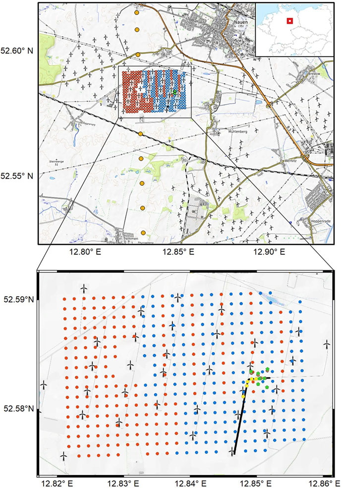
FIGURE 1. Geometry of the experiment in the wind farm near Nauen (north-eastern Germany). The 2D array is composed of 200 4.5-Hz one-component geophones (red circles) and 200 5.0-Hz three-component sensors (blue circles) positioned on a 100-m grid. In the south-eastern sector, the grid was densified by Lennartz 5-s short period sensors (yellow circles), iXblue blueSeis-3A rotational seismometers co-located with Trillium compact 120-s seismometers (green circles) and pressure sensors (brown circles). The black line represents the position of the optical fiber. The radial line array extending north-south with Trillium Compact 120-s broadband instruments is represented by orange circles.

The wind turbines are mainly identically constructed turbines of the types Wind World WW 750 with a hub height of 73.9 m and NEG Micon M1500-750 with a hub height of 73.8 m, both of them having rated output power of 750 kW. In the south-eastern sector of the seismic array, seven wind turbines are of the type ENERCON E-70 with hub heights of 113 and 114.5 m. In the transition area between these two areas there are still four wind turbines NEG Micon NM82/1500 with a hub height of 93.6 m. All types are variable-speed wind turbines, i.e., their blade rotational speed varies with incident wind speed although they all begin to operate only if the wind speed exceeds a threshold value of approximately 3 m/s.

3 Data analysis and interpretation

3.1 Spectral ratios

As a first examination of the role of the field of wind turbine towers on the seismic wavefield we calculate the ratio between the Fourier spectra (vertical component) measured separately for all sensors in the wind farm and for the three southern-most broadband station which are located far enough outside the wind farm so that it can be assumed that their recordings are not directly affected by the wind turbines. For each station, we take a 1-h signal starting at midnight on 16 February 2023 when there was almost no wind (less than 2 m/s average wind speed at the top of the wind turbines, most likely no rotation of the wind turbine blades). We divide the 1-h window into 120-s long windows, each of which is tapered with a 5-per cent cosine function. The corresponding Fourier spectra are then averaged for stations inside and outside the wind farm and the corresponding mean spectral ratio with a confidence interval as the standard deviation of all averaging processes shown in Figure 2A. As a side note, we have assured that the spectra are reliable for frequencies lower than 1 Hz since we have set the pre-amplifier gain to 8 and since the input level of noise is significantly higher than the minimum new low-noise model of Peterson (1993) in this frequency range. For comparison, Figure 2A also shows the horizontal-to-vertical spectral ratio (HVSR) for the southernmost station of the radial array. The latter (Nogoshi and Igarashi, 1970; 1971; Bard, 1999) is a passive technique that can be used to estimate a resonance frequency and a lower-bound level of amplification of the soft soil layers above the main impedance contrast.

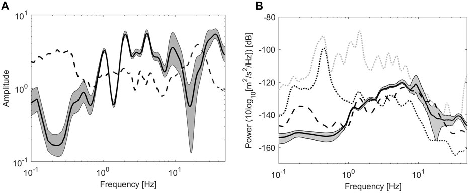
FIGURE 2. (A) Spectral ratios (vertical component) between the 400 array nodes and the three most distant broadband stations outside the wind farm (solid line plus/minus one standard deviation). The dashed line corresponds to the horizontal-to-vertical spectral ratio for the southernmost broadband station. (B) Power spectral densities of the 400 array nodes (solid line) and the broadband stations (dashed line). The dotted lines show the geometrical mean of the two horizontal components of the 5-s sensor installed on the foundation of a single wind turbine during operation (gray) and at standstill (black).

Three strong minima for the inside-to-outside spectral ratio can be identified at around 0.25, 1.4 and 13 Hz. At these frequencies, the spectral amplitude in the wind farm is smaller by a factor of more than 5 compared to the neighbouring frequencies. Other smaller minima can be seen between 3 and 4 Hz and around 8 Hz. The occurrence of these spectral minima is well constrained, in particular for intermediate frequencies, and larger standard deviations only occur for the first minimum and for frequencies higher than ∼ 7 Hz. Looking at the HVSR and comparing it with the data in the frequency domain represented by the power spectral densities (PSDs) for stations inside and outside the wind farm (Figure 2B), it can be concluded that these troughs cannot be related to soil resonance effects at the stations outside the wind farm, meaning that the spectral pattern reveals a strong attenuation of the wavefield between the individual wind turbines. In these frequency bands, the spectral amplitude inside the wind farm is reduced relative to the spectral amplitude outside and significantly less energy penetrates through the ground. The only exception to this is the peak at 0.25 Hz in Figure 2A which might be amplified due to an increased amplitude of the vertical spectra of the outside station. This could either be caused by soil resonance effects or due to secondary microseisms which the geophones were not able to record sufficiently well.

3.2 Rayleigh wave dispersion curve

If less energy is propagating through the wind farm in certain frequency ranges, this effect may also be observed in other space-frequency patterns. To estimate the dispersion curve of Rayleigh waves, we consider two different methodologies, the Extended Spatial AutoCorrelation (ESAC, Ohori et al., 2002 based on Aki, 1957) and the slant stack method, described by Thorson and Claerbout (1985). The former is based on the calculation of the spatial correlation coefficients between pairs of stations which are then fitted to Bessel functions for a range of frequencies. In this way, for each frequency, the average phase velocity can be obtained. The slant stack method translates seismogram amplitudes relative to distance and time to amplitudes relative to the ray parameter (the inverse of the apparent velocity) and an intercept time. This in turn gives a power spectral density function, which is a representation of signal strength as a function of frequency and apparent phase velocity. While the ESAC method provides reliable dispersion curves over a broader frequency range, especially toward lower frequencies, the slant stack method can determine the frequency ranges where higher surface wave modes dominate.

Here we take a total of 120 non-overlapping vertical component signal windows from all geophones, each window being 120 s long, again starting at midnight on 16 February 2023 when almost no wind prevailed and the blades of the wind turbine were not expected to have rotated. As shown in Figure 3, the two approaches provide equivalent average dispersion curves spanning a range from 0.4 to 4 Hz with phase velocities ranging from 900 to 350 m/s and corresponding wavelengths ranging from 90 m to over 2 km. As usual, the slant stack approach shows decreasing resolution for lower frequencies and cannot be used for frequencies much lower than 1 Hz. Although the dimension of the entire array should allow a determination of phase velocities at even lower frequencies, incoherent noise prevents the use of the ESAC analysis in long wavelength range (Cho and Iwata, 2021). A representation of the covariance matrix, discussed below (cf. Figure 5B), will confirm this hypothesis.

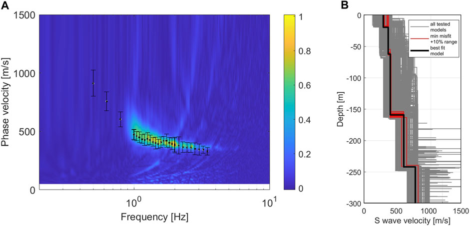
FIGURE 3. (A) ESAC (black dots) and slant stack (colour scale) Rayleigh wave dispersion curves. For the latter the colouring indicates the calculated wavefield power normalized relative to the maximum at each processing frequency. (B) S wave velocity profile showing all tested models (gray lines), the minimum cost model (black line) and all models within the minimum cost ±10% range (red lines).

Between 1 and 2 Hz, the dispersion curves from both methods are characterized by a flat shape–there is even a slight through around 1.4 Hz. As we can assume from the slant stack image, only a single mode is present. In order to check that there is no mode interference of different propagation modes that would either cross or overlap in the time-frequency space (commonly referred to as mode kissing or osculation phenomenon, Forbriger, 2003), we determine a one-dimensional S wave velocity profile by a joint inversion of Rayleigh wave dispersion curve (as shown in Figure 3) and the HVSR from the three-component sensors inside the wind farm based on Parolai et al. (2005). Herein, the dispersion curve is considered to be an apparent one (Tokimatsu et al., 1992). This approach has the advantage to properly account for all modal contributions which means that an explicit mode-number identification is not required (O’Neill and Matsuoka, 2005). As we do not observe strong lateral variations in the shape of the HVSR within the wind farm, the inversion is performed out under the assumption that the structure below the site is nearly 1D for the studied frequency range. During the inversion analysis, the S wave velocity and the thickness of the individual layers were allowed to vary within pre-defined but large ranges while the density of the soil and its P wave velocity were constrained based on geological information and the results provided of Kitsunezaki, (1990).

As shown in Figure 3, inside the wind farm, the sedimentary layers uniformly extend for several tens of meters with S wave velocities increasing steadily and ranging from 400 to just over 800 m/s. No significant impedance contrasts are mapped down to a depth of more than 300 m. This is expected as also the HVSR curves (as shown in Figure 2 for a station near the wind farm) are characterized by low amplitude levels. The narrow distribution of models with a misfit of 10% of the best-fit model around this best-fit model itself (red curves in Figure 3B) is another indication that the S wave velocity profile is well constrained. As we do not observe any large velocity contrasts and/or velocity inversions, it is reasonable to assume that the dispersion curve is representative of the fundamental mode only. The dispersion curve, however, does not show any anomalous behaviour with frequency ranges at which strong bending occurs.

3.3 Influence of infrasound signals on the seismic records

As we are dealing with data recorded in a wind farm, one has to be aware that a seismological footprint of atmospheric pressure perturbations on the recorded signals might also exist. This means that for a proper interpretation of the seismic data, in particular the spectral troughs in Figure 2A, it is necessary to investigate whether the ground motion signals might actually be caused by the pressure fluctuations or by ground vibrations. Such disturbances can also induce ground motion through the ground’s elastic response to pressure forcing. These compliance effects include both pressure disturbances arising from atmospheric dynamics and horizontally propagating infrasound waves. They were first described by the plane wave approximation by Sorrells et al. (1971) for a homogeneous half-space and by Kenda et al. (2017) for a layered soil structure. The inertial effects are much stronger for infrasound signals than for pressure perturbations moving at wind speed. The pressure forcing creates ground displacement in the horizontal and vertical directions with the horizontal motion being in phase with the pressure, whereas vertical ground motion is phase shifted by 90° relative to the pressure. Garcia et al. (2021) perform an extensive search of the seismic and pressure data for pressure infrasound signals that produce ground signals through compliance effects.

To study the compliance effects, we focus on two time periods during 14 February 2023: the early day around 06:00 UTC that present infrasound signals due to the slamming of the door of a truck deployed in the field, and the late night between 22:00 and 23:00 UTC when the wind was not blowing at the ground level but it was at the top of the wind turbine. This second time period is interesting because the noise on the pressure sensors induced by the wind is minimum whereas the blades of the wind turbines are rotating. In a first step, we process the door slam events in order to estimate the compliance from these events. The 90° phase shift between the pressure vertical velocity during such events is clearly visible in Figures 4A, B. The compliance estimate is done through envelope ratios by using narrow-band pass filtered data. Figures 4C, 4D presents the compliance values estimated in the frequency range between 0.2 and 3 Hz. The compliance values increase above 1 Hz due to a higher sensitivity to soft layers near the surface.

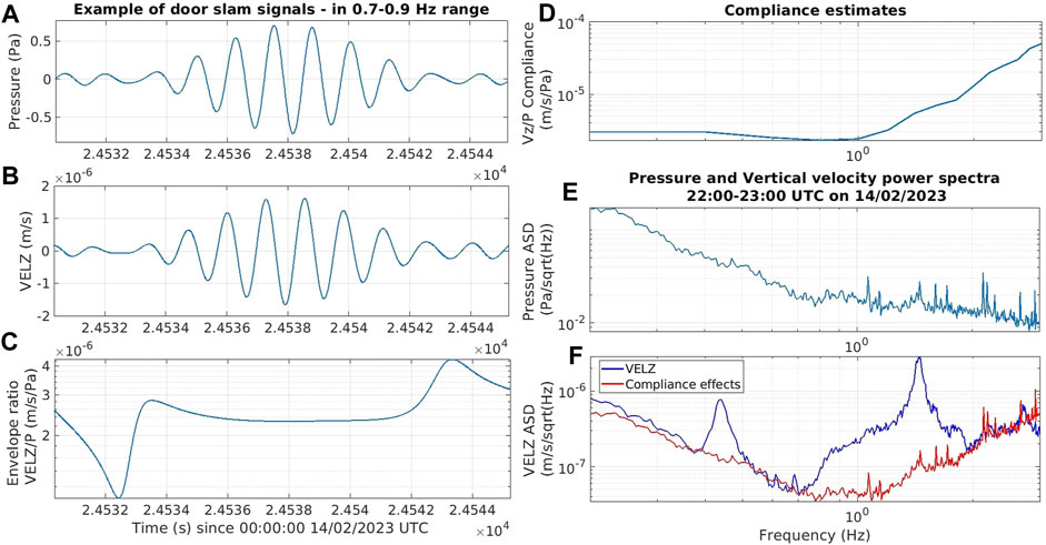
FIGURE 4. Pressure (A), vertical velocity (B) and energy envelope ratios of vertical velocity to pressure (C) filtered in the frequency range between 0.7 and 0.9 Hz range during a door slam event on 14 February 2023. On the right, compliance estimates in the frequency range between 0.2 and 3 Hz range (D) and Amplitude Spectral Density (ASD) of pressure (E) and ground velocity records (F) during the time range 22:00–23:00 UTC on 14 February. The red curve in (F) is an estimate of the vertical ground velocity variations induced by compliance effects (the product of the curves in panels (D, E).

We then use the data from the second time period to estimate how much of the signal from the seismic sensors could be attributed to compliance effects. During this period, the blades of the wind turbines are rotating and several peaks in the pressure Amplitude Spectral Density (ASD) are observed in the 0.4–3 Hz range (Figure 4E). Some of these signals can be attributed to infrasound generated by the wind turbines. Multiplying the pressure ASD by the estimated compliance values provides an estimate of the compliance effects (red curve in Figure 4F) which can be compared to the measured ASD of vertical ground motions by the co-located broadband seismometer (blue curve in Figure 4F). This comparison clearly indicates that the two main peaks around 0.43 and around 1.4 Hz are not due to compliance effects whereas the peaks in spectra of the broadband seismometer between 2.13 and 2.3 Hz are mainly driven by compliance effects. The source of these infrasound waves is probably external to the wind farm. The comparison of the ASD suggests that compliance effects are over-estimated for frequencies higher than 2.6 Hz, probably because the door slamming events have a poor signal-to-noise ratio above 2.6 Hz, thus generating a larger error in the compliance estimates in this frequency range. In contrast, the two main peaks at 0.43 and 1.4 Hz are due to causes other than pressure interference and infrasound waves.

3.4 Time-dependence of resonance effects

Of course, when studying wind turbines, an obvious question might arise to what extent the wind and the prevailing wind speed will contribute to the observed effects. A general correlation between meteorological parameters, the operation of a single or only a limited number of wind turbines and the corresponding seismic signals has already been studied by several authors (Withers et al., 1996; Zieger and Ritter, 2018; Neuffer et al., 2019; Limberger et al., 2022 among others), indicating that narrow spectral amplitude peaks can develop with increasing wind speed. From the PSDs for the station installed on the foundation of a single ENERCON E−70 wind turbine (Figure 2B), spectral peaks around 0.43, 1.4, 4 and 8 Hz can be observed both during operation at high wind speed and at standstill due to maintenance operations on 23 February between 11:00 and 12:55 UTC. This indicates that the observed peak frequencies represent tower resonance effects while additional spectral peaks during operation are expected to represent wind turbine excitation frequencies (e.g., turbine rotation, rotor blade passing) and multiples thereof.

To quantify the temporal stability of these effects over the 2-week period of the experiment, Figure 5A shows the spectrogram from continuous seismic time series. The spectrograms are calculated from the measured spectral ratios (vertical component, 120-s long windows) between the 400 stations inside and the three southernmost stations outside the wind farm. Over the entire period, the spectral shape is very stable and the spectral signatures of the wind farm dominate over much of the array, particularly at times of moderate-to-high wind speeds. As can already be seen from Figure 2, for intermediate frequencies between 1 and 10 Hz, peak amplitudes are slightly higher for increased wind speeds though the differences are less than a factor 3.

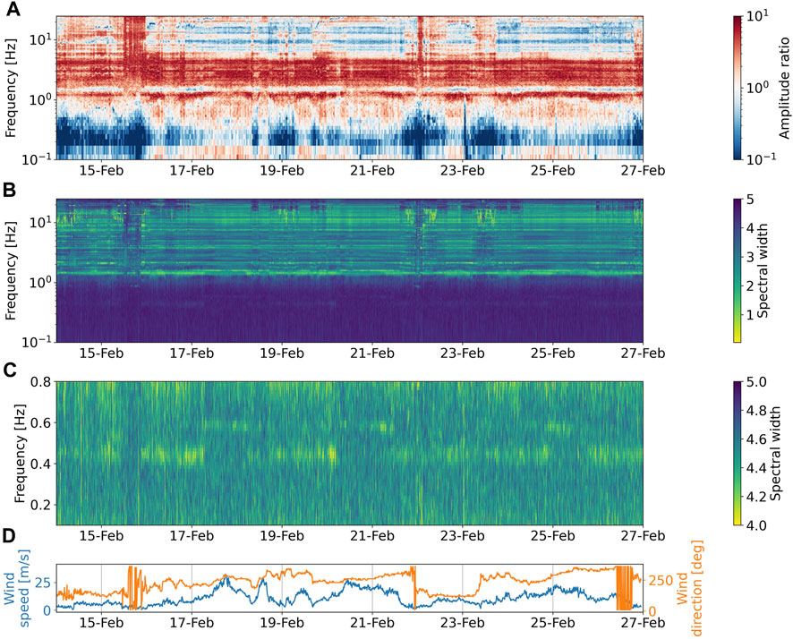
FIGURE 5. (A) Spectrogram for the spectral ratio between the array nodes and the most distant broadband stations to the south of the wind farm. (B) Spectral width of the covariance matrix of a subarray of 16 vertical component time series within the large nodal array estimating the spatial coherence of the seismic wavefield. (C) A zoom on (B) with an adapted color-scale highlighting the spectral width minimum around 0.43 Hz. (D) Wind speed and wind direction measured at the top of a wind turbine with 10-min sampling interval.

Besides building the spectral ratio, we also calculate the spectral width of the covariance matrix of the time series (vertical component) of 16 geophones inside the wind farm in the south-eastern sector (Figures 5B, C). The spectral width is a measurement for the eigenvalue distribution of the covariance matrix and reflects the spatial coherence of the seismic wavefield. A high spectral width indicates a diffusive wavefield with a low spatial coherence while a low spectral width indicates a high spatial coherence. This measurement has been introduced to identify coherent seismo-volcanic tremor signals (Seydoux et al., 2016) and has been applied to identify flexural resonances in an elastic metamaterial (Lott et al., 2020b). Due to the eigenmodes and seismic signals generated by the wind farm one might expect a rather coherent wavefield. Interestingly, the covariance matrix spectral width shows similar patterns as for the spectral ratio. There are temporarily relative stable values for the minima of the spectral width between 1 and 10 Hz, indicating a coherent wave field due to the tower resonances displayed by the greenish colors. On the other hand, as expected, a low spatial coherence can be observed for microseisms, i.e., for frequencies less than 1 Hz (e.g., Correig and Urquizú, 2002).

We further would like to point out that the large values in the spectrogram and the contemporaneous small values for the spectral width towards the end of 15 and 21 February, to a lesser extent also on 23 February, are interpreted as disturbing signals due to the rotation of the nacelle due to changing wind incidence direction as well as due to the permanent starting and stopping of the rotation of the blades. During these periods, the wavefield shows a more uncorrelated behaviour and these minima become less prominent. However, the minima at 1.4, 4 Hz and around 8 Hz appear to be more stable than the other minima (e.g., towards the end of 15 February).

This means that external factors like wind speed or blade rotation frequency will cause a variation in the amplitudes of the certain spectral peaks while the resonance frequencies of the tower eigenmodes remain stable in time. More importantly and also clearly visible in Figure 5, the spectral troughs around 1.4 and 13 Hz, to a lesser degree also at 8 Hz, at which significantly less energy is transmitted to the ground, are also temporarily stable with their amplitude being smaller than 1 for most of the time (pale and blueish horizontal lines in Figure 5A, most visible between 17 and 22 February and after 24 February). This holds both for small and high wind speeds Figure 5D and seems to confirm that the inside-to-outside spectral minima described in section 3.1 are caused by the strong interaction due to local resonances of the large number of wind turbine towers in the wind farm. As already mentioned above, the trough at 0.25 Hz might not be caused by resonance effects but this trough is likely due to the fact that the amplitude of the second microseism cannot be measured correctly due to the self-noise of the geophones in the low-frequency range while it can be assessed correctly at the broadband stations outside the wind farm.

3.5 Phase differences and signal amplitude

As there is a strong interaction between the soil and the structures, the horizontal and vertical components of the Rayleigh waves will excite the resonances of the large number of individual wind turbines around their resonance frequencies (both flexural and compressional resonances). This behaviour will induce a phase shift of π on the incoming waves, i.e., a reflection of the wavefield around the resonant frequencies of the wind turbines. When in anti-resonance, the attachment point between the earth surface and the wind turbine is at rest (Ewins, 2000; Williams et al., 2015), achieving the desired reduction of the incoming wavefield energy. Due to the sub-wavelength arrangement of the wind turbines, there is a less strong wavefield power within the wind farm between resonance and anti-resonance (smaller amplitude, i.e., greenish color in the slant stack image around 1.4 Hz, see Figure 3A) when considering the cumulative effect of the array of wind turbines.

To study the influence of possible phase differences on the amplitude decay, we calculate the phase differences between signals measured at the foundation of one wind turbine and at a single short-period station in the south-eastern sector of the seismic array. The investigated station (yellow circles in Figure 1) is located at a distance of around 50 m from the wind turbine, i.e., at the sub-wavelength scale (the wavelength for Rayleigh waves is ∼ 500 m at 1 Hz). For calculating possible phase differences, we refer to the cross-correlation analysis with a moving window with a length of 5 s and a total length of 1 hour (again starting from 16 February 2023 at midnight). The signals are filtered in narrow frequency bands around the observed minima and maxima of the inside-to-outside spectral ratio shown in Figure 2. Exemplarily, in Figure 6 we show the phase differences for frequency ranges between 0.7 and 1.1 Hz where a well-constrained peak can be seen and between 1.3 and 1.6 Hz in which the inside-to-outside spectral ratio is characterized by a strong trough. In the former case, the wind turbine and the soil are oscillating in phase as there is almost no phase difference between the signal at the foundation of the wind turbine and a station a few tens of meters away. Similar effects, although less clear, can be observed for the other frequency ranges where the inside-to-outside spectral ratio shows a trough (not shown). On the contrary, around 1.4 Hz, we observe a phase shift that is mainly limited to the range between π/2 and π, meaning that the oscillating wind turbine is mostly moving in an opposite direction at the sub-wavelength scale compared to the soil, thus decreasing its motion. This out-of-phase motion is, however, confined to the surface resonators, i.e., the wind turbines, meaning that such behaviour would not be observed for arbitrary pairs of stations in the seismic array nor when the distances between the resonators and the station approaches the wavelength of the surface waves but only on the sub-wavelength scale.

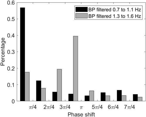
FIGURE 6. Phase shift between bandpass filtered signals at the foundation of the wind turbine with respect to recordings at a short-period station at a distance of 50 m.

In the high-frequency range, which is not affected by resonance effects, the phase differences between source signals appear rather randomly and no clear phase shift can be detected (already discussed by Saccorotti et al., 2011; Limberger et al., 2021). The scattered wavefields of the individual wind turbines lead to apparently random constructive and destructive interferences, making the interference condition very sensitive to any phase difference which can lead to strong spatial and temporal changes in the wavefield amplitude along the optical fiber (Figure 7B). In this plot, wind turbines are located at meter points 0, 350, 600 and 850 along the fiber. The respective wind turbines are located around 50, 16, 10 and 60 m away from the fiber and the blades of all wind turbines were rotating at apparently identical rotation rates at moderate wind speeds. The highest amplitude values are found for the two closest wind turbines but the corresponding amplitude pattern is not stable in time.

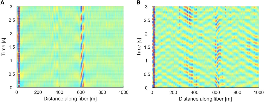
FIGURE 7. 3-s normalized strain amplitude of seismic noise along the optical fiber filtered in frequency ranges between 1.3 and 1.6 Hz (A) and 3–4 Hz (B). Measurements were taken at 16 February 2023 at 11:15 UTC. The high amplitude at very small distances is due to interfering signals due to the power supply of the interrogator.

On the contrary, a temporally stable amplitude pattern is observed in a frequency range between 1.3 and 1.6 Hz (Figure 7A). Here we see an extremely rapid drop in signal amplitude around the wind turbine resonances. Only the signals from the third wind turbine closest to the fiber at meter point 600 can be detected while for the second wind turbine at meter point 350 the signal can only be approximated (the signals from the first wind turbine are strongly disturbed by the power supply of the interrogator). After further 10–15 m, signals of the wind turbine are already barely discernible although all signals are in phase, revealing a strong damping of the wavefield inside the wind farm at the resonance frequencies of the wind turbine towers.

At first glance, it might look strange that lower frequencies of surface waves are more strongly damped. To this regard, we obtain complementary information on the attenuation by the PSD along the fiber. The PSD allows the frequency-dependent wave propagation characteristics to be revealed. After anti-alias filtering and downsampling to 100 Hz, we calculate strain-rate PSDs. We follow the procedure described by McNamara and Buland (2004) although PSDs are classically calculated for ground-motion accelerations; the relationship between ground-motion and strain-rate is not straightforward though. The PSDs calculated for each fiber channel at 16 February 2023 between 11:00 and 13:00 UTC are shown in Figure 8. PSD amplitudes strongly vary along the fiber. Signals from wind turbines at meter points 350 and 600 can clearly be identified in the high-frequency range while signals from wind turbines at meter points 0 and 850, which are around 50 and 60 m away from the fiber, are barely visible. For frequencies lower than a few Hz, only signals from the wind turbine closest to the fiber are seen. Counter-intuitively, these low-frequency signals attenuate very quickly and this effect is identical for all four wind turbines near the fiber. As wind turbines mainly emit surface waves (Styles et al., 2011 among others), intuitively one would expect stronger attenuation for higher but not for low frequencies. However, the high-frequency signals can be detected over distances of several hundred meters and it is the tower resonance frequencies that are strongly attenuated. Notably, the attenuation pattern for frequencies between 5 and 10 Hz is rather similar, already reported by Gortsas et al. (2017), with the exception that signals around 8 Hz attenuate very rapidly.

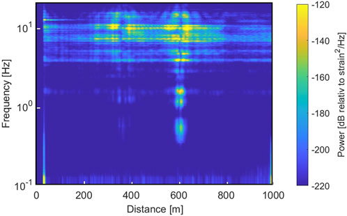
FIGURE 8. Two-hour PSDs (16 February 2023, 11:00 to 13:00 UTC) as a function of frequency and distance along the optical fiber. For a range of distances between 0 and 30 m, the signal power has been set to zero to eliminate the power supply signals from the interrogator.

3.6 Attenuation factor and attenuation length

The basic premise is that the PSD amplitude decay follows a power law, meaning that there should be a linear relationship between the logarithm of the amplitude and the logarithm of the distance. The slope of a linear fit of the decay can then be used to calculate an attenuation factor, first proposed by Stammler and Ceranna (2016) and by Flores-Estrella et al. (2017). The results in Figure 9 show peak values between 2.5 and 3 in frequency ranges around 0.43, 1.4, 4, 9 and 13 Hz. Most of these values coincide with the resonance frequencies of the wind turbine tower shown in Figure 2B. For frequencies in-between, the attenuation takes values between 1 and 2. For high frequencies above 20 Hz, there is a systematic decrease down to values between 0.5 and 1. By multiplying PSD amplitudes by a factor of 0.5, the corresponding attenuation values for time signals can be estimated as they are proportional to the square of time domain amplitudes. Note, however, that we are discussing strain-rate PSD, not ground-motion values. Nevertheless, after multiplication by 0.5, attenuation values significantly greater than 1 occur in the five distinct frequency ranges which have already been discussed earlier, indicating an attenuation even stronger than that of classical body waves, meaning that this behaviour cannot be explained by near-field effects.

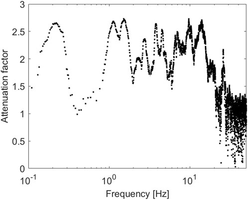
FIGURE 9. Frequency-dependent attenuation factor determined from the double-logarithmic representation of PSD amplitude decay (16 February 2023, 11:00 to 13:00 UTC).

Another way to identify the existence of frequency ranges where attenuation effects occur is to examine the correlation between different channels along the optical fiber. This involved processing of the noise data for each channel i to accumulate a coherent phase signal in the form of a cross-spectral density matrix which is the spatial covariance matrix of the data in the Fourier domain (e.g., Gerstoft and Tanimoto, 2007; Roux, 2009)

In Eq. 1, d is the Fourier transform of the data and the asterisk represents the Hermitian transpose. S is a symmetric matrix with the autocorrelations of all stations on the diagonal elements and the cross-correlations on the off-diagonal elements. As S is a function of both angular frequency ω and time t, we take a time interval of 5 s for each channel of the fiber and compute S for each angular frequency and individual time window. The results for the time-averaged cross-spectral density matrix are shown in Figure 10.

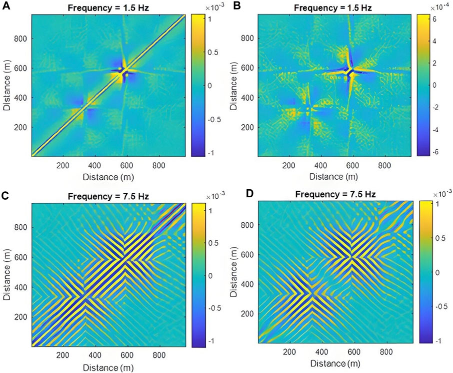
FIGURE 10. Real (A, C) and imaginary (B, D) parts of the cross-spectral density matrix along the optical fiber for frequencies of 1.5 Hz (top) and 7.5 Hz (bottom).

At 1.5 Hz the cross-spectral density amplitude drops very rapidly around the wind turbines, meaning that the scattering intensity is significant at this frequency. The coherent signal is strongly attenuated with respect to the diffusive wavefield. At 7.5 Hz the cross-spectral density amplitude remains high over a much longer distance range and a coherent signal can be detected over several hundred meters. Similar observations apply for both the real and the imaginary parts of the cross-spectral density. The latter, however, is in fact the only part of the complex cross-spectra that reflects true non-zero-lagged interactions, meaning that this observed effect does not have a time-lag with respect to the source activity of the wind turbines. A significant damping attenuation of the wave field around 1.5 Hz is also evident here while this effect cannot be observed for 7.5 Hz.

3.7 Polarization of seismic noise

In the penultimate section we discussed the phase shift of the incident waves which causes a reflection of the wavefield around the resonance frequencies of the wind turbines. Such a phase shift also exists between coupled P and SV waves, i.e., for the classical Rayleigh waves. Here the coupling between the SV waves on the vertical component and the P waves on the horizontal component is only possible if both components are shifted in phase by ±90°. Since the particle motion of the different seismic wave types is different, the key parameter for the proper identification is their polarization. The analysis is based on Vidale’s (1986) complex particle motion polarization analysis approach. A three-component ground motion recording of seismic noise is used to calculate the coherency matrix or complex covariance matrix. Kulesh et al. (2007) adapted the conventional covariance approach (e.g., Kanasewich, 1981) and utilized it to estimate time-frequency dependent polarization. In this process, time-averaging is not required explicitly. Prior to applying polarization analysis to the complex wavelet amplitude for each time-frequency pair, we first decompose the signal using a continuous wavelet transform (CWT). The ellipse, which is often inclined in 3D Euclidian space, then describes the particle motion at each time and frequency. The frequency-dependent particle motion is finally fitted to an ellipse which is characterized by its ellipticity ratio, i.e., the ratio between the minor and the major axis of the ellipse (Greenhalgh et al., 2018). The ratio takes a value of zero for a fully linearly polarized waves and a value of one for a circularly polarized arrival.

The average ellipticity ratio, i.e., the ratio of the minor to the major axis, for the seven 5-s three-component instruments inside the wind farm and the three southernmost stations outside the wind farm for 60 signal windows with a length of 120 s again starting at 16 February 2023 at midnight is shown in Figure 11. While for the latter the ellipticity ratio does not show any significant variation over the entire frequency range, for stations inside the wind farm the shape of the ellipse is frequency-dependent. For frequencies between 0.3 and 0.4 Hz, around 1.5 Hz, between 2 and 2.5 Hz and around 13 Hz there is a significant decrease towards a more linearized polarization (although the particle motion still has to be considered elliptical). These results of polarization analyses are stable in time. While, as discussed above, the trough between 2 and 2.5 Hz is likely to be caused by compliance effects (see peaks in the red curve in Figure 4F), a possible explanation for the low values in the other frequency ranges could be that the local resonances (partially) cause an energy conversion. Herein, Rayleigh waves are (partially) converted into nearly linearly polarized S waves (or more linearly polarized Rayleigh waves) at the resonance frequencies of the wind turbines in the wind farm. In the context of surface resonators over a homogeneous semi-infinite elastic medium, such conversion of the Rayleigh waves has already been predicted theoretically and observed numerically (Colombi et al., 2016a; 2017; Colquitt et al., 2017). The abrupt shift in particle motion observed in the wind farm provides a further indication of the influence of the wind turbines on the propagation of surface waves as these effects are not observed for stations outside the wind farm.

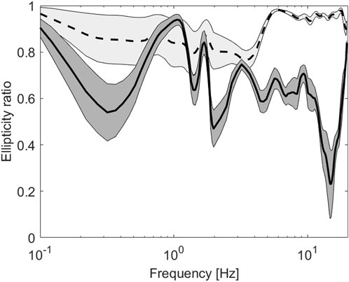
FIGURE 11. Ellipticity ratio of the reconstructed particle motion through the continuous wavelet transform for 5-s short-period stations inside (solid line) and the broadband stations outside (dashed line) the wind farm.

4 Numerical modeling of the wind turbine and discussion

Understanding the surface wave dynamics observed in this experiment also requires a good understanding of the dynamic characteristics of the wind turbine resonators present in the field. On the experimental side, there is a high degree of consistency with respect to the frequency ranges in which strong damping effects occur and some of these observations cannot be interpreted as the behaviour of individual wind turbines but only as the interaction of a large number of wind turbines. The peaks that we observe in the spectra can originate from flexural and compressional oscillations of the tower, blade rotation or power grid frequency including harmonics and subharmonics. For a numerical evaluation of mechanical resonance effects, the eigenvalues for one of the turbines in the wind farm are obtained using COMSOL Multiphysics^®, a finite element analysis program. We specifically choose to evaluate the resonances of the wind turbine from type ENERCON E-70 which has a Lennartz 5-s broadband sensor installed at its base and the DAS fiber optic cable in close proximity. This will help us better understand the recorded signals. This wind turbine with nominal power of 2.3 MW has a hub height of 113.5 m and is mounted over a prestressed concrete-steel hybrid tower (Figure 12, left panel). The diameter of the tubular tower varies from 9.3 m at the base and smoothly tapers to 2 m diameter at the very top. The bottom two-thirds of the tower is a precast concrete construction with 22 segments, each 3.8 m high with a 300 mm thick shell. The top one-third of the tower is composed of 2 structural steel segments 3 and 25 m long, having a shell thickness of 40 and 25 mm respectively. The tower is idealised as a vertical cantilever beam of multiple segments having a mean annular cross section with constant thickness. The rotor assembly, the nacelle and generator which weigh around 104 tons in total, are modeled as a concentrated mass placed on top of the beam, whereas the bottom end of the tower is assigned a fixed boundary condition. The tower is discretised with one-dimensional beam elements available with the Structural Mechanics module of COMSOL. The elastic parameters of concrete and structural steel, as seen in Figure 12, are obtained from the Euro code 2 and 3 respectively (British Standard Institution, 2004; John Wiley and Sons, 2005).

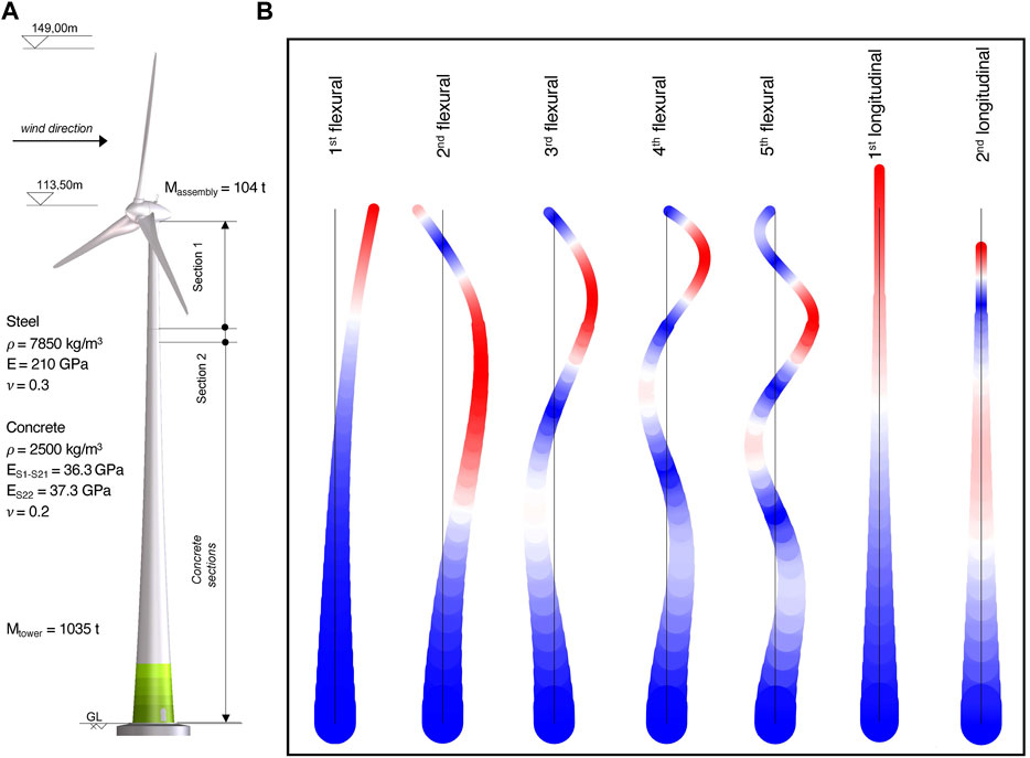
FIGURE 12. Modal representations of the 112.3 m high ENERCON E−70 wind turbine tower motion under flexural and compressional resonances. (A) Technical drawing of the wind turbine (^© ENERCON GmbH). (B) Flexural and compressional oscillations of the tower. The concrete and steel segments are assigned a uniform annulus cross section with material properties shown in the left panel. Although 1D beam elements are used, the tubular representation of the tower is shown for better visualisation. The color represents the normalized eigen displacement magnitude, blue and red indicating the respective minimum and maximum for each characteristic mode. The eigenvalues corresponding to the Euler-Bernoulli and Timoshenko beam formulations are shown in Table 1.

Table 1 lists the natural frequencies of the tower for both the Euler-Bernoulli (slender beam) and Timoshenko beam (thick beam) formulations. As can be seen from the table, the fixed-base model predicts the natural frequency of the wind turbine with reasonable accuracy. The slightly lower eigen values for the fundamental mode may be due to neglecting the steel reinforcement of the concrete sections as well as the pre-stress that would further stiffen the tower. Although our model does not take into account the flexibility of the foundation due to the soil coupling, the numerical results obtained are evidence that the foundation is almost clamped due to the type of foundation system that has been used. We do not have information on the foundation system. For soft soil sites like that in Nauen, deep foundations are usually used with micro-piles for resisting traction but it is very difficult to imagine the size, the number and the length of such piles, if any.

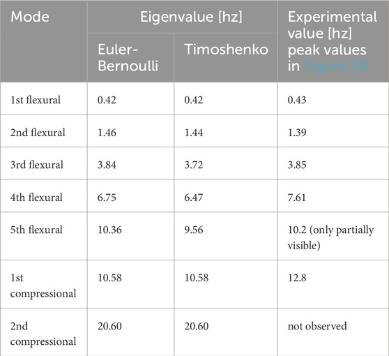
TABLE 1. Numerically obtained eigenvalues of the ENERCON E-70 wind turbine tower and comparison with the experimental results with values taken from the 5-s sensor installed on the foundation of the single wind turbine (black dotted line in Figure 2B).

The numerical modelling allows two observations to be made. First, over the whole frequency range, the eigenvalues are in good agreement with the observations and small deviations can only be seen for higher modes. Apart from the unknown foundation clamping, such deviations might also be caused by the eccentricity of the head mass with respect to the centre of gravity of the tower cross-section. This causes the resonance frequencies to widen (seen in Figure 2B when the wind turbine is operational with respect to when it is non-operational and higher modes to shift. However, since Rayleigh waves have an elliptical polarization, which implies both horizontal and vertical displacements, a straightforward coupling of both the flexural and the compressional resonances of the wind turbine towers with the seismic wavefield is also possible.

Secondly, most of the resonances here are caused by flexural modes. This might be due to the fact that flexural resonances of slender structures like wind turbines are excited more easily than compressional ones. This is different from the METAFORET experiment in which no efficient coupling between the horizontal components of the Rayleigh waves with the flexural resonances of the trees was observed which might be due to different material properties. A few theoretical studies have focused on flexural resonances and its interaction with the seismic wavefield indicating that these flexural resonances can play an important role in certain material regimes (Xiao et al., 2012; Colquitt et al., 2017; Lott and Roux, 2019; Wootton et al., 2019; Marigo et al., 2020). In particular, flexural resonances become more important for less rigid substrates (i.e., softer and more flexible soils) but that is exactly what we see in our experiment.

Although from a theoretical point of view we do not see an overlap between the flexural and compressional resonance frequency ranges, we cannot exclude the possibility of interaction between the two. However, it seems clear that for the first compressional resonance around 13 Hz, its effect on the seismic wavefield is stronger. This can be seen from the lowest troughs in Figures 2, 11 and the highest peak in Figure 9 caused by the compressional resonances of the wind turbine. Consistent with the findings of Roux et al. (2018) and Lott et al. (2020a), this may be due to the surface waves being more strongly slowed down and damped around the compressional resonance of the resonators.

While it seems clear that the set of wind turbines in the wind farm does have an impact on surface waves propagation in distinct frequency ranges, the results also indicate that there is no complete extinction of the surface wavefield as observed in classical metamaterials but only a metamaterial-approximate behaviour. Several possible factors are at play here.

(1) The frequency ranges of flexural resonances overlap with the passband of compressional waves, i.e., no compressional resonances are found below 10 Hz. Longitudinal (Rayleigh) waves can still propagate throughout the wind farm in the frequency ranges of the flexural resonances as can also be seen in Figure 11, meaning that there is no full elimination of (Rayleigh) surface waves. Similar observations have already been made by Ma et al. (2016).

(2) As we do not have a single height for all wind turbines, the damping effects associated with different heights overlap, i.e., we are mapping effective material properties. This, in turn, will cause a weakening of the overall damping but a broadening of the frequency ranges in which the damping occurs (similar to what has been described by Colombi et al., 2016b; Li and Li, 2020).

(3) Although the arrangement of the wind turbines in the north-south direction is periodic, in 3D the chosen wind farm is not sufficiently periodic for “seismic crystal” effects to become dominant as described by Colombi et al. (2016c) and by Qahtan et al. (2022).

(4) For the dispersion curve (Figure 3), we do not observe a clear slowdown of surface wave velocities around 1.5 Hz as predicted theoretically in previous studies (e.g., Colombi et al., 2016b; Colombi et al., 2017) but we only observe a flattening of the dispersion curve. This could be due to the interaction of the surface waves with body waves in the frequency range of the flexural resonances of the wind turbines.

(5) Although we see a significant influence of the wind farm on the seismic wave field in a broad frequency range, given the rather soft soil conditions (Figure 3) and a spacing between the wind turbines in the order of a few hundred meters, the wavelengths are rather short. This means that only the first two modes are really sub-wavelength (λ/8 for the first, λ/2 for the second flexural mode).

(6) In addition, the degree of coupling of Rayleigh waves and hybrid Rayleigh waves at the soil-resonator interface is sensitive to the mass of the resonator. Such heavy masses–here we are discussing masses in the order of much more than 1,000 tonnes–do not cause a smooth bending of the dispersion curve for frequencies smaller than the resonance frequencies but a very sharp deviation of the dispersion curve towards low velocities just before this frequency (Boechler et al., 2013; Palermo et al., 2016).

(7) The heavy masses are associated with a strong impedance contrast at the soil-resonator interface. Assuming values for ${\rho }_{\text{soil}}\approx$ 1800 kg/m³, ${\rho }_{\text{steel}/\text{concrete}}\approx$ 8,000 kg/m³, ${v_S}_{\text{soil}}\approx$ 500 m/s, ${v_S}_{\text{steel}/\text{concrete}}\approx$ 3,200 m/s results in an impedance contrast in the order of 30. While we generally observe an increase in the width of the damping frequency ranges for decreasing impedance contrasts, for strong impedance contrasts–as seen here–the corresponding damping frequency ranges tend to become smaller due to a weakened coupling between the ground and the resonators (Colombi et al., 2014; Joshi and Narayan, 2022).

(8) While previous reference studies have generally been performed for a homogeneous halfspace, a multi-layered soil will result in a more complex wavefield. The coupling of the wavefield with the resonators will then depend more strongly on the variation of the soil properties with depth (Chen et al., 2019) although a leakage to higher-mode surface waves which cannot be resolved with our experimental configuration (Lott et al., 2020a) as well as an interplay between flexural and compressional resonance resonances (as described, for example, by Marigo et al., 2020) might also be possible.

While so far we only have focused on Rayleigh waves, layered soils will practically also allow the study of anti-plane waves, i.e., Love waves requiring horizontal resonators (Palermo and Marzani, 2018). Although the overall results are consistent, there are a number of experimental peculiarities which can be excluded in theoretical studies but which are unavoidable in the real-world experiments. Such peculiarities can only be resolved by dense spatial sampling of the seismic wavefield.

5 Conclusion

We have demonstrated for the first time that tall structures at the city-district scale can interact with each other, with the seismic wavefield and with the atmospheric pressure field. The spatially dense installation of extended resonators can produce strong structural damping of Rayleigh waves in the frequency range of engineering interest (a few Hz). A dense grid of seismic geophones and complementary instrumentation allows the physical interpretation of the observed wavefield properties to be validated. Around the flexural and compressional resonance frequencies of the wind turbine towers, the coupling between the resonators and surface waves in the wind farm is demonstrated taking into account amplitude and phase patterns, attenuation length, spectral ratio and surface wave polarization. The damping effect in these frequency ranges is further clearly observed in the strain amplitude along the optical fiber. The spectral ratio between stations inside and outside the wind farm reveals that this attenuation results from the incoherent scattering linked to the interaction of surface waves with the wind turbines, meaning that these effects cannot be observed outside the wind farm and can only be explained by the interaction of a large number of wind turbines. The shift in particle motion ellipticity at frequencies near to the resonance of the wind turbines is another indicator of the resonance impact of the resonant structures on the propagation of Rayleigh waves which is supposed to be stronger for compressional resonances with respect to the flexural ones. With respect to metamaterial-like effects, although both types of resonances (flexural and compressional) certainly have an impact on the wavefield of seismic surface waves, we do not see evidence of a classical metamaterial with a strict bandgap in the sense of one or several frequency range(s) where the propagation of seismic surface waves is completely inhibited. The results still pave the way to potential future applications in terms of urban seismic hazard mitigation and/or earthquake engineering in urban environments. In a first step, for example, arrays of buildings could be studied with a focus on building component resonances like large concrete floors or an emphasis on designs of buildings with resonances in the frequency range of earthquake engineering. One could then ask to what extent the real urban organization with a highly heterogeneous building stock can contribute to the emergence of frequency ranges in which the seismic energy is strongly reduced.

Data availability statement

The datasets presented in this study can be found in online repositories. The names of the repository/repositories and accession number(s) can be found below: https://fdsn.org/networks/detail/XF_2023/.

Author contributions

MP: Conceptualization, Data curation, Formal Analysis, Investigation, Writing–original draft. PR: Conceptualization, Data curation, Formal Analysis, Investigation, Writing–review and editing. SM: Formal Analysis, Investigation, Software, Writing–review and editing. RG: Data curation, Formal Analysis, Investigation, Writing–review and editing. RS: Formal Analysis, Investigation, Writing–review and editing. CA: Conceptualization, Data curation, Writing–review and editing. FB: Conceptualization, Data curation, Writing–review and editing. PG: Investigation, Writing–review and editing. MO: Conceptualization, Formal Analysis, Investigation, Writing–review and editing. FC: Supervision, Writing–review and editing.

Funding

The author(s) declare financial support was received for the research, authorship, and/or publication of this article. The authors declare that financial support by the GeoForschungsZentrum Potsdam (GFZ) was received for the research, authorship, and/or publication of this article.

Acknowledgments

We are very grateful to the private land owners and the community of Nauen for hosting our instruments. We also thank our colleagues who came on the field for station deployment and maintenance (Andreas Brotzer, Andrés Olivar Castaño, Alex Dombrowsky, Reza Esfahani, Fandy Adji Fachtony, Annabel Haendel, Sebastian Heimann, Axel Jung, Frank Krueger, Lukas Lehmann, Henning Lilienkamp, Chen-Ray Lin, Karina Loviknes, Malte Metz, Sebastián Nuñez Jara, Laurens Oostwegel, Elif Tuerker, Nele Vesely, Daniel Vollmer, Ming-Suan Yen). Instruments were provided by the Geophysical Instrumental Pool Potsdam (GIPP), by the University of Potsdam, by the Ludwig Maximilian University of Munich and by ISAE-SUPAERO Toulouse. SM received funding from the URBASIS project (H2020-MSCA-ITN-2018, grant number 813137). We would also like to warmly thank Martin Drews, ENERCON GmbH for providing the information on the wind turbines. Map data copyrighted OpenStreetMap contributors and available from https://www.openstreetmap.org. The two reviewers and the associate editor Chong Xu are also thanked for their constructive comments which helped to improve the manuscript.

Conflict of interest

The authors declare that the research was conducted in the absence of any commercial or financial relationships that could be construed as a potential conflict of interest.

Publisher’s note

All claims expressed in this article are solely those of the authors and do not necessarily represent those of their affiliated organizations, or those of the publisher, the editors and the reviewers. Any product that may be evaluated in this article, or claim that may be made by its manufacturer, is not guaranteed or endorsed by the publisher.

References

Aki, K. (1957). Space and time spectra of stationary stochastic waves, with special reference to microtremors. Bull. Earthq. Res. Inst. 35, 415–456.
Albino, C., Godinho, L., Amado-Mendes, P., Alves-Costa, P., Dias-da-Costa, D., and Soares, D. (2019). 3D FEM analysis of the effect of buried phononic crystal barriers on vibration mitigation. Eng. Struct. 196, 109340. doi:10.1016/j.engstruct.2019.109340
Avilés, J., and Sánchez-Sesma, F. J. (1988). Foundation isolation from vibrations using piles as barriers. J. Eng. Mech. 114 (11), 1854–1870. doi:10.1061/(asce)0733-9399(1988)114:11(1854)
Bard, P. Y. (1999). Microtremor measurements: a tool for site effect estimation. Eff. Surf. Geol. seismic motion 3, 1251–1279.
Boechler, N., Eliason, J. K., Kumar, A., Maznev, A. A., Nelson, K. A., and Fang, N. (2013). Interaction of a contact resonance of microspheres with surface acoustic waves. Phys. Rev. Lett. 111 (3), 036103. doi:10.1103/physrevlett.111.036103
British Standard Institution (2004). Eurocode 2: design of concrete structures - Part 1-1: general rules and rules for buildings. EN 1992-1-1 (2004), 668. London: British Standard Institution, 659–668.
Brûlé, S., Javelaud, E. H., Enoch, S., and Guenneau, S. (2014). Experiments on seismic metamaterials: molding surface waves. Phys. Rev. Lett. 112 (13), 133901. doi:10.1103/physrevlett.112.133901
Castanheira-Pinto, A., Alves-Costa, P., Godinho, L., and Amado-Mendes, P. (2018). On the application of continuous buried periodic inclusions on the filtering of traffic vibrations: a numerical study. Soil Dyn. Earthq. Eng. 113, 391–405. doi:10.1016/j.soildyn.2018.06.020
Chen, Y., Qian, F., Scarpa, F., Zuo, L., and Zhuang, X. (2019). Harnessing multi-layered soil to design seismic metamaterials with ultralow frequency band gaps. Mater. Des. 175, 107813. doi:10.1016/j.matdes.2019.107813
Cho, I., and Iwata, T. (2021). Limits and benefits of the spatial autocorrelation microtremor array method due to the incoherent noise, with special reference to the analysis of long wavelength ranges. J. Geophys. Res. Solid Earth 126 (2). doi:10.1029/2020JB019850
Code, P. (2005). Eurocode 2: design of concrete structures-part 1–1: general rules and rules for buildings. London: British Standard Institution, 659–668.
Colombi, A., Ageeva, V., Smith, R. J., Clare, A., Patel, R., Clark, M., et al. (2017). Enhanced sensing and conversion of ultrasonic Rayleigh waves by elastic metasurfaces. Sci. Rep. 7 (1), 6750. doi:10.1038/s41598-017-07151-6
Colombi, A., Colquitt, D., Roux, P., Guenneau, S., and Craster, R. V. (2016a). A seismic metamaterial: the resonant metawedge. Sci. Rep. 6 (1), 27717. doi:10.1038/srep27717
Colombi, A., Guenneau, S., Roux, P., and Craster, R. V. (2016c). Transformation seismology: composite soil lenses for steering surface elastic Rayleigh waves. Sci. Rep. 6 (1), 25320. doi:10.1038/srep25320
Colombi, A., Roux, P., Guenneau, S., Guéguen, P., and Craster, R. V. (2016b). Forests as a natural seismic metamaterial: Rayleigh wave bandgaps induced by local resonances. Sci. Rep. 6 (1), 19238. doi:10.1038/srep19238
Colombi, A., Roux, P., and Rupin, M. (2014). Sub-wavelength energy trapping of elastic waves in a metamaterial. J. Acoust. Soc. Am. 136 (2), 192–198. doi:10.1121/1.4890942
Colquitt, D. J., Colombi, A., Craster, R. V., Roux, P., and Guenneau, S. R. L. (2017). Seismic metasurfaces: sub-wavelength resonators and Rayleigh wave interaction. J. Mech. Phys. Solids 99, 379–393. doi:10.1016/j.jmps.2016.12.004
COMSOL AB (2023). COMSOL Multiphysics® v. 6.0. www.comsol.com.
Correig, A. M., and Urquizú, M. (2002). Some dynamical characteristics of microseism time-series. Geophys. J. Int. 149 (3), 589–598. doi:10.1046/j.1365-246x.2002.01602.x
Dasgupta, B., Beskos, D. E., and Vardoulakis, I. G. (1990). Vibration isolation using open or filled trenches Part 2: 3-D homogeneous soil. Comput. Mech. 6 (2), 129–142. doi:10.1007/bf00350518
Dijckmans, A., Ekblad, A., Smekal, A., Degrande, G., and Lombaert, G. (2016). Efficacy of a sheet pile wall as a wave barrier for railway induced ground vibration. Soil Dyn. Earthq. Eng. 84, 55–69. doi:10.1016/j.soildyn.2016.02.001
Flores-Estrella, H., Korn, M., and Alberts, K. (2017). Analysis of the influence of wind turbine noise on seismic recordings at two wind parks in Germany. J. Geoscience Environ. Prot. 5 (5), 76–91. doi:10.4236/gep.2017.55006
Forbriger, T. (2003). Inversion of shallow-seismic wavefields: I. Wavefield transformation. Geophys. J. Int. 153 (3), 719–734. doi:10.1046/j.1365-246x.2003.01929.x
Gao, G. Y., Li, Z. Y., Qiu, C., and Yue, Z. Q. (2006). Three-dimensional analysis of rows of piles as passive barriers for ground vibration isolation. Soil Dyn. Earthq. Eng. 26 (11), 1015–1027. doi:10.1016/j.soildyn.2006.02.005
Garcia, R. F., Murdoch, N., Lorenz, R., Spiga, A., Bowman, D. C., Lognonné, P., et al. (2021). Search for infrasound signals in InSight data using coupled pressure/ground deformation methods. Bull. Seismol. Soc. Am. 111 (6), 3055–3064. doi:10.1785/0120210079
Gau, C., and Gau, C. (2011). Geologie des Arbeitsgebietes Berlin. Geostatistik in der Baugrundmodellierung: die Bedeutung des Anwenders im Modellierungsprozess, 7–17. (in German).
Gerstoft, P., and Tanimoto, T. (2007). A year of microseisms in southern California. Geophys. Res. Lett. 34 (20). doi:10.1029/2007gl031091
Gortsas, T. V., Triantafyllidis, T., Chrisopoulos, S., and Polyzos, D. (2017). Numerical modelling of micro-seismic and infrasound noise radiated by a wind turbine. Soil Dyn. Earthq. Eng. 99, 108–123. doi:10.1016/j.soildyn.2017.05.001
Greenhalgh, S., Sollberger, D., Schmelzbach, C., and Rutty, M. (2018). Single-station polarization analysis applied to seismic wavefields: a tutorial. Adv. Geophys. 59, 123–170. doi:10.1016/bs.agph.2018.09.002
Guéguen, P., Bard, P. Y., and Chávez-García, F. J. (2002). Site-city seismic interaction in Mexico city–like environments: an analytical study. Bull. Seismol. Soc. Am. 92 (2), 794–811. doi:10.1785/0120000306
Guéguen, P., Mercerat, E. D., Singaucho, J. C., Aubert, C., Barros, J. G., Bonilla, L. F., et al. (2019). METACity-quito: a semi-dense urban seismic network deployed to analyze the concept of metamaterial for the future design of seismic-proof cities. Seismol. Res. Lett. 90 (6), 2318–2326. doi:10.1785/0220190044
Guenneau, S., and Ramakrishna, S. A. (2009). Negative refractive index, perfect lenses and checkerboards: trapping and imaging effects in folded optical spaces. Comptes Rendus Phys. 10 (5), 352–378. doi:10.1016/j.crhy.2009.04.002
Huang, J., Liu, W., and Shi, Z. (2017). Surface-wave attenuation zone of layered periodic structures and feasible application in ground vibration reduction. Constr. Build. Mater. 141, 1–11. doi:10.1016/j.conbuildmat.2017.02.153
Jennings, P. C., and Kuroiwa, J. H. (1968). Vibration and soil-structure interaction tests of a nine-story reinforced concrete building. Bull. Seismol. Soc. Am. 58 (3), 891–916. doi:10.1785/bssa0580030891
John Wiley and Sons (2005). Eurocode 3: design of steel structures - Part 1-1: general rules and rules for buildings. EN 1993-1-1 (2005). Hoboken, NJ, USA: John Wiley and Sons.
Joshi, L., and Narayan, J. P. (2022). Quantification of the effects of an urban layer on Rayleigh wave characteristics and development of a meta-city. Pure Appl. Geophys. 179 (9), 3253–3277. doi:10.1007/s00024-022-03111-y
Kadic, M., Bückmann, T., Schittny, R., and Wegener, M. (2013). Metamaterials beyond electromagnetism. Rep. Prog. Phys. 76 (12), 126501. doi:10.1088/0034-4885/76/12/126501
Kadic, M., Milton, G. W., van Hecke, M., and Wegener, M. (2019). 3D metamaterials. Nat. Rev. Phys. 1 (3), 198–210. doi:10.1038/s42254-018-0018-y
Kenda, B., Lognonné, P., Spiga, A., Kawamura, T., Kedar, S., Banerdt, W. B., et al. (2017). Modeling of ground deformation and shallow surface waves generated by Martian dust devils and perspectives for near-surface structure inversion. Space Sci. Rev. 211, 501–524. doi:10.1007/s11214-017-0378-0
Kham, M., Semblat, J. F., Bard, P. Y., and Dangla, P. (2006). Seismic site–city interaction: main governing phenomena through simplified numerical models. Bull. Seismol. Soc. Am. 96 (5), 1934–1951. doi:10.1785/0120050143
Kitsunezaki, C. (1990). Estimation of P-and S-wave velocity in deep soil deposits for evaluating ground vibrations in earthquake. J. Jpn. Soc. Nat. Disaster Sci. 9, 1–17.
Kulesh, M., Diallo, M. S., Holschneider, M., Kurennaya, K., Krüger, F., Ohrnberger, M., et al. (2007). Polarization analysis in the wavelet domain based on the adaptive covariance method. Geophys. J. Int. 170 (2), 667–678. doi:10.1111/j.1365-246x.2007.03417.x
Kumar, R., Kumar, M., Chohan, J. S., and Kumar, S. (2022). Overview on metamaterial: history, types and applications. Mater. Today Proc. 56, 3016–3024. doi:10.1016/j.matpr.2021.11.423
Laghfiri, H., and Lamdouar, N. (2021). “The screening efficiency of open and infill trenches: a review,” in International Conference on Advanced Technologies for Humanity, Rabat, Morocco, November, 2021, 346–351.
Li, Y., and Li, H. (2020). Bandgap merging and widening of elastic metamaterial with heterogeneous resonator. J. Phys. D Appl. Phys. 53 (47), 475302. doi:10.1088/1361-6463/abab2b
Limberger, F., Lindenfeld, M., Deckert, H., and Rümpker, G. (2021). Seismic radiation from wind turbines: observations and analytical modeling of frequency-dependent amplitude decays. Solid earth., 12 (8), 1851–1864. doi:10.5194/se-12-1851-2021
Limberger, F., Rümpker, G., Lindenfeld, M., and Deckert, H. (2022). Development of a numerical modelling method to predict the seismic signals generated by wind farms. Sci. Rep. 12 (1), 15516. doi:10.1038/s41598-022-19799-w
Liu, Z., Zhang, X., Mao, Y., Zhu, Y. Y., Yang, Z., Chan, C. T., et al. (2000). Locally resonant sonic materials. science 289 (5485), 1734–1736. doi:10.1126/science.289.5485.1734
Lott, M., and Roux, P. (2019). Locally resonant metamaterials for plate waves: the respective role of compressional versus flexural resonances of a dense forest of vertical rods. Fundam. Appl. Acoust. Metamaterials Seismic Radio Freq. 1, 25–45.
Lott, M., Roux, P., Garambois, S., Guéguen, P., and Colombi, A. (2020a). Evidence of metamaterial physics at the geophysics scale: the METAFORET experiment. Geophys. J. Int. 220 (2), 1330–1339. doi:10.1093/gji/ggz528
Lott, M., Roux, P., Seydoux, L., Tallon, B., Pelat, A., Skipetrov, S., et al. (2020b). Localized modes on a metasurface through multiwave interactions. Phys. Rev. Mater. 4 (6), 065203. doi:10.1103/physrevmaterials.4.065203
Luco, J. E., and Contesse, L. (1973). Dynamic structure-soil-structure interaction. Bull. Seismol. Soc. Am. 63 (4), 1289–1303. doi:10.1785/bssa0630041289
Ma, G., Fu, C., Wang, G., Del Hougne, P., Christensen, J., Lai, Y., et al. (2016). Polarization bandgaps and fluid-like elasticity in fully solid elastic metamaterials. Nat. Commun. 7 (1), 13536–13538. doi:10.1038/ncomms13536
Marigo, J. J., Pham, K., Maurel, A., and Guenneau, S. (2020). Surface waves from flexural and compressional resonances of beams. https://arxiv.org/abs/2001.06304.
Mason, H. B., Trombetta, N. W., Chen, Z., Bray, J. D., Hutchinson, T. C., and Kutter, B. L. (2013). Seismic soil–foundation–structure interaction observed in geotechnical centrifuge experiments. Soil Dyn. Earthq. Eng. 48, 162–174. doi:10.1016/j.soildyn.2013.01.014
McNamara, D. E., and Buland, R. P. (2004). Ambient noise levels in the continental United States. Bull. Seismol. Soc. Am. 94 (4), 1517–1527. doi:10.1785/012003001
Miniaci, M., Krushynska, A., Bosia, F., and Pugno, N. M. (2016). Large scale mechanical metamaterials as seismic shields. New J. Phys. 18 (8), 083041. doi:10.1088/1367-2630/18/8/083041
Neuffer, T., Kremers, S., and Fritschen, R. (2019). Characterization of seismic signals induced by the operation of wind turbines in North Rhine-Westphalia (NRW), Germany. J. Seismol. 23, 1161–1177. doi:10.1007/s10950-019-09866-7
Nogoshi, M., and Igarashi, T. (1970). On the propagation characteristics of microtremor. J. Seism. Soc. Jpn. 23, 264–280. doi:10.4294/zisin1948.23.4_264
Nogoshi, M., and Igarashi, T. (1971). On the amplitude characteristics of microtremor (Part 2). J. Seism. Soc. Jpn. 24, 26–40. doi:10.4294/zisin1948.24.1_26
Ohori, M., Nobata, A., and Wakamatsu, K. (2002). A comparison of ESAC and FK methods of estimating phase velocity using arbitrarily shaped microtremor arrays. Bull. Seismol. Soc. Am. 92 (6), 2323–2332. doi:10.1785/0119980109
O’Neill, A., and Matsuoka, T. (2005). Dominant higher surface-wave modes and possible inversion pitfalls. J. Environ. Eng. Geophys. 10 (2), 185–201. doi:10.2113/jeeg10.2.185
Palermo, A., Krödel, S., Marzani, A., and Daraio, C. (2016). Engineered metabarrier as shield from seismic surface waves. Sci. Rep. 6 (1), 39356. doi:10.1038/srep39356
Palermo, A., and Marzani, A. (2018). Control of Love waves by resonant metasurfaces. Sci. Rep. 8 (1), 7234–7238. doi:10.1038/s41598-018-25503-8
Parolai, S., Picozzi, M., Richwalski, S. M., and Milkereit, C. (2005). Joint inversion of phase velocity dispersion and H/V ratio curves from seismic noise recordings using a genetic algorithm, considering higher modes. Geophys. Res. Lett. 32 (1). doi:10.1029/2004gl021115
Peterson, J. (1993). Observations and modeling of seismic background noise. Reston, VA, USA: USGS Technical Report, 1–95.
Pu, X., and Shi, Z. (2018). Surface-wave attenuation by periodic pile barriers in layered soils. Constr. Build. Mater. 180, 177–187. doi:10.1016/j.conbuildmat.2018.05.264
Pu, X., and Shi, Z. (2020). Broadband surface wave attenuation in periodic trench barriers. J. Sound Vib. 468, 115130. doi:10.1016/j.jsv.2019.115130
Qahtan, A. S., Huang, J., Amran, M., Qader, D. N., Fediuk, R., and Wael, A. D. (2022). Seismic composite metamaterial: a review. J. Compos. Sci. 6 (11), 348. doi:10.3390/jcs6110348
Roux, P. (2009). Passive seismic imaging with directive ambient noise: application to surface waves and the San Andreas Fault in Parkfield, CA. Geophys. J. Int. 179 (1), 367–373. doi:10.1111/j.1365-246x.2009.04282.x
Roux, P., Bindi, D., Boxberger, T., Colombi, A., Cotton, F., Douste-Bacque, I., et al. (2018). Toward seismic metamaterials: the METAFORET project. Seismol. Res. Lett. 89 (2A), 582–593. doi:10.1785/0220170196
Saccorotti, G., Piccinini, D., Cauchie, L., and Fiori, I. (2011). Seismic noise by wind farms: a case study from the Virgo Gravitational Wave Observatory, Italy. Bull. Seismol. Soc. Am. 101 (2), 568–578. doi:10.1785/0120100203
Schwan, L., Boutin, C., Padrón, L. A., Dietz, M. S., Bard, P. Y., and Taylor, C. (2016). Site-city interaction: theoretical, numerical and experimental crossed-analysis. Geophys. J. Int. 205 (2), 1006–1031. doi:10.1093/gji/ggw049
Seydoux, L., Shapiro, N. M., de Rosny, J., Brenguier, F., and Landès, M. (2016). Detecting seismic activity with a covariance matrix analysis of data recorded on seismic arrays. Geophys. J. Int. 204 (3), 1430–1442. doi:10.1093/gji/ggv531
Simovski, C. R. (2009). Material parameters of metamaterials (a review). Opt. Spectrosc. 107, 726–753. doi:10.1134/s0030400x09110101
Sorrells, G. G., McDonald, J. A., Der, Z. A., and Herrin, E. (1971). Earth motion caused by local atmospheric pressure changes. Geophys. J. Int. 26 (1-4), 83–98. doi:10.1111/j.1365-246x.1971.tb03384.x
Stackebrandt, W., and Manhenke, V. (2010). Atlas zur Geologie von Brandenburg, Landesamt für Bergbau. Cottbus, Germany: Geologie und Rohstoffe Brandenburg. (in German).
Stammler, K., and Ceranna, L. (2016). Influence of wind turbines on seismic records of the Gräfenberg array. Seismol. Res. Lett. 87 (5), 1075–1081. doi:10.1785/0220160049
Styles, P., Westwood, R. F., Toon, S. M., Buckingham, M. P., Marmo, B., and Carruthers, B. (2011). “Monitoring and mitigation of low frequency noise from wind turbines to protect comprehensive test ban seismic monitoring stations,” in Fourth international Meeting on wind turbine noise, Rome, Italy, April, 2011, 1–13.
Thorson, J. R., and Claerbout, J. F. (1985). Velocity-stack and slant-stack stochastic inversion. Geophysics 50 (12), 2727–2741. doi:10.1190/1.1441893
Tian, Y., Chen, S., Liu, S., and Lu, X. (2023). Influence of tall buildings on city-scale seismic response analysis: a case study of Shanghai CBD. Soil Dyn. Earthq. Eng. 173, 108063. doi:10.1016/j.soildyn.2023.108063
Tokimatsu, K., Tamura, S., and Kojima, H. (1992). Effects of multiple modes on Rayleigh wave dispersion characteristics. J. geotechnical Eng. 118 (10), 1529–1543. doi:10.1061/(asce)0733-9410(1992)118:10(1529)
Tsogka, C., and Wirgin, A. (2003). Simulation of seismic response in an idealized city. Soil Dyn. Earthq. Eng. 23 (5), 391–402. doi:10.1016/s0267-7261(03)00017-4
Turpin, J. P., Bossard, J. A., Morgan, K. L., Werner, D. H., and Werner, P. L. (2014). Reconfigurable and tunable metamaterials: a review of the theory and applications. Int. J. Antennas Propag. 2014, 1–18. doi:10.1155/2014/429837
Ungureanu, B., Guenneau, S., Achaoui, Y., Diatta, A., Farhat, M., Hutridurga, H., et al. (2019). The influence of building interactions on seismic and elastic body waves. EPJ Appl. Metamat., 6–18.
Vidale, J. E. (1986). Complex polarization analysis of particle motion. Bull. Seismol. Soc. Am. 76 (5), 1393–1405.
Weemstra, C., Snieder, R., and Boschi, L. (2015). On the estimation of attenuation from the ambient seismic field: inferences from distributions of isotropic point scatterers. Geophys. J. Int. 203 (2), 1054–1071. doi:10.1093/gji/ggv311
Wegener, M. (2013). Metamaterials beyond optics. Science 342 (6161), 939–940. doi:10.1126/science.1246545
Williams, E. G., Roux, P., Rupin, M., and Kuperman, W. A. (2015). Theory of multiresonant metamaterials for A0 lamb waves. Phys. Rev. B 91 (10), 104307. doi:10.1103/physrevb.91.104307
Wirgin, A., and Bard, P. Y. (1996). Effects of buildings on the duration and amplitude of ground motion in Mexico City. Bull. Seismol. Soc. Am. 86 (3), 914–920. doi:10.1785/bssa0860030914
Withers, M. M., Aster, R. C., Young, C. J., and Chael, E. P. (1996). High-frequency analysis of seismic background noise as a function of wind speed and shallow depth. Bull. Seismol. Soc. Am. 86 (5), 1507–1515. doi:10.1785/bssa0860051507
Wootton, P. T., Kaplunov, J., and Colquitt, D. J. (2019). An asymptotic hyperbolic–elliptic model for flexural-seismic metasurfaces. Proc. R. Soc. A 475 (2227), 20190079. doi:10.1098/rspa.2019.0079
Xiao, Y., Wen, J., and Wen, X. (2012). Flexural wave band gaps in locally resonant thin plates with periodically attached spring–mass resonators. J. Phys. D Appl. Phys. 45 (19), 195401. doi:10.1088/0022-3727/45/19/195401
Keywords: soil structure interaction, seismic metamaterials, local resonance, wind turbines, bandgaps
Citation: Pilz M, Roux P, Mohammed SA, Garcia RF, Steinmann R, Aubert C, Bernauer F, Guéguen P, Ohrnberger M and Cotton F (2024) Wind turbines as a metamaterial-like urban layer: an experimental investigation using a dense seismic array and complementary sensing technologies. Front. Earth Sci. 12:1352027. doi: 10.3389/feart.2024.1352027
Received: 07 December 2023; Accepted: 22 January 2024;
Published: 05 February 2024.
Edited by:
Chong Xu, Ministry of Emergency Management (China), ChinaReviewed by:
Keith Attenborough, The Open University, United KingdomLei Gao, Hohai University, China
Copyright © 2024 Pilz, Roux, Mohammed, Garcia, Steinmann, Aubert, Bernauer, Guéguen, Ohrnberger and Cotton. This is an open-access article distributed under the terms of the Creative Commons Attribution License (CC BY). The use, distribution or reproduction in other forums is permitted, provided the original author(s) and the copyright owner(s) are credited and that the original publication in this journal is cited, in accordance with accepted academic practice. No use, distribution or reproduction is permitted which does not comply with these terms.
*Correspondence: Marco Pilz, pilz@gfz-potsdam.de