Geodetic residual time series: A combined series by minimization of their internal noise level

1 Introduction

The Earth’s rotation is continuously changing, and this effect is observed in the magnitude of the Earth’s rotation and the orientation of its axis. Precise space-geodetic measurements may determine the different wobbles of the Earth. It has been found that the pole of the Earth’s oscillates mainly with free Chandler and 1 year periods. Most recent studies (Dobslaw et al., 2010; Chen et al., 2013; Adhikari and Ivins, 2016) concluded that some combination of hydro-atmospheric mass redistribution and relative motion of winds and ocean currents forces all polar motion changes. Since 2000, the improvement of hydro-atmospheric circulation models has ponted that the Chandler effect is mostly forced by the mass transport in Earth’s fluid layers (Gross, 2000; Brzeziński and Nastula, 2002). Mass redistribution and their movement within the superficial fluid layers of the Earth excite rotational changes, mainly at seasonal or shorter timescales (Wahr, 1983; Brzeziński et al., 2009; Dobslaw et al., 2010; Nastula et al., 2011; Chen et al., 2012; Seoane et al., 2012; Chen et al., 2013; Chen et al., 2017).

The effect of various geophysical excitations of the Earth’s variable rotation is studied by applying the principle of conservation of angular momentum between the atmosphere, ocean, and solid Earth. The effective angular momentum functions (EAMF) have been used to study angular momentum exchanges, leading to exciting polar motion (Wahr, 1983; Barnes et al., 1983; Eubanks, 1993; Aoyama and Naito, 2000; Dickman, 2003; Dobslaw et al., 2010.)

Many geophysical models of the atmosphere, oceans, and land hydrology exist, which enhance our knowledge of global dynamic processes in the Earth system. However, these models are very compound, and still, their uncertainties in the process descriptions, parametrization, and forcing exist (Güntner, 2008). Quantitative evaluation of the geophysical fluids, atmosphere, and ocean contribution to polar motion variation has been long investigated (Barnes et al., 1983; Chao and Au, 1991; Ponte, 1997; Gross et al., 2004). General remarks of these studies show that the excitation of polar motion is explained mainly by AAM and OAM. However, large parts of the observed polar motion excitations cannot be explained by the sum of modeled atmospheric and oceanic effects, concluding that other excitation mechanisms cause polar motion to excite. Significantly, the large-scale mass variations over the lands, including changes in soil moisture, snow and ice sheets, and groundwater, may play an important role in exciting remaining parts of polar motion (Chen et al., 2000; Nastula et al., 2007; Nastula et al., 2011; Seoane et al., 2011; Wińska et al., 2016; Śliwińska et al., 2019). In earlier works (Jin et al., 2010; Nastula et al., 2011; Seoane et al., 2011; Jin et al., 2012; Seoane et al., 2012; Wińska et al., 2016; Winska et al., 2017; Śliwińska and Nastula, 2019) geodetic residual time series, namely, GAO, have been computed and compared to global hydrological excitation functions of polar motion. Results of comparison of variability in the complex equatorial components of different geodetic residuals time series, χ₁+iχ₂, showing changes in the hydrological signal in polar motion concerning each other and the hydrological excitation coming from climate models, display significant discrepancies. Despite having the most significant impact on polar motion excitation, the atmosphere, ocean, and land hydrosphere cannot close the excitation budget entirely (Wińska et al., 2016; Winska et al., 2017; Śliwińska and Nastula, 2019). The correlations between geodetic residuals and hydrological signals in polar motion differ from one geophysical model to another. The geophysical effects on Earth’s rotation differ for various atmospheric, oceanic, and hydrological models chosen. Hence, complementary observations and numerical models are needed to link polar motion changes with individual processes acting on Earth’s fluid layers composed of the atmosphere, ocean, and continental hydrosphere.

Until now, no studies have shown that selecting one particular combination of AAM+OAM models has the best correlation with Earth rotation data–geodetic excitations of polar motion (Jin et al., 2012; Winska et al., 2017; Śliwińska et al., 2019; Śliwińska and Nastula, 2019). The choice to work with different AAM and OAM time series is entirely arbitrary. Only one criterion has been taken into account: the AAM model is combined with the OAM model forced consistently with operational analysis data from this AAM. It thus seems necessary to show differences between various GAO solutions and justifies using one combination of them that best correlate with the Hydrological Angular Momentum time series.

This investigation of the latest AAM and OAM series underlines that geodetic residuals vary and shows how hydrological excitation functions of polar motion explain them. The main goal of this paper is to show that using different combinations of mass and motion terms, both atmospheric and oceanic angular momentum may have a considerable influence on explaining changes in observed geodetic angular momentum caused by geophysical processes.

In recent studies, different mathematical methods were adopted to obtain improved geophysical excitations of polar motion (Gross, 2007; Brzeziński et al., 2009; Neef and Matthes, 2012; Chen et al., 2013). In Koot et al. (2006), the noise level of various AAMs were estimated and combined AAM time series, using time-dependent weights chosen so that the noise level of the combined series is minimal, were constructed. Chen et al. (2013) proposed an Least Difference Combination (LDC) method, where two model sets were developed by combining various model-based geophysical excitations. In Chen et al. (2017) LDC method was implemented to obtain improved atmospheric, oceanic, and hydrological/cryospheric angular momentum functions and excitation functions too.

In this paper, different geophysical models of the atmosphere and ocean are combined to determine the geodetic residual time series GAM-AAM-OAM (GAO, further called Res) of the Earth’s rotation. The main objectives are to evaluate different GAO time series estimates from different AAM and OAM models and to estimate their noise levels. A combined GAO time series are calculated as the weighted arithmetic mean from the six different geodetic residual time series of χ₁ and χ₂ components and compared to each other over a broadband of frequencies, from short-term to decadal time scales. We propose to determine the quality of the GAO’s time series by comparing the series with each other. To do that, we use the 3CH method. The combined hydrological-geodetic residual time series (Res Comb.) is compared to equatorial components of HAM determined from LSDM and from gravity data of satellite mission GRACE/GRACE-FO on to verify the usefulness of the 3CH method in finding the better explanation of observed geodetic angular momentum by geophysical processes.

The paper is structured as follows: in Section 2, the data and methodology used are described; individually, Section 2.1 includes a characterization of geodetic residuals (GAO) used as different combinations of mass and motion of various AAM and OAM models; Section 2.2 presents a description of effective angular momentum HAM LSDM polar motion excitations, and of GRACE/GRACE-FO data and process of calculating gravimetric excitation of PM, Section 2.3 clarifies the rule of the 3CH method and describes the way of developing the combined series of geodetic-residual excitation of PM and Section 2.4 describes the methods of time series comparison. Section 3 is split into two parts, where Section 3.1 presents the results of comparison for the overall variations of different geodetic excitations. Section 3.2 presents a comparison of geodetic residual time series concerning HAM LSDM and GRACE/GRACE-FO-based excitations for overall (Section 3.2.1), seasonal (Section 3.2.2), and non-seasonal (Section 3.2.3) oscillations. Finally, in Section 4, a discussion of the obtained results and conclusions is provided.

2 Data and methodology

2.1 Reference geodetic residual time series

This study comprehensively analyzes daily PM components’ daily oscillations using accurately measured PM time series and geophysical excitations computed from atmospheric and oceanic models between 2002 and 2020. Specifically, the different models and combinations of AAM and OAM mass and motion terms are tested here to confirm broadband oscillations in hydrological signal in PM being a difference between observed geodetic excitations (Geodetic Angular Momentum) and a sum of atmospheric angular momentum, AAM due to pressure changes (mass) and winds (motion), and oceanic angular momentum, OAM representations of ocean-bottom pressure (mass) and currents (motion), called GAO:

The Earth Orientation Center of the International Earth Rotation and Reference System Service (IERS) produces time series of GAM with 1-day sampling calculated from the Earth orientation parameters (EOP), referred to as IERS EOP C04 ((Bizouard et al., 2019)). These series result from a combination of operational EOP series derived from space geodetic techniques: Very Long Baseline Interferometry (VLBI), Global Navigation Satellite System (GNSS), Satellite Laser Ranging (SLR), and Doppler Orbitography by Radiopositioning Integrated on Satellite (DORIS). GAM retains consistency with the International Terrestrial Reference Frame (ITRF 2014, (Bizouard et al., 2019)) and implements the latest IAU 2006/200A precession-nutation model. Here, daily series of GAM, based on xp and yp pole coordinates from the EOP 14 C04 solution (Bizouard, 2020) was obtained from the IERS, Earth Orientation Center (https://hpiers.obspm.fr/eop-pc/index.php, accessed on 1 December 2022).

Residual time series, GAO, is computed by removing atmospheric (AAM) and oceanic (OAM) contributions from the GAM time series, which are the most accurate and stable compared to geophysical angular momentum time series coming from models and meteorological observations. The differences in GAO indicate the hydrological signals in the geodetic excitation, which may be explained by HAM computed from global land hydrological models or gravimetric observations from GRACE/GRACE-FO satellite mission.

Several versions of mass and motion terms of the atmospheric and oceanic equatorial angular momentum time series (AAM and OAM) calculated based on global circulation models are used in this study to determine the GAO hydrological signals in geodetic excitations.

Geophysical equatorial excitations of polar motion based on the AAM model were computed from the National Centre for Environmental Prediction/National Centre for Atmospheric Research (NCEP/NCAR) re-analysis model (Kalnay et al., 1996), provided by the Special Bureau for the Atmosphere of the Global Geophysical Fluids Center (GGFC) (Salstein et al., 1993). The temporal coverage of the NCEP/NCAR re-analysis model is given as four times, daily and monthly values for 1948/01/01 to present (Kalnay et al., 1996). The following components are distinguished in the AAM NCEP/NCAR time series: a pressure term (χ^p) with IB correction term due to air mass redistribution and a wind term (χ^w) due to atmospheric relative angular momentum (Zhou et al., 2006). These equatorial AAM time series are given in a sampling period of 6 h. The AAM NCEP/NCAR time series were received from the IERS Special Bureau for the atmosphere website (files.aer.com/aerweb/AAM (accessed on 29 September 2022)).

Geophysical polar motion excitations based on the ocean model include contributions from ocean currents and ocean bottom pressure variations (Jin et al., 2010). Daily values of ocean bottom pressure and ocean currents are derived from the version kf080 of the Estimating the Circulation and Climate of the Ocean (ECCO) model run at the Jet Propulsion Laboratory (Fukumori et al., 1999). The baroclinic ECCO model is forced by atmospheric surface wind stresses, temperatures, and freshwater fluxes taken from the output fields of the NCEP/NCAR reanalysis. Daily values of equatorial OAM ECCO kf080 time series are available from the IERS Special Bureau for the Oceans (https://www.ecco-group.org/geodetic-variables.htm, accessed on 29 September 2022) and cover the period from January 1993 to August 2020 (Gross et al., 2004).

A homogeneous set of geophysical excitations (AAM, OAM, and HAM) provided by the Earth System Modeling group at GeoForschungsZentrum (ESMGFZ) were included in this study. As a result of mass redistribution and the atmosphere’s relative motion, the EAMF represents the non-tidal geophysical excitations of the Earth’s orientation changes (Dobslaw and Dill, 2018). The temporal resolution of the ESMGFZ AAM has a 3 h period with 0.5⁰ grid points. To retain the non-tidal signal only in, tidal variations are extracted from the AAM data by fitting the 12 most relevant frequencies (Yu et al., 2021). Daily updated ESMGFZ AAM functions are calculated from 3h ECMWF operational analysis wind and surface pressure (http://rz-vm115.gfz-potsdam.de:8080/repository, accessed on 29 September 2022). Atmospheric surface pressure tides are subtracted from the data, and the inverted barometer (IB) correction over the ocean is applied (Dill and Dobslaw, 2019). The second source of effective angular momentum function is calculated from the ocean bottom pressures and ocean currents of an unaffected simulation by the Max-Planck-Institute from the Meteorology Ocean Model (MPIOM; (Jungclaus et al., 2013)). The OAM MPIOM ocean model is calculated with 3 h ECMWF model forces, also used for ESMGFZ AAM determination. In these OAM time series determinations, the IB correction was applied to ocean bottom pressures. The oceanic response to atmospheric tides was also estimated and removed from both mass and motion terms. Daily updated OAM time series are available from ESMGFZ from 1976-01-01 until now (http://rz-vm115.gfz-potsdam.de:8080/repository, accessed on 29 September 2022).

Seven geodetic residual time series, Res1, Res2, Res3, Res4, Res5, Res6, and Res Comb., were formed by combining different mass and motion terms of atmospherical and oceanic models from geophysical excitations (see Table 1). Note that the last solution of geodetic residuals, Res Comb., combines all six residual time series, from Res1 to Res6, computed by the 3CH method.

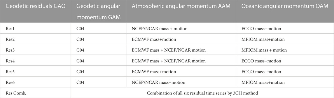
TABLE 1. GAO (Res) geodetic residual time series models based.

2.2 Hydrological angular momentum

To check the usefulness of the 3CH method in combining a solution of different geodetic residuals GAO, three different PM hydrological excitation functions, one based on the climate model and two based on GRACE-FO solutions, were provided and compared with geodetic residuals excitation functions.

The HAM time series based on the Land Surface Discharge Model (LSDM) is used in this study for comparisons. These HAM excitations are calculated from terrestrial water storage changes and capture continental water mass transport processes and storage compartments, including soil moisture, snow, rivers, lakes, runoff, and drainage channels given daily on a 0.5⁰ regular global grid (Dobslaw and Dill, 2018). Physics and parametrization of the LSDM model are based on the hydrological discharge model (HDM; (Hagemann and Gates, 2001)) and Simplified Land Surface Schemes (SLS; (Hagemann and Gates, 2003)). Additionally, the effect of barystatic sea-level changes (Sea-Level Angular Momentum, SLAM) was added to the HAM LSDM hydrological excitations. This effect causes stabilization of the sum of all masses in all three geophysical effective angular momentum components of AAM, OAM, and HAM. Hence, better consistency between observed geodetic angular momentum and geophysical excitations calculated for the combinations of AAM ECMWF, OAM MPIOM, and HAM LSDM models is expected.

The second data set comes from the Gravity Recovery and Climate Experiment (GRACE) satellite mission. Equatorial components, χ₁ and χ₂, of gravimetric-based polar motion excitations are proportional to the degree-2 order-1 Stokes coefficients of the gravity field (ΔC₂₁, ΔS₂₁) and can be calculated through (Gross, 2016),

where R = 6378136.6 m, and M = 5.9737 × 10²⁴ kg are the Earth’s mean radius and mass, respectively, and C = 8.036481 × 10³⁷ kg ⋅ m² is an axial principal inertia moment, whereas A′ = 8.010171 × 10³⁷ is a mean equatorial principal inertia moment (Chen and Shen, 2010). The factor 1.608 (Gross, 2007) takes into account the effects of the Earth’s surface loading and rotational deformation, the passive response of equilibrium to changes in rotation, and the relative angular momentum of the core caused by the changes in rotation (Cheng et al., 2011).

Eq. (2) were applied to compute χ₁, χ₂ equatorial components of the gravimetric excitations of polar motion from the newest available realizations of the operational combined monthly gravity fields of the GRACE and GRACE-FO satellite mission in spherical harmonic representation (Level-2 product) generated by the Combination Service for Time-variable Gravity Fields (COST-G; (Jäggi et al., 2023)) under the umbrella of the International Association of Geodesy (IAG). The following single solutions are included in the combined COST-G solution: AIUB RL02 and AIUB-GRACE-FO_op data, provided by Astronomical Institute University Bern, Bern, Switzerland; GFZ RL06 solution provided by GeoForschungsZentrum, Potsdam, Germany; CNES/GRGS RL05 solution provided by the Centre National d’Etudes Spatiales (CNES)/Groupe de Recherche de Géodésie Spatiale (GRGS), Toulouse, France; ITSG-Grace2018 and ITSG-Grace_op solution, provided by Institute of Geodesy at the Graz University of Technology, Graz, Austria; LUH-Grace2018 and LUH-GRACE-FO-2020 solution, provided by Leibniz Universität Hannover, Hannover, Germany; CSR RL06 solution, provided by Center for Space Research, Austin, United States of America; JPL RL06 solution provided by Jet Propulsion Laboratory, Pasadena, United States of America.

The publicly available GRACE monthly gravity field coefficients are disseminated via International Center for Global Earth Models (ICGEM) (Ince et al., 2019). Except helping the user with the choice of deciding which time series of single monthly gravity field solutions to use, combined COST-G time series represent gravity fields with reduced systematic errors (Jean et al., 2018); hence they can get better results in explaining observed polar motion excitations than single solutions from the GRACE satellite mission (Śliwińska et al., 2022).

Additionally, a single GRACE CSR RL06 solution is used to compare different combinations of geodetic residuals with the hydrological signal in exciting polar motion changes. This GRACE/GRACE-FO Level-3 data are desribed in details in work Wińska. (2022).

A 1-year gap (June 2017–June 2018) between the hydrological excitation time series computed from GRACE and GRACE-FO data was reconstructed by performance forecasting using the seasonal Autoregressive integrated moving average (ARIMA) method. To do that, the Arima function available in Matlab was used.

2.3 Three-cornered hat method–a generalized approach

The Three-Cornered Hat (3CH) method estimates the relative uncertainties of the geodetic residuals of polar motion excitation time series on the assumption that the reference dataset’s errors are unknown. This method postulates that at least three sources of time series showing the same process are needed. This method was established by Grubbs. (1948) to estimate the errors of three different instruments. 3CH method was also expanded by Gray and Allan. (1974) and was originally used to estimate oscillators’ and clocks’ stability. 3CH method has become significant in the evaluation of uncertainty in Earth orientation parameters measurements and geophysical excitation functions of polar motion and length of the day as well (Chin et al., 2005; Koot et al., 2006; Chen and Wilson, 2008; Yan et al., 2015; Ferreira et al., 2016; Meyrath and van Dam, 2016; Chen et al., 2017).

Up to now, no stochastic modeling of the noise level of different geophysical excitations computed from different AAM, OAM, and HAM models, has been made. In the 3CH method, the internal noise level of the considered time series is estimated by comparing them against each other. The 3CH method gives information about the noise without making any assumptions about the signal statistics. However, the 3CH method, in its classical formulation, hypothesizes that there is no correlation between the time series noise, which can cause inconsequential results. Here the correlations between time series were taken into account using a generalized formulation of the 3CH method. This generalization was first proposed by Tavella and Premoli. (1994) and Galindo and Palacio. (2003).

Here, we consider the geodetic residual time series stored as ${\{X_i\}}_{i=\mathrm{1,2},\dots ,N}$, where i corresponds to each solution of geodetic residual time series (N = 6). From a mathematical point of view, the 3CH method divide each solution into two terms:

where S represents a true signal, equal for all of the time series, and ϵ_i is a noise staying in the geodetic residual time series, various for each time series. The information about the noise level of each geodetic time series is calculated by performing subtraction between one reference time series and others.

In the case of the GAO time series used in this study, their noise is due to the discrepancies in modeling the atmospheric and oceanic angular momentum from one meteorological center to the other. Although each AAM and OAM time series are determined independently, the GAO time series can not be considered uncorrelated because the AAM and OAM models used the same dynamical equations and the exact data for their assimilation. Anyhow, we do not know how much the GAO time series’ noises correlate.

The generalized 3CH method has been developed by Tavella and Premoli. (1994), where the assumption of zero correlations between considered time series has not been made. The key features of this method are presented below.

Firstly, a difference between each geodetic residual time series and one of them (Res5), arbitrarily chosen as a reference, is calculated:

where X^N is a geodetic residual reference time series (Res5). Then, the patterns of the N − 1 results of the length equal to M, are integrated in an M × (N − 1) matrix as:

The covariance matrix S of the geodetic residual time series of their differences is calculated as:

Subsequently, the N × N Allan covariance matrix of the individual noises R is received. The elements of this matrix, the unknowns of the problem, will be calculated by connection to S as:

where I is the identity matrix, u is the [111 … 1]^T vector, r is the (N − 1) vector of ${[r_{1N}{r}_{2N}\dots r_{N-1,N}]}^T$ classifying the covariance estimates that involve the N’th geodetic residual time series, and r_NN is the variance of the N’th reference time series. In agreement with the Kuhn-Tücker theorem, the N free parameters of Equation 7 are separated by the minimization of the global correlation among the noises of the individual time series using an objective function:

With a constraint function ((Galindo and Palacio, 2003)):

The initial conditions were chosen to implement that the initial values gained the constraints (Torcaso et al., 2000):

When the free parameters (r_iN) have been calculated, the remaining unknown elements of $\widehat{R}$ matrix are computed subsequently using following formulae:

It is assumed that the noise level of each geodetic residual time series may vary significantly. The best representation of the differences between observed geodetic excitations and atmospheric and oceanic models as a combination of the six GAO time series compared to each other is expected in this study. A combination of the GAO time series is made by the 3CH method on the assumption that the combined time series has a noise level as low as possible.

After the noise level of each geodetic-hydrological time series was found, the combined GAO, Res. Comb., time series were computed by a combination of the six existing ones:

where the w_i(t) is the weight related to the ${\chi }_1^i$ and ${\chi }_2^i$ equatorial components of polar motion and reflecting its quality. The requirement of minimal noise variance for the combined geodetic residual time series allows determining the following normalized weights for each time series:

With the use of the 3CH method, combined geodetic residual time series (Res Comb.) of the χ₁ and χ₂ equatorial components were developed as the weighted arithmetic mean, with weights associated with the level of the variance of the noise level (Eq. (13)) calculated for each considered geodetic residuals (from Res1 to Res6). The results of weights and Res Comb. time series obtained are presented in Section 3.1.1.

2.4 Time series comparison methods

Equatorial geodetic residual time series of χ₁ and χ₂ components were compared using different methods. First, 1-day sampling geodetic residuals (from Res1 to Res6) were calculated in the 2000.00-2020.20 period. Then, Gaussian smoothing with the FWHM=30 days was applied to the geodetic residual time series. Next, long-term changes, i.e., those whose spectrum shows oscillations above 10 years, were retrieved and removed from each time series using Multi-singular spectrum analysis (MSSA method) (Wińska, 2022). Based on that processed time series, Res Comb. of χ₁ and χ₂ equatorial components were determined by the 3CH method.

Subsequently, the model, including the second-order polynomial and a sum of complex sinusoids with periods 365.25, 180.0, and 120.0 days was fitted to the geodetic residual time series. The seasonal amplitudes and phases of prograde, counterclockwise, positive frequency, and retrograde, clockwise, with negative frequency, oscillations were compared. After removing seasonality from detrended time series, non-seasonal oscillations were compared too.

Additionally, in the second part of the comparison analysis, geodetic residual time series were selected and correlated with hydrological signal in polar motion calculated from HAM LSDM hydrological model and GRACE CSR RL06 and GRACE COST-G gravimetric satellite data. Regarding that, two basic Res1 and Res2 geodetic residual time series and Res Comb. solutions were chosen as they contain all AAM and OAM considered models. In this part, geodetic and hydrological time series were interpolated monthly from 2002.3–2020.20.

The analysis was extended to Taylor diagrams, where the values of standard deviation (STD), zero-lag correlation coefficients (CORR), and root mean square differences (RMSD) of considered time series are compared (Taylor, 2001).

3 Results

The purpose of the study was to demonstrate that differences between various geodetic residual time series (Res1, to Res6, and Res Comb.), resulting from different combinations of mass and motion AAM and OAM terms, exist. These differences may impact the agreement between observed geodetic excitation of polar motion and geophysical excitations defined here as joined effects of atmosphere, ocean, and hydrology mass exchanges. In this study, Res Comb. excitations were compared with other geodetic residual time series and with GRACE/GRACE-FO based and HAM LSDM excitations. In this way utility of such a solution based on the 3CH method was tested in terms of improving the so-called geodetic budget.

3.1 Geodetic residual time series GAO

3.1.1 Overall analysis

In this section, different geodetic residual time series GAO of equatorial components, χ₁ + i χ₂, are compared to each other in terms of their long-term oscillations and overall variability. For the study of the time series of different daily GAO, the period 2000.0-2020.20 was chosen.

Figure 1 compare six different geodetic residual time series of equatorial components of χ₁ and χ₂ computed after removing mass and motion terms of different AAM and OAM models from observed geodetic excitations GAM. The analysis is done and showed over the period 2000.0-2020.2 for overall oscillations (Figure 1A), and non-linear trends comparison retrieved by MSSA method (Figure 1B).

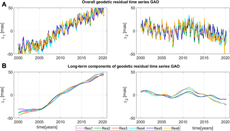
FIGURE 1. Time series of χ₁ and χ₂ equatorial components of overall (A) and long-term oscillations (B) of geodetic residuals computed from different combinations of mass and motion terms of AAM and OAM models (Res1, Res2, Res3, Res4, Res5, Res6). Long-term oscillations was computed using MSSA method for the signals reconstruction with oscillations bigger than 10 years.

In Figure 1A, strong seasonal oscillations are visible and long-term trends as well. Small differences in different geodetic residuals of polar motion in amplitudes, as well as their periodic character, are seen.

All compared geodetic residual time series show a prominent long-term trend, stronger in χ₁ and weaker in χ₂ component. These long-term changes involve global hydrological and cryospheric forces and are modified by a core-mantle coupling (Adhikari et al., 2018). Glacial Isostatic Adjustment (GIA) and surface mass load changes connected with contemporary climate, including ice sheet melting, terrestrial water storage changes, and associated sea-level variation, are potent contributors to this long-term trend (Adhikari et al., 2018). The results shown in this research are conistent by numerous studies of hydrographic and cryospheric mass changes that are equivalent to the time span of this study (Adhikari and Ivins, 2016; Chen et al., 2021).

Different geodetic residual time series are in quite good agreement in the case of their amplitudes and phases, both in χ₁, and χ₂, despite this significant differences between them occur (Figure 1A) and will be analyzed in this study. The long-term trend (Figure 1B) for each geodetic residual is similar but clearly separated by MPIOM and ECCO oceanic models, especially in χ₂.

Combined geodetic residuals, Res Com., were calculated based on geodetic residuals, from Res1 to Res2, after removing long-term changes from overall geodetic-residuals. Table 2 presents the weights computed for each geodetic residuals time series with reference solution of Res5 used for computation of the weights. As demonstrated by Tavella and Premoli (1994), the results of the 3CH method are independent of the choice of one reference series or another. The noise variance of a geodetic residual time series indicates its quality because it reflects the noise level of the series. Thus, the results can be interpreted in terms of quality: a high-quality time series will have a low noise level variance (Śliwińska et al., 2022). Non-etheless, the 3CH method, and any statistical methods, used do not allow an estimation of the absolute noise level, especially of one series. The estimated noise levels are relative, and they have no physical meaning. In general, the highest weight was assigned to the geodetic residual time series calculated from the same, as a reference value, ocean model (ECCO). In contrast, the lowest weights were received for reference geodetic residual time series (Res5) and geodetic residuals calculated from the MPIOM ocean model. It turns out that the use of different combinations of mass and motion terms derived from different AAM models does not strongly affect the agreement between observed geodetic angular momentum excitation and geophysical ones. This results from a better agreement between mass and motion terms of NCEP/NCAR and ECMWF atmospheric-based excitations than oceanic ones (Göttl et al., 2015).

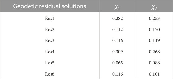
TABLE 2. Weights for six different geodetic residual time series determined with the 3CH method.

Figure 2 compares detrended geodetic residual time series of χ₁ and χ₂ components of polar motion computed as differences between overall oscillations and long-term trend variations. Here, the time series of combined geodetic residuals (Res Comb.) computed using the 3CH method are also shown. These residuals agree, especially in the χ₁ component. In the case of the χ₂ detrended oscillations, Res2, Res3, and Res6, time series differ from Res1, Res4, Res5, and Res Comb. This contrast is caused by differences in OAM ECCO and OAM MPIOM oceanic models used to calculate geodetic residuals and influence agreement between geodetic residuals time series. Geodetic residuals, Res Comb., being a combination of six existing ones, computed by minimization of their noise level by the 3CH method, is a weighted average that may improve agreement between observed geodetic signal with geophysical ones. As a result of atmospheric and land water mass changes over the Eurasian and North American continents, the χ₂ component is defined by generally higher amplitudes than χ₁. This is clarified by the higher impact on land water mass variability on this component due to the spatial distribution of the leading continents in the northern hemisphere (Chen et al., 2012).

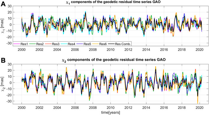
FIGURE 2. Time series of detrended χ₁ (A) and χ₂ (B) equatorial components of geodetic residuals (Res1, Res2, Res3, Res4, Res5, Res6, Res Comb.). Long-term oscillations, shown on Figure 1 were removed from original geodetic residuals GAO.

The first outcome of the evaluation of geodetic residual excitation time series calculated from different AAM and OAM solutions is displayed in Figure 3, where a time series comparison is presented in the form of Taylor diagrams. The standard deviation values, zero-lag correlation coefficients, and root mean square differences are shown simultaneously and help interpret how closely a pattern of geodetic residual excitation series matches to reference value, chosen here as geodetic residual time series calculated from AAM NCEP/NCAR and OAM ECCO models (Res1).

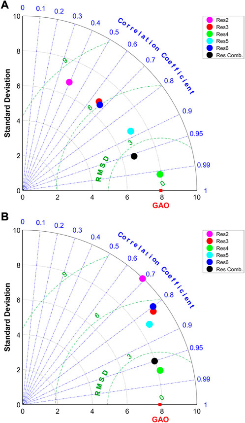
FIGURE 3. Taylor Diagrams showing a comparison of χ₁ (upper panel (A)), and χ₂ (bottom panel (B)) components of different geodetic residuals (GAO=Res1, as referenced value). The comparison is done for time series presented in Figure 2.

It can be seen that the dispersion of the geodetic residual time series obtained from different combinations of AAM and OAM models is high. The correlation coefficient values range from 0.39 (Res2) to 0.99 (Res4) for χ₁ and from 0.68 (Res2) to 0.97 (Res4) for χ₂, wherein the Res Comb. solution is very close to that one obtained from ECMWF_mass + NCEP/NCAR_motion and ECCO_mass+motion models (Res4). RMSD values are between 1.0 (Res4) and 8.1 mas (Res2) for χ₁ and between 2.4 (Res4) and 5.8 mas (Res3) for χ₂, while standard deviation values are as high as 7.9 (Res4) to 6.8 (Res2) mas for χ₁ and 7.7 (Res4) to 9.1 (Res3) mas for χ₂. The analysis of standard deviation values displays that depending on the combinations of different AAM and OAM models exploited, geodetic residuals excitation series underestimate the variability observed for the referenced value of Res1 in χ₁ component and overestimate geodetic residuals Res1 in χ₂ component. It can be seen that Res4 time series are characterized by the highest consistency with referenced value Res1. However, it should be remembered that the Res4 solution has been processed as a combination of ECMWF_mass + NCEP/NCAR_motion and ECCO_mass+motion models and in contrast to Res1 differ by AAM mass term only.

3.2 Geodetic residuals vs. hydrological angular momentum

3.2.1 Overall comparison

A comparison of selected geodetic residual time series between hydrological excitations of polar motion was conducted for further studies. To do that, three geodetic residuals were chosen, Res1 based on NCEP/NCAR and ECCO models, Res2 based on ECMWF+MPIOM models, and Res Comb. being weighted arithmetic mean of six time series considered in previous Section 3.1.1. The mass and motion terms of effective angular momentum functions due to mass transport processes in the atmosphere (ECMWF-GFZ model), the ocean (MPIOM-GFZ model), and the continental hydrosphere (HAM GFZ model) are consistent between themselves. This means that the sum of all masses in the atmosphere, ocean, and continental hydrosphere is constant (Dobslaw et al., 2010). Similarly, NCEP/NCAR is an atmospheric forcing data set for associated ECCO ocean models (Yu et al. (2021)), but these AAM and OAM models are associated neither with HAM LSDM or GRACE solutions.

Geodetic residual time series, HAM LSDM-based, GRACE CSR, and COST-G excitations were interpolated to the time of chosen HAM-based COST-G gravimetric time series.

In Figure 4, overall components (a), their long-term changes (b), as well as detrended values (c) are shown for the common period 2002.2 to 2020.0. Long-term variability was computed using the MSSA method (L=72 months window size). The strong seasonal signal is present in all geophysical time series, both in the χ₁ and χ₂ components. Overall components of different geodetic residuals and HAM LSDM and HAM-based COST-G gravimetric excitations differ. The long-term trend, the effect of GIA and climate changes, is marginal positive in χ₁ HAM LSDM, which is in line with previous work (Dill, 2008). The long-term trend of the COST-G solution is in agreement with all considered geodetic residuals in the case of χ₁ component but differs from geodetic residuals and HAM LSDM in the case of χ₂. These differences between GRACE/GRACE Follow-on and GAO long-term trends may be related to the implementation and interpretation of the pole tide correction in GRACE/GRACE-FO data processing (Chen et al., 2021). Changes in Terrestrial Water Storage (TWS) and global cryosphere explain nearly the PM amplitude and mean directional shift. In contrast, atmosphere and ocean mass added only slightly improved this agreement (Adhikari and Ivins, 2016). It suggests that GAO geodetic residuals time series do not fully explain the long-term trend and do not fully represent the global-scale continent-ocean mass transport integrally.

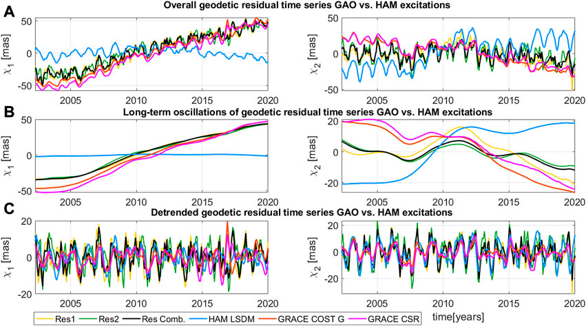
FIGURE 4. Time series comparison of equatorial components of the χ₁ and χ₂ of geodetic residuals (Res1, Res2, and Res Comb.) and gravimetric-based excitation determined from GRACE/GRACE-FO solution of CSR and COST-G solutions and HAM LSDM excitaions for (A) overall, (B) long-term trend, and (C) detrended oscillations. The non-linear long-term oscillations were deremined using MSSA method.

Further analysis of the comparison between geodetic residuals and hydrological angular momentum functions will be performed on detrended time series after removing long-term variations from overall oscillations.

From visual inspection of detrended time series (Figure 4C), some discrepancies between time series exist, both in the χ₁ and χ₂ component. The highest amplitudes are present for the Res1 in χ₁ and Res2 in χ₂ component of geodetic residuals, while the signal computed from solutions of various GRACE data and HAM LDSM model is smaller than geodetic residuals. Compatibility between all geophysical time series is pretty good, especially in the χ₂ component, but still far from perfect.

These detrended time series were compared in terms of their correlation coefficients, standard deviations, and RMSD displayed on the Figure 5 with various reference time series:(a) χ₁ of Res Comb. (b) χ₂ of Res Comb., (c) χ₁ of Res1, (d) χ₂ of Res1, (e) χ₁ of Res2, (f) χ₂ of Res2. This way, the influence on agreement between various geodetic residuals and geophysical models is shown.

From Figures 5A, B, with the reference value of combined Res Comb. solution, it can be concluded that in contrast to geodetic residuals Res1, Res2, and Res Comb., all gravimetric excitations obtained from both GRACE/GRACE-FO COST-G and CSR solutions and from hydrological model LSDM time series are relatively consistent with each other. However, they cannot fully represent the variability observed for referenced GAO, namely, Res Comb., especially in χ₁. Res Comb. is overestimated by Res1 and Res2 and is underestimated by both GRACE/GRACE-FO COST-G and CSR solutions and HAM LSDM hydrological excitations in χ₁ component (see Figure 5A). Geodetic residuals Res Comb. of χ₁ component correlate best with Res1 (0.95), with the lowest RMSD equal 2.5 mas. Res2 geodetic residual excitations have a lower correlation with Res Comb. (0.62 mas) and bigger RMSD (5.9 mas). Of the poorer performing GRACE/GRACE-FO data and LSDM model-based HAM excitations, model LSDM has a low pattern correlation. In contrast, GRACE/GRACE-FO CSR correlates better with Res Comb. Both cases result in a relatively large RMSD (6 mas). In the agreement between referenced time series, Res Comb., and other hydrological signals in χ₂ component, the relative merits of various time series can be inferred from Figure 5B. Here, the Res1 time series agrees best with referenced time series Res Comb, with a correlation coefficient equal to 0.96, the same amplitudes, and low RMSD (2.4 mas). Res2 time series overestimated Res Comb. solution with a standard deviation of 10.0 mas. However, correlate with Res Comb. on the level of 0.88. It is shown that both GRACE/GRACE-FO solutions and HAM SLAM excitation have about the exact correlation (0.60) with Res Comb., but only HAM LSDM excitation simulates better amplitude of the variation with a standard deviation around 6.0 mas. However, the RMSD of HAM LSDM is the highest among all considered hydrological excitations.

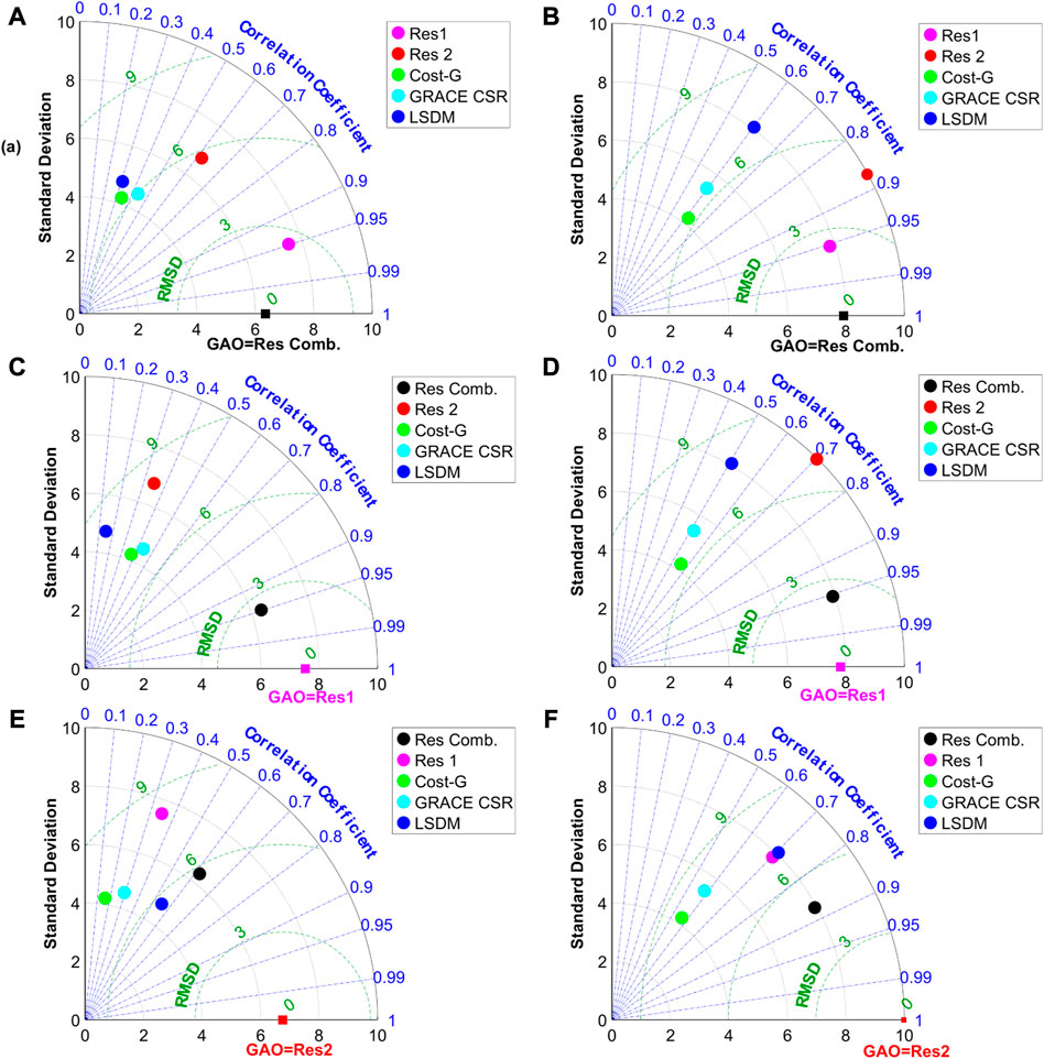
FIGURE 5. Taylor diagrams showing a comparison of χ₁ and χ₂ overall detrended components of three different geodetic residuals as a reference vlaues: (A) χ₁ of Res Comb. (B) χ₂ of Res Comb., (C) χ₁ of Res1, (D) χ₂ of Res1, (E) χ₁ of Res2, (F) χ₂ of Res2 with gravimetric-based excitation determined from a single GRACE/GRACE-FO solution (CSR), combined GRACE/GRACE-FO solution (COST-G), and HAM LSDM hydrological model.

χ₁ component of Res1 geodetic residuals, taken as observed value, is poorly explained by Res2, and GRACE/GRACE-FO based and HAM LSDM excitation functions alike (Figure 5C). None of the considered HAM excitations do not improve agreement with geodetic residuals Res1 in contrast to Res Comb (Figure 5A). The correlation of LSDM excitations with Res1 decreased to 0.15, and what is more, RMSD for both GRACE/GRACE-FO based excitations and LSDM HAM increase above 7.0 mas (see Figure 5C). For χ₂ component, an agreement between Res1 geodetic residuals and both GRACE/GRACE-FO based and HAM LSDM excitation, shown in Figure 5D, is slightly worse than for agreement with Res Comb. analyzed in 5 (b). Decreased correlations and increased RMSD between Res1 and hydrological signals indicate that agreement between the GRACE/GRACE-FO and HAM LSDM excitation is worse than for Res Comb. taken as a reference value.

Looking at Figure 5E, F, it is apparent that for Res2 geodetic residuals being reference value, the agreement between GRACE/GRACE-FO based solutions of CSR and COST-G is at the lowest level compared with previously referenced GAO excitations. It can be seen that both GRACE/GRACE-FO and HAM LSDM excitations still have too little spatial variability, where their standard deviation is as high as 4.1 to 4.9 mas in case of χ₁ component (Figure 5E), and 4.1 to 8.0 mas in case of χ₂ component (Figure 5F). Here, model LSDM has the best RMSD, equal 5.72 mas in χ₁, and 7.13 mas in χ₂, which is caused by the fact, that self-consistent AAM ECMWF, OAM MPIOM, and HAM LSDM excitation are derived from general circulation models outputs.

3.2.2 Seasonal and non-seasonal oscillations comparison

We now extend our research to analyzing seasonal and non-seasonal oscillations of geodetic residuals, Res1, Res2, and Res Comb., and GRACE/GRACE-FO-based gravimetric and hydrological excitations. Here, Chandler wobble and its anomalies are not under consideration. This is mainly because despite its large effect, the Chandler wobble excitation is just above the uncertainty level of the hydro-atmospheric Angular Momentum Functions (Bizouard, 2020). The equatorial angular momentum balance around Chandler frequencies deserves special treatment. Moreover, in the beggining of 2000s, the amplitude of the Chandler wobble began to decrease and, in 2017–2020, reached a historical low (Zotov et al., 2022b; a). The integration of the atmospheric and oceanic excitations cannot explain the absence of Chandler wobble in the recent decade (Zotov L. V. et al., 2022). In preliminary studies, Yamaguchi and Furuya (2023) suggest that the present AAM and OAM excitations are still not accurate enough to reproduce the recent Chandler wobble anomaly and that some other signals could be missing either in the AAM or OAM. These conclusions agree with our research, where the inaccuracy of different AAM and OAM models in the hydrological signal of polar motion is under consideration.

Here, the study are focusing on seasonal changes of hydrological signal in geodetically observed PM excitation - GAO and the analog signal present by GRACE/GRACE-FO data and HAM LSDM model. The analyzed seasonal oscillations in PM excitation is composed of a 1-year harmonic term, semi-annual and ter-annual terms.

Firstly, seasonal series obtained by fitting complex sinusoids with periods 365.25, 180.0, and 120.0 days to the overall series using least squares method was drawn on Figure 6. It can be seen that seasonal changes of different geodetic residuals, Res1, Res2, and Res Com., both GRACE/GRACE-FO based and LSDM excitations, are dominated by annual oscillation in χ₁ and χ₂ component. GRACE/GRACE-FO COST-G and CSR-based series are consistent with each other, but they visibly underestimate the amplitudes observed for different geodetic residuals and HAM LSDM. All geodetic residuals, Res1, Res2, and Res Comb., agree regarding their amplitudes, but some discrepancies are visible. The seasonal signal in PM excitation is mainly related to precipitation seasonality and changes in soil water content. This signal is generally more substantial in the χ₂ than in the χ₁ component cause of the higher dependence on mass changes on the continents of the Northern Hemisphere (Dobslaw et al., 2010). These findings are consistent with the conclusions shown based on Taylor Diagrams (Figure 7).

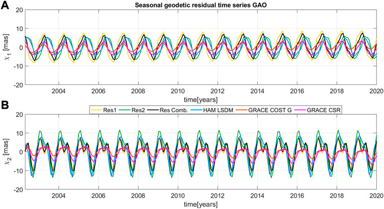
FIGURE 6. Comparison of seasonal oscillations of the equatorial components of the χ₁ (A) and χ₂ (B) geodetic residuals (Res1, Res2, Res Comb.) with gravimetric-based excitation determined from a single GRACE/GRACE-FO solution (CSR), combined GRACE/GRACE-FO solution (COST-G), and HAM LSDM hydrological model.

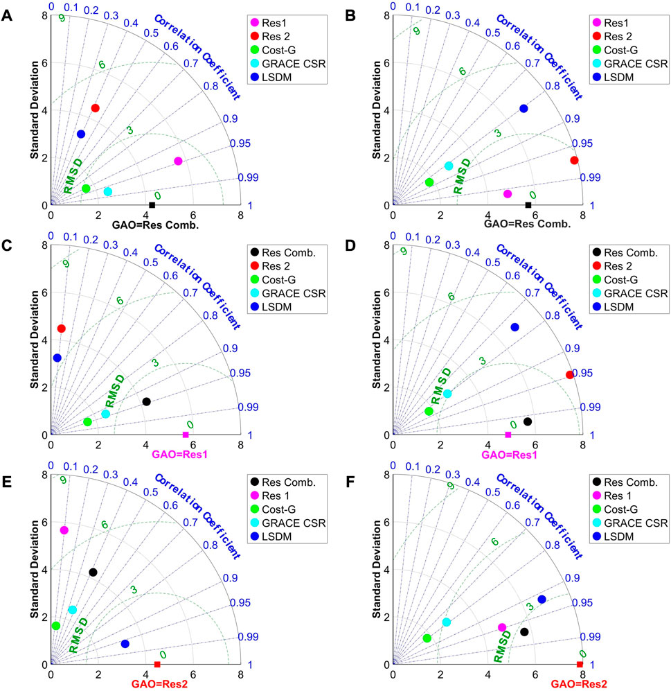
FIGURE 7. Taylor diagrams showing a comparison of χ₁ and χ₂ seasonal components of three different geodetic residuals as a reference vlaues: (A) χ₁ of Res Comb. (B) χ₂ of Res Comb., (C) χ₁ of Res1, (D) χ₂ of Res1, (E) χ₁ of Res2, (F) χ₂ of Res2, with gravimetric-based excitation determined from a single GRACE/GRACE-FO solution (CSR), combined GRACE/GRACE-FO solution (COST-G), and HAM LSDM hydrological model.

A Taylor diagram of the seasonal geodetic residuals Res1, and Res2, and GRACE/GRACE-FO based and HAM LSDM excitations is shown in Figure 7 (a) for χ₁, and (b) for χ₂ with referenced value referred to Res Comb. excitations. Only Res1 geodetic residuals demonstrate a similar ability to Res Comb, both in χ₁ (Figure 7A), and χ₂ (Figure 7B) component. In the χ₂ component, Res2 geodetic residuals correlate on 0.97, and their RMSD is equal to 2.75 mas, but it overestimates Res Comb. with STD of 7.87 mas. In the case of the χ₁ component, Res2 has the lowest correlation coefficient, among all considered time series, on the level of 0.41, and has the biggest RMSD equal 4.72 mas. This confirms a good consistency among seasonal geodetic residual time series developed with different AAM and OAM models and by the 3CH method, except Res2 χ₁ component. Seasonal HAM excitations computed from GRACE/GRACE-FO solutions, namely, CSR and COST-G, have the lowest RMSD, 2.11 mas for CSR, and 2.80 for COST-G in the χ₁ component. Their correlation coefficients are above 0.90, but standard deviations, around 2.0 mas, do not explain the right amplitude value of Res Comb., equal 4.26 mas (Figure 7A). In the case of χ₂ component, both GRACE/GRACE-FO based excitations underestimated Res Comb. however, their correlation coefficients are on the level of 0.82, and their standard deviations are as high as 3.84 mas and 4.27 mas for COST-G and CSR, respectively. The impact of fresh inland waters representing by HAM LSDM excites the seasonal polar motion at almost the same level (with STD equal 3.24 in χ₁, and 6.84 in χ₂) but does not permit to close of the budget of polar motion with a low correlation coefficient equal 0.38 and high RMSD (4.22 mas) in χ₁ component.

The agreement between Res1 geodetic residuals (reference value) and Res2, Res Comb. and GRACE/GRACE-FO based and HAM LSDM excitations of seasonal oscillations are shown in Figure 7C for χ₁ and (d) for χ₂ component. Here, large discrepancies between referenced Res1 and Res2 excitations are noted in the χ₁ component. Low correlation coefficient, 0.11, and high RMSD, 6.86 mas indicate that those geodetic residuals computed from various AAM, and OAM models, differ significantly in seasonal oscillations, although their pretty good agreement in standard deviation (Figure 7C). In the case of the χ₂ component, an agreement between Res1 and Res2 is very good. The correlation coefficient reaches the value of 0.94. RMSD is as high as 3.96 mas. However, in this case, the amplitude of referenced Res1 excitation is overestimated by the Res2 time series (Figure 7D).

Res1 geodetic residuals are slightly better explained in χ₂ component by both GRACE/GRACE-FO solutions in contrast to Res Comb. In contrast, it is worse explained by both GRACE/GRACE-FO based excitations in χ₁ component, where RMSD is higher than 3.00 mas for CSR and COST-G solutions. Very low compatibility in χ₁ seasonal component is noted for HAM LSDM excitations, where the correlation coefficient achieves 0.09 value, and RMSD exceeds 6.00 mas. In the case of χ₂, LSDM excitations agreed on the higher level in Res Comb. than in Res1.

Taking Res2 geodetic residuals as the observed value, it can be concluded from Figure 7E for χ₁ and (f) for χ₂ component that the highest agreement is with LSDM excitations with pattern correlation about 0.96, and 0.92, and RMSD about 1.61, and 3.16 mas, in χ₁, and χ₂ component, respectively. None of the GRACE/GRACE-FO based excitations explain seasonal oscillations of Res2 geodetic residuals better than Res Comb. and Res1 excitations.

To further study, seasonal variations were decomposed into annual prograde, annual retrograde, semi-annual prograde, and semi-annual retrograde parts, and their amplitudes and phases are presented in Table 3.

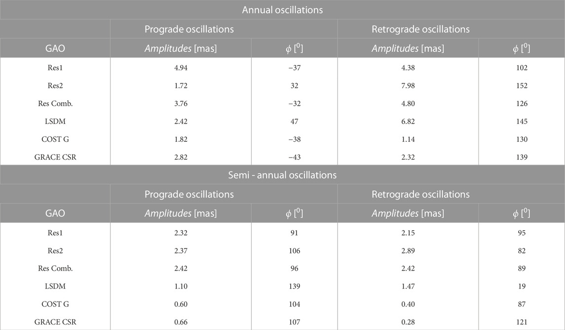
TABLE 3. Amplitudes and phases (ϕ) of prograde and retrograde both annual and semiannual oscillations of geodetic residuals (Res1, Res2, and Res Comb.), and of hydrological excitations computed from LSDM model and from GRACE data (COST-G and CSR solutions). Phase ϕ is defined here by the annual and semiannual term as $\sin \left(\right.2\pi (t-t_0)+\varphi$, where t₀ is a reference epoch for 1 January 2005.

From Table 3 can be concluded that the annual prograde and retrograde components of different geodetic residuals and GRACE/GRACE-FO based and HAM LSDM excitations are stronger than semiannual components. In general, gravimetric excitation series, COST G, and GRACE CSR underestimate annual amplitudes observed for all geodetic residuals except for the prograde annual amplitude of the Res2 solution. HAM LSDM excitation agrees, in terms of annual prograde and retrograde amplitudes and phases, with the Res2 solution based on the ECMWF+MPIOM atmosphere-ocean model consistent with the hydrological model.

The annual amplitude differences between combined geodetic residual solution, Res Comb., and other series are between 1.18 and 2.04 mas for the prograde term and between 3.18 and 3.66 mas for the retrograde term. In particular, GRACE CSR and COST-G-based series are characterized by the smallest amplitudes of prograde annual oscillations in contrast to combined geodetic residuals. Therefore, the use of this solution for the analysis of annual changes in hydrological part of PM excitation could be more favorable. On the other hand, Res2 prograde annual amplitude is equal to 1.72 and is as high as for GRACE/GRACE-FO and HAM LSDM excitations. Regarding the phases of annual oscillation, all geodetic residuals and GRACE/GRACE-FO based and HAM LSDM series present relatively compatible results with phase differences regarding Res Comb. within 11⁰-79⁰ for the prograde term and 24⁰-26⁰ for the retrograde term.

Similarly, semiannual prograde and semiannual retrograde oscillations show that amplitudes and phases of different geodetic residuals are in very good agreement. However, GRACE/GRACE-FO-based and HAM LSDM excitations amplitudes are very weak, and their phases are more varied than geodetic residuals. Because the amplitudes of ter-annual oscillations show very low values in comparison to annual and semi-annual ones, they were not presented in this paper.

In order to show the time changes of the considered Res1, Res2, Res Comb., HAM LSDM, and GRACE/GRACE-FO based excitation functions of polar motion, their time variable spectra were computed using the Fourier Transform Band Pass Filter (Kosek, 1995) in the broadband with 60–500 days cutoff and displayed on Figure 8. As shown in Figure 8, geodetic residual excitations of polar motion, Res1, Res2, Res Comb., hydrological (HAM LSDM), and gravimetric (Cost-G, CSR) excitations are irregular. Variable annual oscillations of the prograde and retrograde components are visible for all considered excitations, but gravimetric excitations (Cost-G solution) are the weakest. Semiannual and 120 - day signal oscillations are stronger for the geodetic residuals Res1, Res2, and Res Comb. than for hydrological and gravimetric excitations. Differences between time variable spectra computed for different geodetic residuals Res1, Res2, and Res Comb., are noticeable and may be affected by uncertainties introduced to geodetic residuals GAO by atmospheric and oceanic models (Chen et al.,2017). These differences may affect agreement in the so-called geodetic budget: total explanation of observed geodetic excitation of polar motion by hydro-atmosphere processes. The so-called geodetic budget is disturbed by the uncertainties of the AAM, OAM, and HAM models, the partial knowledge of the ocean-atmosphere coupling and hydrological processes, and discrepancies between models for wind terms and the current ocean terms as well. There is hope that by the progress made in recent decades, progress in global circulation models may improve their quality and consistency between different research centers.

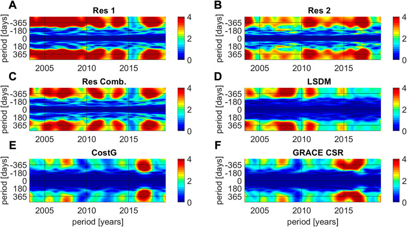
FIGURE 8. The time variable spectrum of the 60–500 days band of the geodetic residual excitations Res1 (A), Res2 (B), Res Comb. (C), HAM LSDM hydrological model (D), gravimetric-based excitation determined from a combined GRACE/GRACE-FO solution (COST-G) (E), and single GRACE/GRACE-FO solution (CSR) (F) (in mas).

The non-seasonal oscillations reveal all signals in PM after removing long-term changes and seasonal variations from the overall detrended time series, shown in Figure 9. The overall variability of non-seasonal residual series remains prominent, but significant differences occur. It can be seen that geodetic residuals have amplitudes as high as GRACE/GRACE-FO-based and HAM LSDM excitations. However, hydrological models and gravimetric data reveal imperfections in explaining the geodetic budget. Detailed analysis of non-seasonal agreement of different geodetic residuals and GRACE/GRACE-FO-based and HAM LSDM excitations is conducted through validation of time series with the use of the parameters shown in Figure 10.

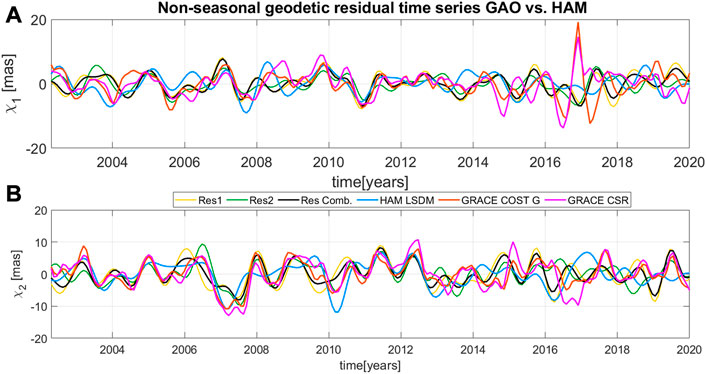
FIGURE 9. Comparison of non-seasonal oscillations of the equatorial components of the χ₁ (A) and χ₂ (B) geodetic residuals (Res1, Res2, Res Comb.) and for different hydrological-based excitations of polar motion (LSDM, COST-G, and CSR solutions).

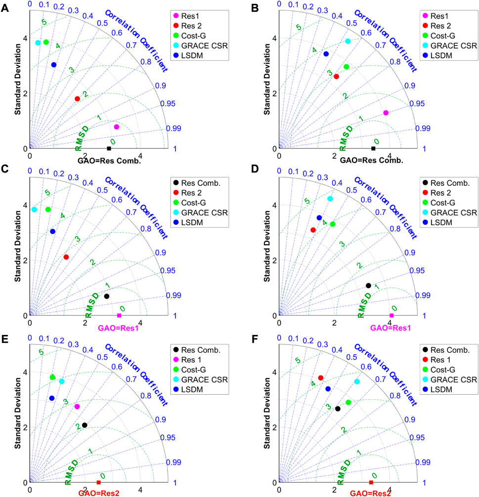
FIGURE 10. Taylor diagrams showing a comparison of χ₁ and χ₂ non-seasonal components of three different geodetic residuals as a reference vlaues: (A) χ₁ of Res Comb. (B) χ₂ of Res Comb., (C) χ₁ of Res1, (D) χ₂ of Res1, (E) χ₁ of Res2, (F) χ₂ of Res2, with gravimetric-based excitation determined from a single GRACE/GRACE-FO solution (CSR), combined GRACE/GRACE-FO solution (COST-G), and HAM LSDM hydrological model.

The relative merits of various GRACE/GRACE-FO based and LSDM excitations concerning Res Comb. geodetic residuals can be inferred from Figure 10 (a) for χ₁ and (b) for χ₂ component. It can be seen that other geodetic residuals, Res1, and Res2, generally agree better with Res Comb. than GRACE and HAM solutions, each with about similar standard deviations of 2.60 − 3.40 mas in χ₁, and 3.60 − 4.30 mas in χ₂ of non-seasonal oscillations. The amplitudes of various geodetic residuals are underestimated by each GRACE/GRACE-FO and LSDM excitations, both in χ₁ and χ₂ components. Generally, the χ₁ component is worse explained by GRACE/GRACE-FO based and LSDM excitations than the χ₂ component. Regardless of choice of referenced geodetic residuals, Res1, Res2, or Res Comb., the agreement between χ₁ geodetic residuals and other hydrological signal is poorer performed (Figures 10A, C, E ). In Figures 10B, D, F, it can be seen that GRACE/GRACE-FO based and LSDM excitations generally agree better with Res2 geodetic residuals, than with Res1, and Res Comb., each with about similar RMSD equal from 3.00 to 4.20 mas and correlation coefficients as high as 0.44–0.66.

The combined geodetic residual series processed with the 3CH method generally does not improve consistency between observed polar motion excitations and geophysical ones at non-seasonal time scales. However, Res Comb. ‘s agreement with GRACE and HAM LSDM hydrological signal is much better than that of Res1 with the hydrological signal. Still, other disruptive factors of mass changes in Earth’s system not modeled by hydrological models and not revealed in GRACE/GRACE-FO data do not permit to close of this budget.

4 Discussion and conclusion

In this study, different combinations of geodetic residuals, GAM-(AAM+OAM), were analyzed to estimate the total effect of atmospheric and oceanic excitations on PM compared to GRACE/GRACE-FO based and HAM LSDM excitations, considering complex-valued components (χ₁ + i χ₂). Res Comb. solution, being weighted arithmetic mean of six primary geodetic residuals computed from various mass and motion terms of AAM and OAM available models, was estimated by the 3CH method to find the best fit to HAM excitations. This resolution (Res Comb.) was characterized by minimized internal noise of different geodetic residual excitations (Res1 to Res6). Each geodetic residual model’s agreement was compared to each other at long-term variations and overall detrended, seasonal, and non-seasonal oscillations. It was found that all geodetic residuals computed from different combinations of mass and motion terms of AAM and OAM models play an essential role at broadband frequencies of polar motion, and differences between them can not be negligible. In addition, geodetic residuals based on various OAM models, the ECCO and MPIOM, differ significantly and show low correlations between themselves, which were also found in previous studies (Bizouard, 2020; Harker et al., 2021). Moreover, geodetic residuals, Res1 and Res4, differ only by the mass terms for both AAM models, NCEP/NCAR and ECMWF, showing high correlations between each other. However, some crucial differences between geodetic residuals based on various motion terms were found, which were also found in previous studies (Aoyama and Naito, 2000; Masaki, 2008).

Considering the differences between the geodetic residual excitations, this study aimed to build a criterion that would allow a less arbitrary choice of one geodetic residual GAO time series and compare it with HAM excitations. A quality criterion independent of HAM excitations was built, and the noise level of the various GAO series and one combination Res Comb. with a generalized 3CH method was estimated.

The agreement between the combined series, Res Comb., Res1, Res2, and GRACE/GRACE-FO based and HAM LSDM excitations were studied to determine the influence of a minimal noise level on agreement with different HAM. We noted that the combined geodetic residual time series presented a good overall agreement with GRACE COST-G, CSR, and HAM LSDM time series, much better than the comparison with Res1 and Res2 single solutions in a broad spectrum band (Figure 5). Here, Res2 geodetic residuals agree with GRACE/GRACE-FO and HAM LSDM solution the worst.

At seasonal time scales, Res1, Res2, and Res Comb. geodetic residuals show significant discrepancies, especially in the χ₁ component. Seasonal variations of GRACE COST-G and CSR solutions agree the best with Res Comb. geodetic residuals, both in χ₁ and χ₂ components. Seasonal Res2 time series agree best with HAM LSDM hydrological model since AAM ECMWF, OAM MPIOM, and HAM LSDM create a consistent set of geophysical excitations by stabilizing the sum of total masses in geophysical fluid layers.

The decomposition of seasonal variations into prograde and retrograde parts shows that the annual signal is the strongest. The annual amplitude differences between combined geodetic residuals, Res Comb., and other solutions are a couple of mas. All geodetic residuals and GRACE/GRACE-FO and HAM LSDM excitations present relatively congruous results regarding their phase agreement.

Seasonal time variable spectra of Res1, Res2, Res Comb., hydrological (HAM LSDM), and gravimetric (COST-G and CSR) are irregular. The signals of seasonal time variable spectra computed for various geodetic residuals, Res1, Res2, and Res Comb., are stronger than for hydrological signals computed from HAM LSDM and GRACE/GRACE-FO solutions. Differences between time variable spectra of different GAO are noticeable and may be affected by uncertainties introduced by AAm and OAM models.

The overall variability at the non-seasonal spectral band of different GAO and hydrological signals (HAM LSDM, GRACE/GRACE-FO) is prominent, but significant differences occur. Here, the combined geodetic residuals, Res Comb., do not improve consistency between observed geodetic polar motion and geophysical ones. Res2 agreement with GRACE/GRACE-FO and HAM LSDM solutions is the best.

The combined geodetic residual series processed with the 3CH method improves consistency between observed polar motion excitations and geophysical ones at overall and seasonal oscillations. Nevertheless, other disruptive factors of mass changes in Earth’s system not modeled by hydrological models and not revealed in GRACE/GRACE-FO data do not permit to close of the geodetic budget.

Data availability statement

The raw data supporting the conclusions of this article will be made available by the authors, without undue reservation.

Author contributions

MW contributed to conception and design of the study, organized the database, performed the statistical analysis, wrote the first draft of the manuscript, wrote sections of the manuscript, to manuscript revision, read, and approved the submitted version.

Funding

This paper was co-financed under the research grant of the Warsaw University of Technology supporting the scientific activity in the discipline of Civil Engineering and Transport.

Conflict of interest

The authors declare that the research was conducted in the absence of any commercial or financial relationships that could be construed as a potential conflict of interest.

Publisher’s note

All claims expressed in this article are solely those of the authors and do not necessarily represent those of their affiliated organizations, or those of the publisher, the editors and the reviewers. Any product that may be evaluated in this article, or claim that may be made by its manufacturer, is not guaranteed or endorsed by the publisher.

References

Adhikari, S., Caron, L., Steinberger, B., Reager, J. T., Kjeldsen, K. K., Marzeion, B., et al. (2018). What drives 20th century polar motion? Earth Planet. Sci. Lett. 502, 126–132. doi:10.1016/j.epsl.2018.08.059
Adhikari, S., and Ivins, E. R. (2016). Climate-driven polar motion: 2003-2015. Sci. Adv. 2, e1501693. doi:10.1126/sciadv.1501693
Aoyama, Y., and Naito, I. (2000). Wind contributions to the Earth’s angular momentum budgets in seasonal variation. J. Geophys. Res. Atmos. 105, 12417–12431. doi:10.1029/2000JD900101
Barnes, R. T. H., Hide, R., White, A. A., and Wilson, C. A. (1983). Atmospheric angular momentum fluctuations, length-of-day changes and polar motion. Proc. R. Soc. Lond. A. Math. Phys. Sci. 387, 31–73. doi:10.1098/rspa.1983.0050
Bizouard, C. (2020). Geophysical modelling of the polar motion. Berlin, Boston: De Gruyter. doi:10.1515/9783110298093
Bizouard, C., Lambert, S., Gattano, C., Becker, O., and Richard, J. Y. (2019). The IERS EOP 14C04 solution for Earth orientation parameters consistent with ITRF 2014. J. Geodesy 93, 621–633. doi:10.1007/s00190-018-1186-3
Brzeziński, A., Nastula, J., and Kołaczek, B. (2009). Seasonal excitation of polar motion estimated from recent geophysical models and observations. J. Geodyn. 48, 235–240. doi:10.1016/j.jog.2009.09.021
Brzeziński, A., and Nastula, J. (2002). Oceanic excitation of the chandler wobble. Adv. Space Res. 30, 195–200. doi:10.1016/S0273-1177(02)00284-3
Chao, B. F., and Au, A. Y. (1991). Atmospheric excitation of the Earth’s annual wobble: 1980–1988. J. Geophys. Res. Solid Earth 96, 6577–6582. doi:10.1029/91JB00041
Chen, J. L., Wilson, C. R., Chao, B. F., Shum, C. K., and Tapley, B. D. (2000). Hydrological and oceanic excitations to polar motion andlength-of-day variation. Geophys. J. Int. 141, 149–156. doi:10.1046/j.1365-246X.2000.00069.x
Chen, J. L., and Wilson, C. R. (2008). Low degree gravity changes from GRACE, Earth rotation, geophysical models, and satellite laser ranging. J. Geophys. Res. Solid Earth 113, B06402–B06409. doi:10.1029/2007JB005397
Chen, J. L., Wilson, C. R., Ries, J. C., and Tapley, B. D. (2013a). Rapid ice melting drives Earth’s pole to the east. Geophys. Res. Lett. 40, 2625–2630. doi:10.1002/grl.50552
Chen, J. L., Wilson, C. R., and Zhou, Y. H. (2012). Seasonal excitation of polar motion. J. Geodyn. 62, 8–15. doi:10.1016/j.jog.2011.12.002
Chen, J., Ries, J. C., and Tapley, B. D. (2021). Assessment of degree-2 order-1 gravitational changes from GRACE and GRACE Follow-on, Earth rotation, satellite laser ranging, and models. J. Geodesy 95, 38. doi:10.1007/s00190-021-01492-x
Chen, W., Li, J., Ray, J., and Cheng, M. (2017). Improved geophysical excitations constrained by polar motion observations and GRACE/SLR time-dependent gravity. Geodesy Geodyn. 8, 377–388. doi:10.1016/j.geog.2017.04.006.Geodesy
Chen, W., Ray, J., Shen, W., and Huang, C. (2013b). Polar motion excitations for an earth model with frequency-dependent responses: 2. Numerical tests of the meteorological excitations. J. Geophys. Res. Solid Earth 118, 4995–5007. doi:10.1002/jgrb.50313
Chen, W., and Shen, W. (2010). New estimates of the inertia tensor and rotation of the triaxial nonrigid Earth. J. Geophys. Res. Solid Earth 115, B12419. doi:10.1029/2009JB007094
Cheng, M., Ries, J. C., and Tapley, B. D. (2011). Variations of the Earth’s figure axis from satellite laser ranging and GRACE. J. Geophys. Res. Solid Earth 116, B01409. doi:10.1029/2010JB000850
Chin, T. M., Gross, R. S., and Dickey, J. O. (2005). Multi-reference evaluation of uncertainty in Earth orientation parameter measurements. J. Geodesy 79, 24–32. doi:10.1007/s00190-005-0439-0
Dickman, S. R. (2003). Evaluation of “effective angular momentum function” formulations with respect to core-mantle coupling. J. Geophys. Res. Solid Earth 108, 1603. doi:10.1029/2001JB001603
Dill, R., and Dobslaw, H. (2019). Seasonal variations in global mean sea level and consequences on the excitation of length-of-day changes. Geophys. J. Int. 218, 801–816. doi:10.1093/gji/ggz201
Dill, R. (2008). Hydrological model LSDM for operational Earth rotation and gravity field variations. Sci. Tech. Rep. 35, 8095. doi:10.2312/GFZ.b103-08095
Dobslaw, H., Dill, R., Grötzsch, A., Brzeziński, A., and Thomas, M. (2010). Seasonal polar motion excitation from numerical models of atmosphere, ocean, and continental hydrosphere. J. Geophys. Res. Solid Earth 115, B10406. doi:10.1029/2009JB007127
Dobslaw, H., and Dill, R. (2018). Predicting Earth orientation changes from global forecasts of atmosphere-hydrosphere dynamics. Adv. Space Res. 61, 1047–1054. doi:10.1016/j.asr.2017.11.044
Eubanks, T. M. (1993). Variations in the orientation of the earth. Contributions Space Geodesy Geodyn. Earth Dyn. 24, 1–54. doi:10.1029/GD024p0001
Ferreira, V. G., Montecino, H., Yakubu, C. I., and Heck, B. (2016). Uncertainties of the Gravity Recovery and Climate Experiment time-variable gravity-field solutions based on three-cornered hat method. J. Appl. Remote Sens. 10, 015015. doi:10.1117/1.jrs.10.015015
Fukumori, I., Raghunath, R., Fu, L. L., and Chao, Y. (1999). Assimilation of TOPEX/Poseidon altimeter data into a global ocean circulation model: How good are the results? J. Geophys. Res. Oceans 104, 25647–25665. doi:10.1029/1999JC900193
Galindo, F. J., and Palacio, J. (2003). Post-processing ROA data clocks for optimal stability in the ensemble timescale. Metrologia 40, S237–S244. doi:10.1088/0026-1394/40/3/301
Göttl, F., Schmidt, M., Seitz, F., and Bloßfeld, M. (2015). Separation of atmospheric, oceanic and hydrological polar motion excitation mechanisms based on a combination of geometric and gravimetric space observations. J. Geodesy 89, 377–390. doi:10.1007/s00190-014-0782-0
Gray, J., and Allan, D. (1974). “A method for estimating the frequency stability of an individual oscillator,” in Annual Symposium on Frequency Control, Atlantic City, NJ, USA, 29-31 May 1974 (IEEE), 243–246. doi:10.1109/FREQ.1974.200027
Gross, R. (2007). Earth rotation variations – long period. Treatise Geophys. 11, 239–294. doi:10.1016/B978-044452748-6.00057-2
Gross, R. S., Fukumori, I., Menemenlis, D., and Gegout, P. (2004). Atmospheric and oceanic excitation of length-of-day variations during 1980–2000. J. Geophys. Res. Solid Earth 109, 2432. doi:10.1029/2003JB002432
Gross, R. S. (2000). The excitation of the Chandler wobble. Geophys. Res. Lett. 27, 2329–2332. doi:10.1029/2000GL011450
Gross, R. S. (2016). “Theory of earth rotation variations,” in VIII hotine-marussi symposium on mathematical Geodesy. Editors N. Sneeuw, P. Novák, M. Crespi, and F. Sansò (Cham: Springer International Publishing), 41–46.
Grubbs, F. E. (1948). On estimating precision of measuring instruments and product variability. J. Am. Stat. Assoc. 43, 243–264. doi:10.1080/01621459.1948.10483261
Güntner, A. (2008). Improvement of global hydrological models using GRACE data. Surv. Geophys. 29, 375–397. doi:10.1007/s10712-008-9038-y
Hagemann, S., and Gates, L. D. (2003). Improving a subgrid runoff parameterization scheme for climate models by the use of high resolution data derived from satellite observations. Clim. Dyn. 21, 349–359. doi:10.1007/s00382-003-0349-x
Hagemann, S., and Gates, L. D. (2001). Validation of the hydrological cycle of ECMWF and NCEP reanalyses using the MPI hydrological discharge model. J. Geophys. Res. Atmos. 106, 1503–1510. doi:10.1029/2000JD900568
Harker, A. A., Schindelegger, M., Ponte, R. M., and Salstein, D. A. (2021). Modeling ocean-Induced rapid earth rotation variations: An update. J. Geodesy 95, 110. doi:10.1007/s00190-021-01555-z
Ince, E. S., Barthelmes, F., Reißland, S., Elger, K., Förste, C., Flechtner, F., et al. (2019). Icgem – 15 years of successful collection and distribution of global gravitational models, associated services, and future plans. Earth Syst. Sci. Data 11, 647–674. doi:10.5194/essd-11-647-2019
Jäggi, A., Meyer, U., Lasser, M., Jenny, B., Lopez, T., Flechtner, F., et al. (2023). “International combination Service for time-variable gravity fields (COST-G),” in Beyond 100: The next century in Geodesy (Cham: Springer International Publishing), 57–65.
Jean, Y., Meyer, U., and Jäggi, A. (2018). Combination of GRACE monthly gravity field solutions from different processing strategies. J. Geodesy 92, 1313–1328. doi:10.1007/s00190-018-1123-5
Jin, S., Chambers, D. P., and Tapley, B. D. (2010). Hydrological and oceanic effects on polar motion from GRACE and models. J. Geophys. Res. Solid Earth 115, B02403. doi:10.1029/2009JB006635
Jin, S., Hassan, A., and Feng, G. (2012). Assessment of terrestrial water contributions to polar motion from GRACE and hydrological models. J. Geodyn. Rotation 62, 40–48. doi:10.1016/j.jog.2012.01.009
Jungclaus, J. H., Fischer, N., Haak, H., Lohmann, K., Marotzke, J., Matei, D., et al. (2013). Characteristics of the ocean simulations in the Max Planck Institute Ocean Model (MPIOM) the ocean component of the MPI-Earth system model. J. Adv. Model. Earth Syst. 5, 422–446. doi:10.1002/jame.20023
Kalnay, E., Kanamitsu, M., Kistler, R., Collins, W., Deaven, D., Gandin, L., et al. (1996). The NCEP/NCAR 40-year reanalysis project. Bull. Am. Meteorological Soc. 77, 437–472. doi:10.1175/1520-0477(1996)077⟨0437:TNYRP⟩2.0.CO;2
Koot, L., Viron, O. d., and Dehant, V. (2006). Atmospheric angular momentum time-series: Characterization of their internal noise and creation of a combined series. J. Geodesy 79, 663–674. doi:10.1007/s00190-005-0019-3
Kosek, W. (1995). Time variable band pass filter spectra of real and complex-valued polar motion series. Artif. Satell. 24, 27–43.
Masaki, Y. (2008). Wind field differences between three meteorological reanalysis data sets detected by evaluating atmospheric excitation of Earth rotation. J. Geophys. Res. Atmos. 113, D07110. doi:10.1029/2007JD008893
Meyrath, T., and van Dam, T. (2016). A comparison of interannual hydrological polar motion excitation from GRACE and geodetic observations. J. Geodyn. 99, 1–9. doi:10.1016/j.jog.2016.03.011
Nastula, J., Paśnicka, M., and Kołaczek, B. (2011). Comparison of the geophysical excitations of polar motion from the period: 1980.0–2009.0. Acta Geophys. 59, 561–577. doi:10.2478/s11600-011-0008-2
Nastula, J., Ponte, R. M., and Salstein, D. A. (2007). Comparison of polar motion excitation series derived from GRACE and from analyses of geophysical fluids. Geophys. Res. Lett. 34, L11306. doi:10.1029/2006GL028983
Neef, L. J., and Matthes, K. (2012). Comparison of Earth rotation excitation in data-constrained and unconstrained atmosphere models. J. Geophys. Res. Atmos. 117, 16555. doi:10.1029/2011JD016555
Ponte, R. M. (1997). Oceanic excitation of daily to seasonal signals in earth rotation: Results from a constant-density numerical model. Geophys. J. Int. 130, 469–474. doi:10.1111/j.1365-246X.1997.tb05662.x
Salstein, D. A., Kann, D. M., Miller, A. J., and Rosen, R. D. (1993). The sub-bureau for atmospheric angular momentum of the international earth rotation Service: A meteorological data center with geodetic applications. Bull. Am. Meteorological Soc. 74, 67–80. doi:10.1175/1520-0477(1993)074<0067:tsbfaa>2.0.co;2
Seoane, L., Biancale, R., and Gambis, D. (2012). Agreement between Earth’s rotation and mass displacement as detected by GRACE. J. Geodyn. 62, 49–55. doi:10.1016/j.jog.2012.02.008
Seoane, L., Nastula, J., Bizouard, C., and Gambis, D. (2011). Hydrological excitation of polar motion derived from GRACE gravity field solutions. Int. J. Geophys. 2011, 1–10. doi:10.1155/2011/174396
Śliwińska, J., and Nastula, J. (2019). Determining and evaluating the hydrological signal in polar motion excitation from gravity field models obtained from kinematic orbits of LEO satellites. Remote Sens. 11, 1784. doi:10.3390/rs11151784
Śliwińska, J., Wińska, M., and Nastula, J. (2022). Exploiting the combined GRACE/GRACE-FO solutions to determine gravimetric excitations of polar motion. Remote Sens. 14, 6292. doi:10.3390/rs14246292
Śliwińska, J., Wińska, M., and Nastula, J. (2019). Terrestrial water storage variations and their effect on polar motion. Acta Geophys. 67, 17–39. doi:10.1007/s11600-018-0227-x
Tavella, P., and Premoli, A. (1994). Estimating the instabilities ofNClocks by measuring differences of their readings. Metrologia 30, 479–486. doi:10.1088/0026-1394/30/5/003
Taylor, K. E. (2001). Summarizing multiple aspects of model performance in a single diagram. J. Geophys. Res. Atmos. 106, 7183–7192. doi:10.1029/2000JD900719
Torcaso, F., Ekstrom, C., Burt, E., and Matsakis, D. (2000). Estimating the stability of N clocks with correlations. IEEE Trans. Ultrasonics, Ferroelectr. Freq. Control 47, 1183–1189. doi:10.1109/58.869064
Wahr, J. M. (1983). The effects of the atmosphere and oceans on the Earth’s wobble and on the seasonal variations in the length of day — Ii. Results. Geophys. J. Int. 74, 451–487. doi:10.1111/j.1365-246X.1983.tb01885.x
Wińska, M. (2022). A comparative study of interannual oscillation models for determining geophysical polar motion excitations. Remote Sens. 14, 147. doi:10.3390/rs14010147
Wińska, M., Nastula, J., and Kołaczek, B. (2016). Assessment of the global and regional land hydrosphere and its impact on the balance of the geophysical excitation function of polar motion. Acta Geophys. 64, 270–292. doi:10.1515/acgeo-2015-0041
Winska, M., Nastula, J., and Salstein, D. (2017). Hydrological excitation of polar motion by different variables from the GLDAS models. J. Geodesy 91, 1461–1473. doi:10.1007/s00190-017-1036-8
Yamaguchi, R., and Furuya, M. (2023). The first-time absence of the chandler wobble since 2015 and its implications for excitation processes. Avaliable At: https://www.altmetric.com/details/135271933.
Yan, H., Chen, W., and Yuan, L. (2015). Crustal vertical deformation response to different spatial scales of GRACE and GCMs surface loading. Geophys. J. Int. 204, 505–516. doi:10.1093/gji/ggv385
Yu, N., Ray, J., Li, J., Chen, G., Chao, N., and Chen, W. (2021). Intraseasonal variations in atmospheric and oceanic excitation of length-of-day. Earth Space Sci. 8, e2020EA001563. doi:10.1029/2020ea001563
Zhou, Y. H., Salstein, D. A., and Chen, J. L. (2006). Revised atmospheric excitation function series related to Earth’s variable rotation under consideration of surface topography. J. Geophys. Res. Atmos. 111, D12108. doi:10.1029/2005JD006608
Zotov, L., Bizouard, C., Shum, C., Zhang, C., Sidorenkov, N., and Yushkin, V. (2022a). Analysis of Earth’s polar motion and length of day trends in comparison with estimates using second degree Stokes coefficients from satellite gravimetry. Adv. Space Res. 69, 308–318. doi:10.1016/j.asr.2021.09.010
Keywords: geodetic excitations of polar motion, hydrological angular momentum, geodetic residuals, hydrological signal in polar motion, error analysis
Citation: Wińska M (2023) Geodetic residual time series: A combined series by minimization of their internal noise level. Front. Earth Sci. 11:1138410. doi: 10.3389/feart.2023.1138410
Received: 05 January 2023; Accepted: 13 February 2023;
Published: 27 February 2023.
Edited by:
Takashi Nakagawa, Kobe University, JapanReviewed by:
Jun'Ichi Okuno, Research Organization of Information and Systems, JapanPakize Küreç Nehbit, Kocaeli University, Türkiye
Copyright © 2023 Wińska. This is an open-access article distributed under the terms of the Creative Commons Attribution License (CC BY). The use, distribution or reproduction in other forums is permitted, provided the original author(s) and the copyright owner(s) are credited and that the original publication in this journal is cited, in accordance with accepted academic practice. No use, distribution or reproduction is permitted which does not comply with these terms.
*Correspondence: Małgorzata Wińska, malgorzata.winska@pw.edu.pl