Improvements to the Shaw-Type Absolute Palaeointensity Method

Introduction

The acquisition of absolute palaeointensity data is problematic. The minerals that carry magnetic remanence are prone to various types of alteration in nature and in the laboratory. The matrix can also alter to form new magnetic minerals. This alteration affects the original magnetic signal and can lead to inaccurate estimates of past field strength. The pre-requisite that reliable palaeomagnetic directions and ages are obtained from suitable rocks is followed by time-consuming experiments, which often yield low success rates. To aid the process, there are several different methods with which a palaeointensity can be determined. Of these, variants of the thermal Thellier method (Thellier and Thellier, 1959; Coe, 1967; Tauxe and Staudigel, 2004) remains the most robust for assemblages of non-interacting uniaxial SD grains, due to its explicit theoretical basis grounded in the work of Néel (1949). However, it does have disadvantages that may be overcome by using alternative techniques such as the Shaw method (Shaw 1974; Tsunakawa and Shaw 1994, Yamamoto et al., 2003).

The Thellier method can only be used to calculate a palaeointensity at temperatures below those at which alteration occurs. The primary magnetic remanence of ancient rocks is often carried by grains associated with high unblocking temperatures and any thermo-chemical alteration that may influence the primary remanence during heating in the laboratory is not usually corrected for. The method can also suffer from multidomain (MD) effects associated with a failure of Thellier’s laws of thermoremanence, causing non-linear Arai plots, which can lead to erroneous palaeointensity estimates (Levi and Merrill, 1976; Shcherbakov et al., 2001; Paterson, 2011). This can lead to significant problems because of an oft-present multi-slope phenomenon that is not easily-overcome, causing under/over-estimations of the field strength (Thomas and Piper 1992; Xu and Dunlop 2004; Smirnov et al., 2017).

Compared with other palaeointensity methods, the imparted laboratory remanence in a Shaw experiment is somewhat more analogous to that acquired in nature, in that it is acquired during a single cooling from above the Curie temperature rather than during multiple stepwise heating-cooling cycles with lower peak temperatures. In principle, this makes it less prone to the multidomain effects associated with blocking and unblocking of partial thermoremanent magnetisations, and is said to be domain-state independent (Biggin and Paterson, 2014). Repeated measurements (before and after heating) of anhysteretic remanent magnetisation (ARM) are used to correct any physiochemical alteration of the magnetic minerals; this allows palaeointensities to be calculated from a thermal remanent magnetisation (TRM) at higher temperatures that would otherwise be beyond the range of a Thellier experiment. However, it should be noted that heating above the Curie temperature (Tc) can induce alteration affecting the whole specimen. Additional uncertainties are associated with the Shaw method and its subsequent variations; in particular, the use of ARM as an analogous substitute for TRM, given the well-established grain size dependency of the ratio of ARM and TRM (Tanaka and Komuro, 2009).

The palaeointensity average for the past 0–5 Ma is also noticeably lower when using the Shaw method compared with the Thellier method according to the PINT database (v.2015.05; http://earth.liv.ac.uk/pint/; Biggin et al., 2015). This discrepancy requires that both methods be scrutinised for any systematic biases that they may introduce.

Here we aim to provide a practical evaluation of several aspects of the Shaw-DHT method using a large dataset of well-characterised samples. A base set of selection criteria are applied to all data, after which, two linearity parameters with varying selection criteria are applied to the palaeointensity slope and compared. These include the curvature parameter (|k′|; Paterson 2011; Paterson et al., 2014b) and the R² correlation coefficient (R²_corr; Paterson et al., 2016). R²_corr is the square of the Pearson correlation (R_corr) used in other Shaw palaeointensity studies (Yamamoto et al., 2003). The aim is to determine the most effective set of selection criteria and provide a quantitative measure of their accuracy and precision. We also examine any potential effects of varying the high-temperature hold durations used in the experimental heatings.

The Shaw Method

The Shaw method produces a palaeointensity estimate by comparing the alternating frequency (AF) demagnetisation spectra of a natural remanent magnetisation (NRM) with that of a TRM that is acquired in a single step. Alteration is measured by comparing the demagnetisation spectra of an ARM imparted prior to, and following the laboratory heating; the difference is calculated for each coercivity step and applied as a correction to the TRM (Figure 1).

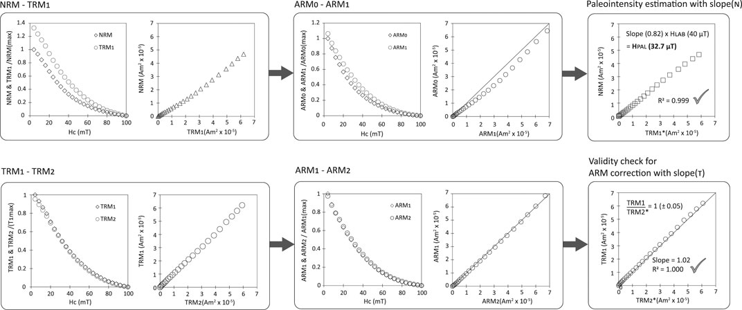
FIGURE 1. Schematic view of the data analyses process for the Shaw-type experiment using a specimen from Mount Etna. Top row is the palaeointensity experiment, where any alteration to the TRM₁ demagnetisation spectra is corrected by multiplying by the ARM slope (ARM₀/ARM₁) to produce TRM₁*. Bottom row is a repeat experiment to test the validity of the ARM corrections. This ARM validity check uses additional remanence acquisitions (TRM₂ and ARM₂) and should produce a unit slope. Note that the values shown in these figures are after vectoral subtraction of the remanences at the maximum AF step.

Originally proposed by Shaw (1974), the current method is the product of modifications that allow a palaeointensity to be calculated in the presence of alteration (Kono 1978; Rolph and Shaw 1985). The double heating technique (DHT) was further added (Tsunakawa and Shaw, 1994) with the purpose of testing the reliability of the ARM corrections. This involves a controlled repeat of the initial experiment, replacing the NRM with a laboratory TRM. If subsequent ARM corrections lead to the recovery the TRM, it suggests that the initial corrections are reliable.

The Shaw-DHT method (referred to as the Tsunakawa-Shaw method) now includes low-temperature demagnetisation (LTD; Yamamoto et al., 2003), which is said to preferentially remove remanence magnetisation held by MD grains (c.f. Ahn et al., 2016). The validity of the Shaw LTD-DHT method has been recognised in historical lavas (Yamamoto et al., 2003; Mochizuki et al., 2004; Oishi et al., 2005; Yamamoto and Hoshi, 2008) and in archaeological samples (Yamamoto et al., 2015).

The inclusion of LTD treatment is optional with respect to the theory behind the DHT. Recent studies of rocks that were moderately to highly MD (15–28%), obtained very similar palaeointensity estimates from LTD and non-LTD sister specimens (Yamamoto et al., 2007; Lloyd et al., 2021) and other studies successfully use the method without LTD. (Thallner et al., 2021). However, the incorporation of LTD can be important, not only for removing MD-like remanence, but also for the additional information it provides. The remanence loss due to LTD can be measured in the NRM, ARM and TRM steps; this can be used to quantify the size of the MD component, differences in the various remanent magnetisation losses and provide general information on how the LTD influences the coercivity spectra.

Here we outline the full experimental LTD-DHT method; note that the method requires an LTD treatment prior to demagnetising the NRM and TRMs (steps 1,3 and 5). These are then compared with the LTD treated ARMs (steps 2b, 4b and 6b; italics). The procedural steps are as follows:

1) (NRM) Stepwise AF demagnetisation of the NRM, usually up to 100–180 mT.

2a) (ARM₀) An ARM is imparted over the full coercivity range that was used in the NRM demagnetisation, and then progressively AF demagnetised using the same steps as for the NRM. The ARM direct current (DC) bias field is usually 2–3 times higher than the TRM DC bias field to compensate for a weaker ARM acquisition. The ARM AF demagnetising field must always equal the maximum AF demagnetisation step of the NRM.

2b) (ARM₀₀) LTD-ARM; the same as step 2a but with LTD treatment prior to AF demagnetisation.

3) (TRM₁) A TRM is imparted by heating in a magnetically shielded oven to above Tc (typically to 600^oC for magnetite), with heating and cooling in a constant DC bias field. This is then stepwise AF demagnetised to the same maximum level as the preceding steps. The DC bias field should be close to the expected palaeointensity or a sensible moderate value, i.e., 20 µT.

4a) (ARM₁) A second ARM is imparted over the full coercivity range, as before, and stepwise AF demagnetised to the same maximum level.

4b) (ARM₁₀) LTD-ARM; the same as step 4a but with LTD treatment prior to AF demagnetisation.

5) (TRM₂) A second TRM is imparted and demagnetised in an identical manner to step (3), usually with a longer hold duration.

6a) (ARM₂) A third ARM is imparted and demagnetised in an identical manner to steps (2a and 4a).

6b) (ARM₂₀) LTD-ARM; the same as step 6a but with LTD treatment prior to demagnetisation.

The key parameters obtained from a Shaw experiment are defined as follows:

• TRM₁*(i) = TRM₁(i) × [ARM₀(i)/ARM₁(i)]; TRM₁ is corrected at each AF demagnetisation step for the ARM₀/ARM₁ ratio at the same AF step.

• Slope_N (NRM/TRM₁^*) is the palaeointensity slope calculated using the corrected TRM₁.

• TRM₂*(i) = TRM₂(i) × [ARM₁(i)/ARM₂(i)]; TRM₂ is corrected at each AF demagnetisation step for the ARM₁

• ARM₂ ratio at the same AF step Slope_T (TRM₁/TRM₂^*) is the correction validation made using the slope between

• TRM₁ and the corrected TRM₂ and should be within 5% of unity.

The AF demagnetisation spectra used for all slopes corresponds to the coercivity range determined as the ChRM, except slope_T, which should use the full coercivity range or close to it, but no less than the ChRM.

Heating of samples are often conducted in a vacuum in order to repress high-temperature oxidation during laboratory heatings (Mochizuki et al., 2004). The Shaw LTD-DHT studies after Mochizuki et al. (2004) usually used vacuum heating.

The hold durations used for heating steps are chosen somewhat arbitrarily and have varied across different studies. It is common practice to prolong the second hold duration to allow a similar amount of alteration to occur in a specimen that has presumably undergone some thermal stabilisation. Some examples of first (second) heat hold durations are: 30 (60) minutes (Tsunakawa and Shaw, 1994), 10 (20) minutes (Yamamoto et al., 2003), 24 (48) minutes (Yamamoto and Hoshi, 2008), 20–35 (30–45) minutes (Mochizuki et al., 2011), 15 (30) minutes (Yamamoto and Yamaoka, 2018), and 30 (40) minutes (Okayama et al., 2019).

Specimens must be held above the Curie temperature of their remanence bearing minerals for enough time to homogeneously heat the specimen; however, heating durations have been shown to alter the ARM/TRM ratio and potentially affect the palaeointensity estimate (Tanaka and Komuro, 2009) and should therefore be subject to scrutiny.

ARM corrections are performed at each measurement point rather than applying a single correction obtained from the best fit slope of ARM₀/ARM₁; although the slope is a linear fit, the plot of ARM₀/ARM₁ need not be linear. This means that a unit slope does not necessarily mean that no alteration has taken place. In the results that will be discussed, we find that the curvature observed in slope_A (k′_A) tends to be inversely proportional to the difference in curvature between the corrected and uncorrected palaeointensity slope (∆k′), so that k′_A ≈ -∆k′ (Supplementary Figure S1). This is indicative of the non-linear behaviour of the ARM₀/ARM₁ data being transferred to the NRM/TRM* plot by the ARM correction.

Samples and Experimental Procedures

Monte Carlo Down-Sampling and Testing Linear Parameters

A large dataset of measurements undertaken on 426 individual specimens was compiled from multiple Shaw-DHT experiments, mostly carried out at the University of Liverpool over the last 3 years. Full multi-method palaeointensities are now published on many of these sample sets (Lloyd et al., 2021; Thallner et al., 2021). The experiments were performed using a wide variety of varying input parameters, including differences in the laboratory TRM bias field, ARM bias field, hold durations, sample positions, oven used and number of measurement steps. Most, but not all were heated in a vacuum, and many were subjected to LTD. treatment. Here, we do not test how LTD impacts on the palaeointensity estimates although this is something that could be done in the future.

The specimens (Table 1) vary widely in lithology and age, from present day lavas and igneous rocks reheated in the walls of a kiln, to Precambrian dolerite dykes and sills extending to more than 1Ga. These ancient samples are non-ideal recorders with various degrees of magnetominerological alteration. Included in the modern-day lavas are Shaw LTD-DHT data available in the MagIC database from a study on the andesitic lavas of Sakurajima (Yamamoto and Hoshi 2008). The deliberately large proportion of extremely non-ideal samples, which includes specimens that were originally determined to be unsuitable for palaeointensity based on rock magnetic results, is meant to ensure that the results represent a worst-case scenario.

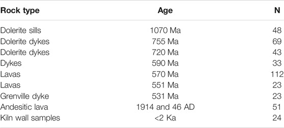
TABLE 1. Summary of all samples used in the dataset. Included are specimens from studies by Thallner et al., 2021 and Lloyd et al., 2021 (and other submitted work).

A simulated palaeointensity experiment was constructed (similar to Pan et al., 2002) by utilising the data from steps 3—6 of the standard Shaw-DHT method (see method description). A full TRM was imparted on all specimens, resetting their primary remanence and replacing it with a new thermal remanence (step 3 in the method description); importantly, this does not render them all thermally stable, since alteration is still observed in the majority of slopes A₂ (Supplementary Table S2). This laboratory induced TRM becomes the control that we aim to recover by comparing it with an additional, ARM corrected TRM (steps four to six in the method description). If a unit slope is produced when comparing the control TRM with the subsequent corrected TRM, the ARM correction is determined to be successful in exactly the same way as slope_T in a standard Shaw-DHT experiment.

The simulated palaeointensities produced here are the original slope_T values. The fundamental difference between this and a normal Shaw-DHT experiment is that here, there is no double heating; ARM corrections can be tested directly, whereas in the standard method, slope_T is an indirect test of the corrections performed in steps 1 and 2.

We begin by applying a base set of selection criteria to the entire dataset (Table 2), these include f_RESID (Paterson et al., 2016) which ensures that the palaeointensity slope is origin-trending, and the scatter parameter β (Coe et al., 1978), which is used to assess the slope uncertainty. After the base selection criteria are applied, the remaining data are randomly down-sampled ten thousand times with increasing number of specimens (N; starting at N = 3), as follows;

1. Three specimens are randomly sampled from the dataset, and this is repeated ten thousand times.

2. Every sampled specimen is analysed to determine a simulated palaeointensity (TRM₁/TRM₂*) using their full coercivity spectra.

3. For each set of three randomly sampled specimens, a mean palaeointensity and standard deviation is calculated. This produces ten thousand mean palaeointensities and standard deviations, each from an N of 3.

4. The ten thousand mean palaeointensities are sorted to calculate their 95% confidence limit and then averaged to produce an overall mean palaeointensity for an N of 3.

5. The ten thousand standard deviations are sorted to calculate their 95% confidence limit and then averaged to produce a mean standard deviation.

6. This iterative process is repeated, generating an overall mean palaeointensity and mean standard deviation with their respective 95% confidence limits for each increasing N. The accuracy and standard deviation of the mean is assessed as a function of N.

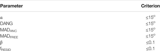
TABLE 2. Base set of selection that is applied to the entire dataset, and in addition to each of the parameters tested in this study. All parameters follow the Standard Palaeointensity Definitions (Paterson et al., 2014a).

After we establish a set of results using the base set of selection criteria, the entire process (steps 1–6) is repeated four more times, after various additional selection criteria are applied to the data. R²_corr is applied with two minima, R²_corr ≥ 0.990 and R²_corr ≥ 0.995; |k′| is also applied with two minima, |k′| ≤ 0.2 and |k′| ≤ 0.1. Each selection criterion is added individually to the base set of selection criteria and the results are randomly down-sampled ten thousand times each time, producing a total of five sets of down sampled results for comparison.

These parameters (R²_corr and |k′|) are used to assess Shaw plot linearity–the importance of strict linearity in the Shaw NRM-TRM₁* plot has previously been highlighted (Tanaka and Komuro, 2009) and is discussed further in Discussion.

Since all the specimens are thermally reset, the full coercivity range is used for all simulated palaeointensity slope fits; this removes any user bias that can result from the slope selection of a preferred coercivity range. Performance is measured by determining the number of specimens required to achieve an acceptable level (±10% of the correct mean) of accuracy and precision with 95% confidence.

The selection criteria are also compared using the published Sakurajima data (Yamamoto and Hoshi 2008). We are also able to determine how effective the DHT is at rejecting unreliable results in the same study because the expected field strength is known.

Testing the Double Heating Technique

The DHT is designed to provide additional confidence in the Shaw method; however, variations in the heating hold durations may influence the palaeointensity results that are obtained, particularly since TRM/ARM ratios have been demonstrated to evolve with excessive heating time (Tanaka and Komuro, 2009). Here, we examine the effect of varying experimental hold durations to determine if any heating time-dependency exists. To do this, we carried out a Shaw-DHT palaeointensity experiment on a set of 23 specimens, using hold durations that are shorter than usual whilst ensuring that equilibrium above Tc is reached. We then compared the slope_T values with sister specimens that underwent longer hold durations.

The samples from this experiment were from seven different sites and two different ages (five dolerite dykes aged 755 Ma and two sills aged 1070 Ma; Supplementary Table S1). The 23 half-inch length cylindrical cores were heated in a vacuum to 610°C and held for 15 min for the acquisition of both TRM₁ and TRM₂ (the second hold would normally be approximately twice as long). The TRMs were imparted using a 20 µT bias field. A third TRM was then imparted on three specimens from one site (MD6) to observe any differences in their AF demagnetisation spectra. The specimens were held at 610°C for 40 min using a 20 µT DC bias field.

Sister-specimens of the specimens used in this experiment yielded reversible high-temperature susceptibility curves (Supplementary Figure S2) and high-quality thermal Thellier results with a narrow distribution of remanence-bearing single-domain magnetite grains (Supplementary Figure S3). Their well-defined mineralogy and characteristics make them suitable to use in this comparison of hold duration effects.

Results

Whole Data Set Results

Results obtained after applying all of the selection criteria to the entire data set of 426 specimens (without down-sampling) are given in Table 3 and Supplementary Table S2. These simulated palaeointensity results are exactly equivalent to the slope_T values in the original experiments. Irrespective of the selection criteria used, an accurate mean palaeointensity is obtained (0.99–1.0). The standard deviations of results, however, differ considerably. Overall standard deviations range from 21% using only the base selection criteria to 9% for results with the additional criterion |k′| ≤ 0.1.

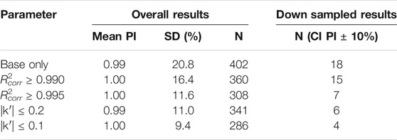
TABLE 3. Simulated palaeointensity results and standard deviations according to the selection criteria used. The base selection criteria (Table 2) are applied in all scenarios. Overall results: Mean PI, mean palaeointensity; SD (%), standard deviation; N, number of results to pass the selection criteria. Down sampled results: N (CI PI ± 10%), number of randomly sampled results required for the 95% confidence interval to be within 10% of the correct mean result (the lower the better).

Using |k′| with a threshold of ≤ 0.2 produces improved results to that of R²_corr ≥ 0.995 and notably improved over the results from R²_corr ≥ 0.990, which is widely used in current analyses (Table 2; Figures 2, 3). A further improvement is observed when decreasing the curvature minimum to ≤0.1, however, given that the difference is small, and its use may potentially discard specimens unnecessarily, we consider that a minimum acceptable curvature of ≤ 0.2 is optimal.

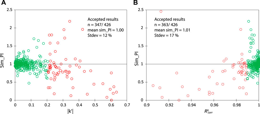
FIGURE 2. The full dataset of 426 simulated palaeointensity results are plotted against linearity parameters |k′| (A) and R²_corr(B). Here, no base selection criteria (Table 2) are applied before we plot the data, therefore, the values in these figures differ slightly to those in Table 3. Green circles, accepted results at the selected minima; red circles, rejected results at |k′| ≥0.2 and R²_corr ≤0.990. A few rejected results are not observed as they are outliers, falling outside the selected scale.

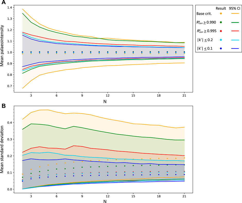
FIGURE 3. Plots of the down sampled results with increasing N, shown up to N = 21. (A) Mean palaeointensity (dots) are the (N) mean of ten thousand randomly sampled specimens, and associated 95% confidence interval (solid lines) results after applying each set of the tested selection criteria. (B) Mean standard deviation (dots) is the (N) mean of ten thousand randomly sampled specimens and associated 95% confidence interval (solid lines) results after applying each set of the tested selection criteria.

The results in Table 3 all have a base set of selection criteria (Table 2) applied to them, which remove 24 of the 426 results. In Figure 2, we compare the two linearity parameters with selected minima (R²_corr ≥ 0.990 and |k′| ≤ 0.2) on the full dataset of 426 specimens. No base selection criteria are applied in this comparison of the two parameters; therefore, the values differ slightly from those in Table 3. Use of the single criterion |k′| ≤ 0.2 appears to be more effective at rejecting non-ideal results, producing a mean result of 1.00 ± 0.12; this is compared to the criterion R²_corr ≥ 0.990 which rejects fewer specimens and produces a higher standard deviation (mean = 1.01 ± 0.17).

Down-Sampling Results

The Monte Carlo down-sampling also produced accurate mean palaeointensities, regardless of the number of specimens averaged (Figure 3A; Table 3 and Supplementary Table S3). All selection criteria yield an accurate mean intensity, but with varying scatter (standard deviation) and number of accepted results. Of the four sets with additional linearity checks, those that assess curvature yield the lowest result scatter (∼9–11%), while retaining 70–80% of the pre-screened results. When assessing plot curvature, we also observe consistently smaller numbers of specimens required to obtain a mean palaeointensity estimate that has a confidence interval within 10% of the mean. That is, using |k′| ≤ 0.2 or |k′| ≤ 0.1, in addition to the base selection criteria can yield a more precise palaeointensity estimate from fewer specimens (four to six specimens) than using the R²_corr (7–15 specimens). Furthermore, we observe that with our proposed selection we have a much smaller 95% confidence interval around the mean standard deviation (Figure 3B) which indicates that we can obtain a more constrained estimate of the data scatter than with other selection criteria.

True Palaeointensity Comparison

The selection criteria were also tested on the original Shaw LTD-DHT palaeointensity results from Sakurajima. The single linearity criterion (|k′| ≤0.2) was compared with the main two current Shaw-DHT selection criteria, (R²_corr ≥ 0.990 combined with slope_T = 1 ± 0.05; Yamamoto and Hoshi 2008). All specimen results pass the R²_corr and |k′| criteria; the only difference is due to the slope_T criterion, which causes six specimens to be rejected in the original published data (Figure 4A). Intensity error fractions for all but one of the rejected palaeointensity results are less than 8% and are closer to the expected geomagnetic field intensity than many of the successful results (Figure 4A). The results obtained using the single criterion |k′| are slightly improved over the current Shaw-DHT selection criteria (without the use of a second heating) in terms of the number of successful results, the mean palaeointensity result, and the standard deviation (Figure 4B).

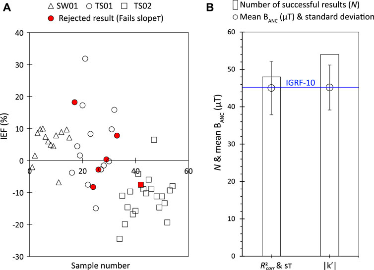
FIGURE 4. Palaeointensity results of the two volcanic lava flows from Sakurajima, (Yamamoto and Hoshi 2008). IGRF values are 45.7 and 46.0 µT. (A) All individual palaeointensity results using the current Shaw (LTD.)-DHT selection criteria. Results separated according to Yamamoto and Hoshi (2008). The only rejected results are due to a failure of the slope_T criterion (highlighted in red). IEF (%) is the intensity error fraction $=\left(\frac{m- \mu }{\mu } \text{X }100\right)$; m, estimated mean geomagnetic field intensity; µ, expected geomagnetic field intensity determined from IGRF-10 data. (B) A comparison of the results when applying the same Shaw-DHT selection criteria; R²_corr ≥ 0.990 and slope_T (sT) = 1 ± 0.05 (left) versus |k′| ≤0.2 (right). The blue horizontal line represents the mean expected palaeointensity according to IGRF-10.

Double Heating Technique Hold Time Results

As part of the original palaeointensity experiments that were carried out on the specimens in this study, one Shaw-DHT experiment was carried out on a subset that included specimens from seven different sites and three localities (Figure 5A). The experiment was designed to explore the effect of varying hold durations on the palaeointensity estimates and associated slope_T values. The effect of shorter hold durations on some slope_T values were not expected and are highlighted here. The slope_T values obtained were unusually high for several, but not all, specimens and they appear to cluster according to site (Figure 5A).

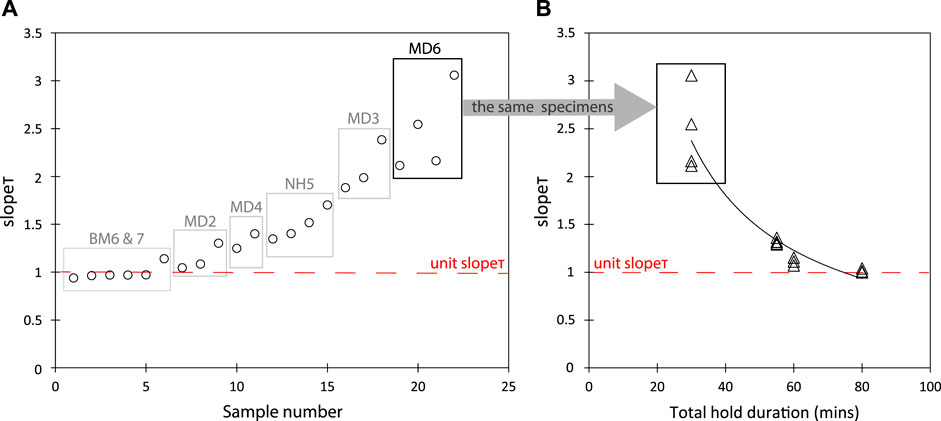
FIGURE 5. Comparison of slope_T results. (A) Results from a single Shaw-DHT experiment designed to test the effect of varying hold durations on palaeointensity estimates and slope_T values using hold durations of 15 min for TRM₁ and TRM₂. Values are plotted by site in ascending order. (B) Comparison of slope_T results from site MD6 as a function of total hold duration. The high slope_T values (boxed) are the same specimens from box in Figure 4A; these are compared with sister specimens from other Shaw-DHT experiments which had longer total hold durations.

We compared the high slope_T results from site MD6 with sister specimens that were subjected to longer hold durations, and noted that the values are affected by the hold duration used (Figure 5B). Sister specimens that underwent shorter hold durations (those in Figure 5A) produced high slope_T values. This is in contrast to sister specimens with a combined hold duration of 80 min, which produced a near unit slope_T (Figure 5B; Supplementary Figure S4).

It has recently been noted that Slope_T values may be dependent on hold duration (Lloyd et al., 2021); this is now further supported in more detail here. To analyse the cause of these latest observations, we subjected three of the specimens from site MD6 to a third TRM, heating to 610°C using a hold duration of 40 min and compared the AF demagnetisation spectra. In Figure 6 we show that a large decrease in the magnitude of TRM₂ is the cause of the high slope_T value in all three specimens, and this was brought about by the corresponding short hold duration (Figure 5B).

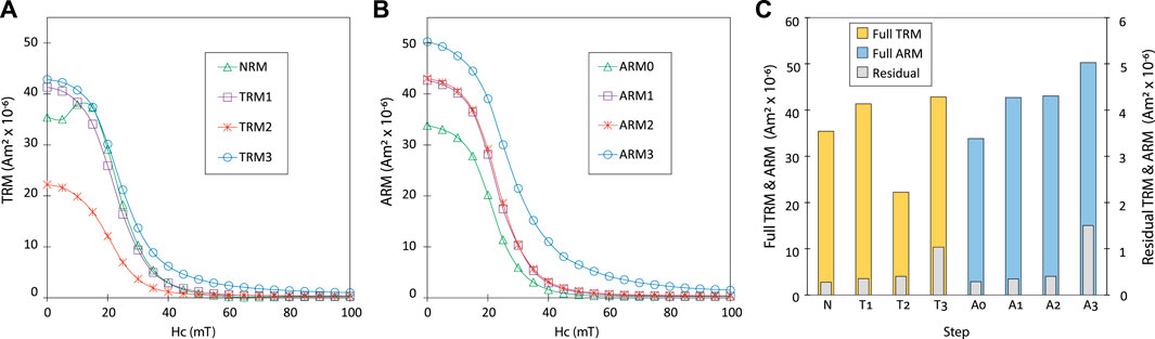
FIGURE 6. AF demagnetisation information for specimen 6.2A of site MD6. (A) Vector-subtracted TRM AF demagnetisation spectra. (B) Vector-subtracted ARM AF demagnetisation spectra. (C) Magnitudes of the remanence and residual magnetisations.

Alteration appears to have continued to affect TRM during the acquisition of TRM₃, but has caused a reversal of TRM magnitude which finishes close to the original TRM₁ position. The changes in demagnetisation spectra (Figure 6) infer that the heating would cause a change in slope_T (TRM₁—TRM₂* plot) depending on the time spent at high temperature. This result is in agreement with specimens from site MD6 that had longer hold durations and unit slope_T values (Figure 5). It is also worth noting that ARM appears to be unaffected by the apparent alteration to TRM.

Discussion

Summary of Results and Significance

Notably improved results are achieved by replacing the R²_corr with the curvature parameter |k′|. This is because it provides a more direct measure of linearity, the fundamental characteristic that should be tested for in the Shaw-type palaeointensity slope. A non-linear ARM-corrected Shaw palaeointensity slope suggests that changes in ARM are not behaving as an analogous substitute for TRM changes, most likely due to non-uniform high-temperature alteration affecting certain grain sizes (coercivity ranges) more than others. ARM/TRM ratios have previously been shown to differ with grain size and heating times (Tanaka and Komuro, 2009). The R²_corr parameter does not perform as well because it has a strong dependence on the number of points selected in the best-fit slope, which allows for increased curvature for a larger number of points. It can also be sensitive to random noise, which can decrease correlation despite a general linear trend in the data. In this sense, R²_corr measure both NRM-TRM reciprocity (i.e., linearity) as well as data scatter. We argue it is more appropriate to use two criteria more attuned to testing for reciprocity and scatter separately. For example combining curvature (|k′|) with the β parameter; The ratio of the standard error of the slope to the absolute value of the slope (Coe et al., 1978; Paterson et al., 2014a). These data pass the β minimum as part of the base selection criteria which suggests that the noise is acceptable.

The results based on using |k′| as a primary selection criterion are improved over existing data selection. The notable improvement in accuracy and precision when using |k′| ≤ 0.2 instead of R² ≥0.990 does not come at the expense of a lower success rate; these remain similar at 350 and 329 respectively from a potential 426; this is because the R²_corr criterion is rejecting more of the accurate palaeointensities than the |k′| criterion. The improved results are also obtained without a second heating (viewed as though the simulated experiment data were from an initial heating) and therefore, without using the DHT.

With the use of modern equipment such as a Rapid 2G, this new version of the method, with improved palaeointensity slope selection criteria (|k′|, f_RESID, β) and without the DHT, can be almost fully automated and able to produce as many as 100 palaeointensity and directional results per week using high resolution AF steps, while other more time-consuming methods may take up to ten times longer.

Observations on the Double Heating Technique

The validity of the DHT for natural rocks has been discussed by Tsunakawa and Shaw (1994) using historical or young lavas, where it was found to detect non-ideal behaviour or non-unity in the slope of TRM₁-TRM₂* plots. The results from such specimens were viewed as unreliable because they could potentially give an erroneous slope in the NRM-TRM₁* plots (Tsunakawa and Shaw, 1994; Yamamoto et al., 2003).

The initial findings presented in this study, however, suggest that it may be possible for the DHT to allow alteration to occur undetected in certain samples and that slope_T values could potentially be dependent on the hold duration used (c.f. Lloyd et al., 2021). This is highlighted in Figure 5B where sister specimens with varying hold durations produced very different slope_T values.

TRM and ARM can both be affected independently by alteration (Tsunakawa and Shaw, 1994; Tanaka and Komuro, 2009), which is demonstrated by the existence of non-unit slope_T values. The magnitude of their remanent magnetisation can also increase and decrease in the same experiment however (Figure 6). These results are preliminary, and require further study to understand the cause of, and extent to which the observed phenomena can occur; however, the reversibility of remanent magnetisation magnitudes after prolonged heating may not be uncommon. We often see results where slope_A1 and slope_A2 are opposite in magnitude, where the ARM slopes are less than and more than one, or vice versa (e.g., Yamamoto and Tsunakawa, 2005; Yamamoto et al., 2007); this implies that the ARM magnitudes are reversing. If slope_A1 (ARM₀/ARM₁) < 1, the heating has caused an overall increase in ARM over the coercivity steps used; if then, the slope_A2 (ARM₁/ARM₂) > 1, the ARM magnitude is altering in the opposite sense during the second heating. It is also possible that this occurs undetected in a single heating.

The cause of reversing magnitude in TRM and or ARM, which can occur in either remanence independently, is unclear. The loss of TRM observed in Figure 6 may be due to the oxidation of magnetite to hematite, however, this does not explain the subsequent increase in TRM₃. It is possible for new minerals to form that will acquire an increased TRM, but with coercivities too high to contribute to the ARM. This may account for the slight increase in residual magnetisation observed in TRM₃ (Supplementary Figure S5), but does not explain the reversing magnitude of the full TRM, which appears to require more than one mechanism.

A requirement of the Shaw-DHT method is that sufficient alteration occurs in the second heating in order to validate the initial ARM corrections. It is this second alteration correction that provides an indication of whether ARM and TRM are acting as analogues within the specimen. There are currently no criteria to prevent a specimen from becoming thermally stable during the first heating (alteration has saturated), which is inferred by a non-unit slope_A1 combined with a unit slope_A2 (e.g., Yamamoto and Tsunakawa 2005; Yamamoto et al., 2007). Where a specimen experiences little to no initial alteration, it should be expected to behave similarly in the subsequent heating, in which case, both slope_A1 and slope_A2 should be close to unity.

The technique also tends to remove accurate palaeointensity results, rather than outliers in the original Sakurajima palaeointensity study (Figure 4A); in this case it appears to say little about the accuracy of the palaeointensity estimate. It should be acknowledged, however, that any criterion designed for rejecting inaccurate estimates, can reject some of the accurate estimates.

An alternative and arguably more useful technique to test the validity of the alteration corrections would be to vary hold durations with sister specimens during their one and only heating. This enables a more direct assessment of alteration effects and ARM corrections at the palaeointensity level of the experiment, rather than the assessment coming from separate ARM corrections after further and excessive heating. Variations in palaeointensity values from sister specimens can be quantified and large standard deviations can be rejected.

Conclusions

We have identified a set of improved selection criteria for the Shaw-type palaeointensity method by down-sampling simulated palaeointensity results from a large dataset of 426 individual specimens. Use of the improved selection criteria demonstrate notably increased accuracy and precision of mean palaeointensity results. This comes with only a minor reduction in the number of successful results and, importantly, without the use of a second heating. We also highlight an additional measure as a safeguard to detect undesirable behaviour that requires varying the hold duration in sister specimens; however, the exact usage and interpretation of this approach requires further investigation.

We find that the DHT may allow alteration to occur undetected, and that slope_T appears to be dependent on the hold durations used in certain instances. In the analysis of historical lavas from Sakurajima, the effectiveness of the DHT was not demonstrated. We therefore suggest that a larger scale study of the DHT efficacy is required. The results suggest that it may not be necessary to include the DHT, however, more work is needed to better understand the broad spectrum of how alteration affects remanence magnetisations in the method. The removal of the DHT allows the method to be carried out much more expeditiously and almost fully automated if used in conjunction with modern equipment such as the Rapid 2G system.

Data Availability Statement

The original contributions presented in the study are included in the article/Supplementary Materials, further inquiries can be directed to the corresponding author.

Author Contributions

SL and DT carried out most of the experiments, SL derived many of the key concepts and wrote the manuscript. GP and AB advised, provided support and expertise at each step of the process. DT provided all the coding required to process the data and to run the down-sampling.

Funding

SL and AB acknowledge funding from the Leverhulme Trust (RLA-2016-080), GP is funded by a Natural Environment Research Council (NERC) Independent Research Fellowship (NE/P017266/1).

Conflict of Interest

The authors declare that the research was conducted in the absence of any commercial or financial relationships that could be construed as a potential conflict of interest.

Publisher’s Note

All claims expressed in this article are solely those of the authors and do not necessarily represent those of their affiliated organizations, or those of the publisher, the editors and the reviewers. Any product that may be evaluated in this article, or claim that may be made by its manufacturer, is not guaranteed or endorsed by the publisher.

Acknowledgments

The authors acknowledge Anna Holloway for measuring 24 of the samples used in this study, as part of her undergraduate dissertation. We also acknowledge the two anonymous reviewers for their valuable input into the manuscript.

Supplementary Material

The Supplementary Material for this article can be found online at: https://www.frontiersin.org/articles/10.3389/feart.2021.701863/full#supplementary-material

References

Ahn, H.-S., Kidane, T., Yamamoto, Y., and Otofuji, Y.-i. (2016). Low Geomagnetic Field Intensity in the Matuyama Chron: Palaeomagnetic Study of a Lava Sequence from Afar Depression, East Africa. Geophys. J. Int. 204, 127–146. doi:10.1093/gji/ggv303
Biggin, A. J., and Paterson, G. A. (2014). A New Set of Qualitative Reliability Criteria to Aid Inferences on Palaeomagnetic Dipole Moment Variations through Geological Time. Front. Earth Sci. 2, 1–9. doi:10.3389/feart.2014.00024
Biggin, A. J., Piispa, E. J., Pesonen, L. J., Holme, R., Paterson, G. A., Veikkolainen, T., et al. (2015). Palaeomagnetic Field Intensity Variations Suggest Mesoproterozoic Inner-Core Nucleation. Nature 526, 245–248. doi:10.1038/nature15523
Coe, R. S., Grommé, S., and Mankinen, E. A. (1978). Geomagnetic Paleointensities from Radiocarbon-Dated Lava Flows on Hawaii and the Question of the Pacific Nondipole Low. J. Geophys. Res. 83, 1740–1756. doi:10.1029/jb083ib04p01740
Coe, R. S. (1967). The Determination of Paleo-Intensities of the Earth's Magnetic Field with Emphasis on Mechanisms Which Could Cause Non-ideal Behavior in Thellier's Method. J. Geomagn. Geoelec. 19, 157–179. doi:10.5636/jgg.19.157
Kono, M. (1978). Reliability of Palaeointensity Methods Using Alternating Field Demagnetization and Anhysteretic Remanence. Geophys. J. Int. 54, 241–261. doi:10.1111/j.1365-246X.1978.tb04258.x
Levi, S., and Merrill, R. T. (1976). A Comparison of ARM and TRM in Magnetite. Earth Planet. Sci. Lett. 32, 171–184. doi:10.1016/0012-821X(76)90056-X
Lloyd, S. J., Biggin, A. J., Halls, H., and Hill, M. J. (2021). First Palaeointensity Data from the Cryogenian and Their Potential Implications for Inner Core Nucleation Age. J. Geophys. Res. 226, 66–77. doi:10.1093/gji/ggab090
Mochizuki, N., Oda, H., Ishizuka, O., Yamazaki, T., and Tsunakawa, H. (2011). Paleointensity Variation across the Matuyama-Brunhes Polarity Transition: Observations from Lavas at Punaruu Valley, Tahiti. J. Geophys. Res. 116, 1–17. doi:10.1029/2010JB008093
Mochizuki, N., Tsunakawa, H., Oishi, Y., Wakai, S., Wakabayashi, K.-i., and Yamamoto, Y. (2004). Palaeointensity Study of the Oshima 1986 Lava in Japan: Implications for the Reliability of the Thellier and LTD-DHT Shaw Methods. Phys. Earth Planet. Interiors 146, 395–416. doi:10.1016/j.pepi.2004.02.007
Néel, L. (1949). Théorie du Traînage Magnétique des Ferromagnétiques en Grains Fins Avec Application aux Terres 5 Cuites. Ann. Géophysique 5, 99–136
Oishi, Y., Tsunakawa, H., Mochizuki, N., Yamamoto, Y., Wakabayashi, K.-I., and Shibuya, H. (2005). Validity of the LTD-DHT Shaw and Thellier Palaeointensity Methods: A Case Study of the Kilauea 1970 Lava. Phys. Earth Planet. Interiors 149, 243–257. doi:10.1016/j.pepi.2004.10.009
Okayama, K., Mochizuki, N., Wada, Y., and Otofuji, Y.-i. (2019). Low Absolute Paleointensity during Late Miocene Noma Excursion of the Earth's Magnetic Field. Phys. Earth Planet. Interiors 287, 10–20. doi:10.1016/j.pepi.2018.12.006
Pan, Y., Shaw, S., Shaw, S., Zhu, R., and Hill, M. J. (2002). Experimental Reassessment of the Shaw Paleointensity Method Using Laboratory-Induced Thermal Remanent Magnetization. J. Geophys. Res. Solid Earth 107, EPM 1-1-EPM 1–10. doi:10.1029/2001jb000620
Paterson, G. A. (2011). A Simple Test for the Presence of Multidomain Behavior during Paleointensity Experiments. J. Geophys. Res. 116, 1–12. doi:10.1029/2011JB008369
Paterson, G. A., Heslop, D., and Pan, Y. (2016). The Pseudo-thellier Palaeointensity Method: New Calibration and Uncertainty Estimates. Geophys. J. Int. 207, 1596–1608. doi:10.1093/gji/ggw349
Paterson, G. A., Tauxe, L., Biggin, A. J., Shaar, R., and Jonestrask, L. C. (2014a). On Improving the Selection of Thellier-type Paleointensity Data. Geochem. Geophys. Geosyst. 15, 1180–1192. doi:10.1002/2013gc005135
Paterson, G. A., Tauxe, L., Biggin, A. J., Shaar, R., and Jonestrask, L. C. (2014b). Standard Paleointensity Definitions v1.1. 0–43. Available at: http://www.paleomag.net/SPD/spdweb.html.
Rolph, T. C., and Shaw, J. (1985). A New Method of Palaeofield Magnitude Correction for Thermally Altered Samples and its Application to Lower Carboniferous Lavas. Geophys. J. Int. 80, 773–781. doi:10.1111/j.1365-246x.1985.tb05124.x
Shaw, J. (1974). A New Method of Determining the Magnitude of the Palaeomagnetic Field: Application to Five Historic Lavas and Five Archaeological Samples. Geophys. J. Int. 39, 133–141. doi:10.1111/j.1365-246X.1974.tb05443.x
Shcherbakov, V. P., Shcherbakova, V. V., and Vinogradov, Y. K. (2001). On a Thermomagnetic Criterion for the Identification of the Domain Structure. Izv. - Phys. Solid Earth 70, 243–247. doi:10.1016/0031-9201(92)90190-7
Smirnov, A. V., Kulakov, E. V., Foucher, M. S., and Bristol, K. E. (2017). Intrinsic Paleointensity Bias and the Long-Term History of the Geodynamo. Sci. Adv. 3, e1602306–8. doi:10.1126/sciadv.1602306
Tanaka, H., and Komuro, N. (2009). The Shaw Paleointensity Method: Can the ARM Simulate the TRM Alteration? Phys. Earth Planet. Interiors 173, 269–278. doi:10.1016/j.pepi.2009.01.003
Tauxe, L., and Staudigel, H. (2004). Strength of the Geomagnetic Field in the Cretaceous normal Superchron: New Data from Submarine Basaltic Glass of the Troodos Ophiolite. Geochem. Geophys. Geosyst. 5, a–n. doi:10.1029/2003GC000635
Thallner, D., Biggin, A. J., and Halls, H. C. (2021). An Extended Period of Extremely Weak Geomagnetic Field Suggested by Palaeointensities from the Ediacaran Grenville Dykes (SE Canada). Earth Planet. Sci. Lett. 568, 117025. doi:10.1016/j.epsl.2021.117025
Thellier, E., and Thellier, O. (1959). Sur l’intensité du champ magnétique terrestre dans le passé historique et géologique. Ann. Géophysique 15, 285–376.
Thomas, D. N., and Piper, J. D. A. (1992). A Revised Magnetostratigraphy for the Mid-proterozoic Gardar Lava Succession, South Greenland. Tectonophysics 201, 1–16. doi:10.1016/0040-1951(92)90172-3
Tsunakawa, H., and Shaw, J. (1994). The Shaw Method of Palaeointensity Determinations and its Application to Recent Volcanic Rocks. Geophys. J. Int. 118, 781–787. doi:10.1111/j.1365-246X.1994.tb03999.x
Xu, S., and Dunlop, D. J. (2004). Thellier Paleointensity Theory and Experiments for Multidomain Grains. J. Geophys. Res. 109, 1–13. doi:10.1029/2004JB003024
Yamamoto, Y., and Hoshi, H. (2008). Paleomagnetic and Rock Magnetic Studies of the Sakurajima 1914 and 1946 Andesitic Lavas from Japan: A Comparison of the LTD-DHT Shaw and Thellier Paleointensity Methods. Phys. Earth Planet. Interiors 167, 118–143. doi:10.1016/j.pepi.2008.03.006
Yamamoto, Y., Torii, M., and Natsuhara, N. (2015). Archeointensity Study on Baked clay Samples Taken from the Reconstructed Ancient kiln: Implication for Validity of the Tsunakawa-Shaw Paleointensity Method. Earth Planet. Sp 67, 1–13. doi:10.1186/s40623-015-0229-8
Yamamoto, Y., and Tsunakawa, H. (2005). Geomagnetic Field Intensity during the Last 5 Myr: LTD-DHT Shaw Palaeointensities from Volcanic Rocks of the Society Islands, French Polynesia. Geophys. J. Int. 162, 79–114. doi:10.1111/j.1365-246X.2005.02651.x
Yamamoto, Y., Tsunakawa, H., Shaw, J., and Kono, M. (2007). Paleomagnetism of the Datong Monogenetic Volcanoes in China: Paleodirection and Paleointensity during the Middle to Early Brunhes Chron. Earth Planet. Sp 59, 727–746. doi:10.1186/BF03352736
Yamamoto, Y., Tsunakawa, H., and Shibuya, H. (2003). Palaeointensity Study of the Hawaiian 1960 Lava: Implications for Possible Causes of Erroneously High Intensities. Geophys. J. Int. 153, 263–276. doi:10.1046/j.1365-246X.2003.01909.x
Keywords: palaeointensity, palaeomagnetism, geomagnetism, thermal remanence, methodology
Citation: Lloyd SJ, Paterson GA, Thallner D and Biggin AJ (2021) Improvements to the Shaw-Type Absolute Palaeointensity Method. Front. Earth Sci. 9:701863. doi: 10.3389/feart.2021.701863
Received: 28 April 2021; Accepted: 16 July 2021;
Published: 29 July 2021.
Edited by:
Fabio Florindo, Istituto Nazionale di Geofisica e Vulcanologia (INGV), ItalyReviewed by:
Maxwell Christopher Brown, University of Minnesota, United StatesNobutatsu Mochizuki, Kumamoto University, Japan
Copyright © 2021 Lloyd, Paterson, Thallner and Biggin. This is an open-access article distributed under the terms of the Creative Commons Attribution License (CC BY). The use, distribution or reproduction in other forums is permitted, provided the original author(s) and the copyright owner(s) are credited and that the original publication in this journal is cited, in accordance with accepted academic practice. No use, distribution or reproduction is permitted which does not comply with these terms.
*Correspondence: Simon J. Lloyd, s.lloyd@liverpool.ac.uk