Distributed Melt on a Debris-Covered Glacier: Field Observations and Melt Modeling on the Lirung Glacier in the Himalaya

Introduction

Debris-covered glaciers are common in a number of glaciated mountain ranges, including high-mountain Asia [HMA, (Scherler et al., 2011)], the European Alps (Brock et al., 2010), the Caucasus (Lambrecht et al., 2011), the Andes of Chile (Janke et al., 2015) and Peru (Wigmore and Mark 2017), and the Russian (Barr et al., 2018), North American (Herreid and Pellicciotti 2018) and Scandinavian Arctic (Midgley et al., 2018). In HMA, they represent a considerable portion of the entire glacierized area (11%) and of the ice mass below the equilibrium line altitude (30%, Bolch et al., 2012; Kraaijenbrink et al., 2017), which is largely due steep hillslopes and high erosion rates.

Debris cover controls melt, with debris beyond a couple of centimeters in thickness inhibiting melt (Östrem, 1959; Nicholson and Benn 2006) and thinner cover increasing melt due to a decrease in albedo. A number of recent studies found debris-covered and clean ice glacier tongues to have comparable surface lowering rates on the glacier scale (Gardelle et al., 2012; Kääb et al., 2012; Nuimura et al., 2012; Basnett et al., 2013), while point scale observational studies have documented reduced melt below a critical thickness of few centimeters of debris (Loomis 1970; Khan 1989; Kayastha et al., 2000; Nicholson and Benn 2006; Lambrecht et al., 2011; Chand et al., 2015).

A number of studies have since investigated melt of debris-covered tongues in detail. Studies in the Alps and HMA have shown that energy balance models perform well to estimate melt at the point scale. However these models are very sensitive to thickness, thermal conductivity and surface roughness of the debris layer, all of which are difficult to measure (Nicholson and Benn 2006; Reid and Brock 2010; Rounce et al., 2015). A number of studies have also observed and modeled melt of supraglacial ice cliffs (Sakai et al., 2002; Steiner et al., 2015; Brun et al., 2016; Buri et al., 2016a) and ponds (Sakai et al., 2000; Miles and Arnold, 2016; Watson et al., 2016), which are common surface features on debris-covered tongues, especially in the Himalaya. Around these features melt intensifies considerably, but they cover only a relatively small area of the total tongue (Steiner et al., 2019).

A distributed energy balance model, based on the point scale model developed on Miage Glacier by Reid and Brock (2010), has since been deployed on the same glacier in the European Alps (Fyffe et al., 2014; Shaw et al., 2016) and on a nearby partially debris-covered glacier (Reid et al., 2012). Fyffe et al. (2014) found that sub-debris melt is only sensitive to changes in temperature in the upper parts of the tongue where debris is thin, but not particularly sensitive to lapse rates of temperature or wind used to distributed these climatic variables over the complete surface. Shaw et al. (2016) also found the sub-debris melt at locations where the debris thickness is small to be sensitive to lapse rates, which corresponds to the local sensitivity to a temperature change. Both studies used an uncertain coarse debris thickness estimate derived from thermal imagery (following Foster et al., 2012) and 30 m DEMs. As a result, such studies fail to account for local variabilities of climatic variables as well as topographic controls. For example, within a 30 m DEM cell elevation differences of up to 10 m frequently occur due to the hummocky terrain characteristics of most debris-covered tongues.

Carenzo et al. (2016) proposed a simpler index model, which enables the calculation of melt below debris simply by combining temperature, solar radiation and debris thickness data. Ragettli et al. (2015) applied the same approach on Lirung Glacier for a hydrological model. Both studies lacked high resolution debris-thickness data, and accuracy of the results has not been validated with datasets of mass loss. Such index models are, however, extremely useful for application in hydrological models as they are less data intensive than energy balance approaches and computationally inexpensive.

Local investigations of surface elevation changes with satellite (Ragettli et al., 2016) and UAV imagery (Immerzeel et al., 2014a; Kraaijenbrink et al., 2016a; Wigmore and Mark 2017) show melt rates to be highly heterogeneous on debris-covered tongues, most plausibly explained by the occurrence of ice cliffs and supraglacial ponds as well as by heterogeneous debris thickness.

Here we aim to combine these two approaches, namely modeling of melt with an energy balance approach and validating the results with high resolution elevation data. We use climate data collected on the glacier in 2013 as well as data on the variability of air and surface temperatures (Steiner and Pellicciotti 2016; Kraaijenbrink et al., 2018), surface roughness (Miles et al., 2017a), debris thickness (McCarthy et al., 2017; Nicholson et al., 2018) and wind and debris properties. This allows us to run an energy balance model at high spatial (10 m) and temporal (1 h) resolution. We compare these results to downwasting rates derived from bi-annually obtained DEMs at the glacier (Kraaijenbrink and Immerzeel 2020). We specifically attempt to 1) assess the suitability of an energy balance model to represent sub-debris melt in time and space for a Himalayan glacier, 2) determine the sensitivity of such models to important, but often difficult to observe variables, including climatic variables, debris thickness and conductivity, and 3) to compare a simple temperature index model for debris-covered glaciers that is suitable for inclusion in catchment scale hydrological models with the detailed energy balance model results.

Study Area and Data

Our study area is the Langtang catchment in the Nepalese Himalaya (28.2°N, 85.6°E), which extends over an area of 560 km² (upstream of the confluence with the Trisuli river), approximately 30% of which is glacierized (Figure 1B). Debris cover accounts for approximately 25% of the total glacierized area (Ragettli et al., 2016). This study focuses on Lirung Glacier, where most data in recent years has been collected (6.5 km², ∼16% debris-covered, 4,044–7,130 m above sea level (a.s.l.)). The tongue is covered in continuous debris below the ELA, with a number of ice cliffs and ponds on the surface (Steiner et al., 2019). The local climate is dominated by monsoon circulation, with 68–89% of the annual precipitation falling between June and September (Immerzeel, et al., 2014b), with a very rapid decrease in temperature, humidity and precipitation from the end of August until the end of October. The up-valley winds typically transport moisture to higher altitudes resulting in condensation and overcast conditions in the afternoon. Due to the thick and dark debris cover, surface temperatures increase well beyond air temperatures during the day (Steiner and Pellicciotti 2016).

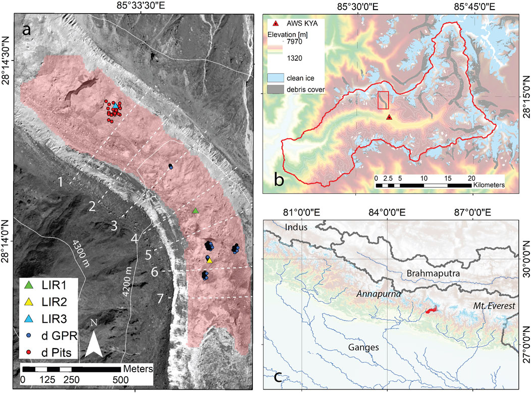
FIGURE 1. (A) Overview map of the study site, showing the ablation tongue with the locations of atmospheric measurements (LIR1, LIR2, LIR3) as well as debris thickness measurements by GPR (d GPR) and excavation (d Pits). The red shaded area shows the model domain in 2013, where mass loss measurements are available. The image shows the part of the tongue where continuous debris is observed. The white dashed lines show the flux gates (used for the calculation of emergence velocity (see Supplementary Material). (B) Langtang catchment, with all debris-covered glaciers shaded grey, and the location of the Kyanjing AWS (AWS KYA) south of Lirung Glacier. (C) Location of Langtang catchment in the Central Himalaya.

Climate Data

Meteorological measurements are available from an automatic weather station (AWS) installed on the glacier for multiple years (LIR1, 28.2349°N, 85.5613°E, 4,195 m; LIR2, 28.2326°N, 85.5621°E, 4,075 m; LIR3, 28.2396°N, 85.5571°E, 4,200 m) as well as from an off-glacier location (Kyanjing, 28.2108°N, 85.5695°E, 3,862 m, Figure 1B). All sensor specifications are shown in Table 1 and measurement periods in the Supplementary Table S1. The locations of measurements are marked in Figure 1A. The surface temperature of the debris at the AWS location was derived from outgoing longwave radiation, assuming a debris emissivity of 1.

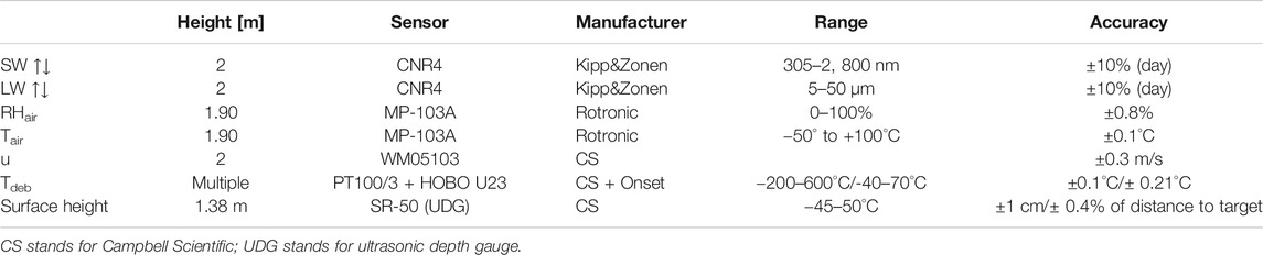
TABLE 1. Sensor specifications for the AWS off-glacier (Kyanjing) and on-glacier locations. Climate data at LIR3, used to validate the usability of off-glacier climate data, were collected with a WS500-UMB.

Debris Data

Debris thickness measurements of Lirung Glacier are available from ground-penetrating radar (GPR) measurements in 2015 (McCarthy et al., 2017), as well as from 27 pit measurements between 2016 and 2017 (Figure 1A). These measurements are aggregated to the model resolution (10 m) and used to validate the debris thickness estimate.

Measurements of debris temperatures are available from all three locations on Lirung Glacier, covering varying depths. Debris densities, porosity and volumetric soil moisture were measured by taking 55 samples at varying depths in the 27 pits in October 2016 and April 2017. Samples were taken with a 100 ml soil corer for the fine textured layers and were dried for 24 h and weighed and sieved in the lab.

Unmanned Aerial Vehicle Data

Elevation data of both glacier tongues are obtained from co-registered orthomosaics (0.1 m resolution) and DEMs (0.2 m) derived from multiple UAV flights with an optical camera (Supplementary Table S1). The DEMs were resampled to 10 m resolution and corrected for flow. From the same flights, velocities were derived which, in combination with modeled ice thickness, were used to compute emergence velocities over the glacier tongue (see Section 2 in Supplementary Material). We refer to previous studies on the generation of DEMs and velocity products (Immerzeel, et al., 2014a; Kraaijenbrink, et al., 2016b).

Methods

Mass Loss Data

We derived mass loss by comparing the DEMs of two consecutive timesteps that were corrected for horizonal flow and the emergence velocity. To correct for emergence velocity, we placed fluxgates perpendicular to the flowline at approximately 500 m distance (Figure 1) and used modeled ice thickness data (Farinotti et al., 2019) and UAV-derived flow velocities, determined similarly as in Kraaijenbrink et al. (2016a). We then calculate emergence velocities for the resulting segments and correct the mass loss product accordingly. Average emergence over the model time period in 2013 is estimated to be small (approximately 0.07 m averaged over the model domain over the 157 days, see Supplementary Table S2). Using the individual DEM uncertainties (0.25 m, Immerzeel et al., 2014a; Kraaijenbrink and Immerzeel, 2020) we estimate the uncertainty of the mass loss product to be 0.35 m.

Debris Thickness

Deriving debris thickness in space is challenging and several studies have attempted this at the glacier scale. Foster et al. (2012) initially proposed to derive thickness from thermal imagery, following the logic that the energy absorption by the glacier ice underneath would be reflected more in the surface temperature of a thin than of a thick debris layer. Some studies build on this approach (Rounce and McKinney 2014; Schauwecker et al., 2015; Kraaijenbrink et al., 2017) but little validation data exists and uncertainties remain large, because the signal saturates at thicknesses over ∼30 cm and other factors drive the surface temperature variation, e.g., shading, moisture and spatial variation in surface energy balance components. Secondly, Rounce et al. (2018) used the inversion of an energy balance model to derive debris thickness. Finally, it is also possible to use observed mass loss data and invert the Østrem curve (Rounce et al., 2018). While both latter approaches show promising results, inverting the Østrem curve is considerably less computationally intensive and is used in this study (Eq. 1). As we perform this analysis using mass loss data from 2016, while we apply the energy balance model in 2013, we are able to produce an independent debris thickness map. To create an average Østrem curve we use data from all currently published studies that include both debris thickness as well as melt rates. The following equation is solved at each individual pixel:

where d is the debris thickness [m], $\dot{m}$is the UAV-derived melt rate [m yr⁻¹], m_c is the melt rate [m yr⁻¹] at critical thickness (2 cm) over the same period as the mass balance was derived and a [m⁻¹] and b [−] are parameters. While both the critical thickness and m_c can in reality be expected to vary over the glacier, we chose to calculate m_c with the measured fluxes at the AWS for the fixed critical thickness, in order to avoid introducing unquantifiable errors into our procedure. Running 100 simulations only varying parameters within their uncertainty (see Section Debris Properties and Conductivity) results in m_c = 0.04 m d⁻¹ (σ = 0.01 m d⁻¹).

Using velocity and emergence-corrected mass balance data for the monsoon season 2016, in conjunction with the mean Østrem curve, we then derive a distributed map of debris thickness. While strictly speaking this debris thickness map only applies for a specific time step, we argue that due to the low surface velocities of Lirung Glacier (with maxima of ∼2 m a⁻¹) and the resolution of the model (10 m) it is reasonable to apply it ± 3 years from the date of acquisition.

Energy Balance Model

The sub-debris melt model is based on earlier work by Reid and Brock (2010), which numerically estimates the surface temperature of the debris by considering the balance of the heat fluxes at the air-debris interface and melt is calculated by heat conduction through the debris. One advantage of this approach is that it does not require surface temperature as an input, a variable that is notoriously difficult to obtain accurately in space (Steiner and Pellicciotti 2016; Kraaijenbrink et al., 2018). The energy balance $F\left(T_S\right)$at the air-debris interface can be written as

where T_s is the surface temperature, SW↓↑ is the incoming and outgoing shortwave radiation, LW↓↑ is the incoming and outgoing longwave radiation, H and LE are sensible and latent heat flux respectively and G is the ground heat flux through the debris. We ignore fluxes from precipitation in this work, as on-glacier measurements do not exist and the fluxes are often considered negligible.

We then solve T_s using a Newton-Raphson scheme

where $F\mathrm{’}\left(T_S\right)$, the derivative of the total surface flux, is calculated by the central difference method. The initial estimate for $T_S(n=0)$, is always chosen as the air temperature $T_{air}$, and Eq. 2 is subsequently iterated until $T_S\left(n+1\right)- T_S\left(n\right)<0.01$. Iterations are stopped when n reaches 100 or if the temperature gradient in the topmost debris layer exceeds 5°C cm⁻¹. This is rarely the case but ensures that the surface does not heat up to unrealistic values, which would drive sensible heat and outgoing longwave radiation fluxes to unrealistic levels.

Incoming solar radiation $SW\downarrow$ is taken from measurements and corrected for local topographic shading using the initial DEM. Shading is calculated following the approach in Buri et al. (2016b) in which the view factor is calculated, i.e. the fraction of the sky blocked by surrounding topography is calculated. Considering the actual view factor at the AWS where radiation is measured, the $SW\downarrow$is corrected using the cell-specific view factor. Outgoing shortwave radiation $SW\uparrow$ is computed using a constant albedo ${\alpha }_d$ determined from on-glacier measurements. Incoming longwave radiation $LW\downarrow$ is taken from measurements wherever available and otherwise computed using a model developed for the Himalaya (Kok et al., 2019). Contrary to the original model, which used stability corrections based on the Richardson number, we calculate sensible and latent heat flux only using a bulk transfer coefficient (Nicholson and Benn 2006; Cuffey and Paterson 2010), which was found to be more appropriate compared to direct measurements of turbulent fluxes (Steiner et al., 2018). Since the specific humidity of the debris surface is not known, and will remain difficult to derive in space and time, it is derived based on a relation with surface temperature (Steiner et al., 2018).

Debris Properties and Conductivity

The conduction from the air-debris to the debris-ice interface can be calculated from a heat-conservation equation based on Fourier’s law with the partial derivatives of temperature $T_{i,s}$

where i denotes time t, and s denotes depth z, and ${\rho }_d$, $c_d$, and $k_d$ are density, specific heat capacity and thermal conductivity of the debris, respectively, all assumed to be constant with depth and over time. The equation is solved numerically by dividing the debris layer in N layers of 1 cm each and taking the surface temperature $T_s$ and the ice temperature $T_i$ as boundary conditions. For cases where the debris layer is thinner than 5 cm, the number of layers is fixed to 5. For a full description of the numerical solution see (Reid and Brock 2010).

The effective thermal conductivity of debris is calculated using the density of the debris pack

where $\kappa$ [m² s⁻¹], is the apparent thermal diffusivity determined from profiles of debris temperature collected at multiple sites and times, following the same approach as described in (Conway and Rasmussen 2000). We only use measurements during the night (20:00 to 07:00) to avoid inversions. ${\rho }_r$ is the density of the actual rock making up the debris [2,650 kg m⁻³, considering the region mainly consists of metamorphic gneiss (Macfarlane et al., 1992)], $c_r$ is the specific heat capacity of rock (890 J kg⁻¹K⁻¹) and ${\varphi }_d$ is the debris porosity, which we determine from field measurements [−]. ${\rho }_{w/a}$ are density, and $c_{w/a}$the specific heat capacity of water and air, respectively. $\theta$ is the soil moisture [m³ m⁻³]. The second term of the equation describes the conductivity through the space between the debris, and can be set to fully saturated ($\theta$=${\theta }_{sat}$ = 0.2) or completely dry ($\theta =0$). As moisture changes in space, depth and time, it likely is the biggest driver of uncertainty for calculated conductivity.

To characterize the debris properties in depth we also determined the grain size distribution for 30 samples from different depths at the 27 pit sites around LIR3. These samples exclude rocks larger than 5 cm.

Uncertainty due to spatial and temporal variability in all of the parameters associated to the debris, most importantly the thermal conductivity, are accounted for by a Monte Carlo simulation in which multiple realizations of the model with random combinations of the input parameters are performed. The parameter space and distribution type are based on field data. All parameters and their ranges used in this study are detailed in Table 2. To assess the ability of the model to reproduce mass loss accurately we run a number of simulations. First, the model is run at the location of the AWS where climate data and debris thickness are well constrained and we only vary debris thermal conductivity (which is dependent on porosity, soil moisture and diffusivity), debris density and surface roughness using 1,000 random parameter sets. Secondly, for 64 locations where debris thickness has been measured 1,000 simulations are run where, in addition, debris albedo, air temperature, relative humidity of the air, wind speed and incoming longwave radiation are varied within the expected range of uncertainty. This allows us to discuss the sensitivity of the energy balance model to these variables and constrains the number of model runs required for all pixels to just 50 realizations by only varying debris thermal conductivity. Although the model is coded to run in parallel, performing 1,000 realisations on each individual pixel for Lirung Glacier for one melt season would take >2 weeks to execute on eight cores, so increasing the computational efficiency by reducing the parameter space is a helpful way forward for multi-annual and regional applications.

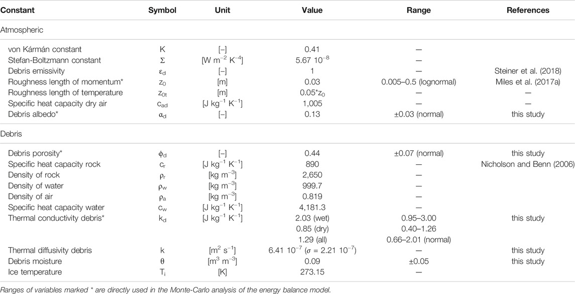
TABLE 2. Constants used in the study and the range used for the uncertainty analysis.

Index Models

A variety of index models are used in literature to calculate melt on clean ice glaciers, most commonly relying on air temperature only (Hock 1999), i.e., a temperature index model, and occasionally also considering incoming solar radiation (Pellicciotti et al., 2005), i.e., an enhanced temperature index model. The latter approach was adapted for a debris-covered glacier (Carenzo et al., 2016) and this approach has also been applied on Lirung Glacier in a catchment scale study (Ragettli et al., 2015). As energy balance studies are generally computationally more expensive and rely on more input data, we compare both approaches and test the model performance when only using data from an off-glacier station. In the simpler temperature index model, melt m [mm w.e. h⁻¹] is calculated as

where T_air [°C] is the air temperature at time t−lag_T*d, where d [m] is debris thickness and lag_T [h m⁻¹] is the time per unit distance it takes for the energy flux to travel through the debris pack. TF is the temperature factor calculated as

with TF₁ and TF₂ being two free parameters to be calibrated.

To test the suitability of the model proposed in Carenzo et al. (2016), we also use

where SRF is the radiation factor computed as $SR{F}_1 {\text{e}}^{SR{F}_{2}d}$, with SRF₁ and SRF₂ being two additional free parameters. $SW\downarrow$ [W m⁻²] is incoming solar radiation, $\alpha$ [−] albedo of debris and lag_SW the time lag as described above. We refer to the two equations as dTI (for the temperature index model) and dETI (for the enhanced model) respectively.

Results and Discussion

Debris Properties

Debris composition is very variable across the glacier and with depth. Surface cover ranges from loose boulders to sandy patches and the surface properties do not necessarily indicate a vertical consistency in debris texture (Figure 2). There is a tendency for debris to become finer towards the ice (Figure 2F, Naylor, 1980). In some pits (Figures 2C,E) a water table of ∼5 cm above the ice, with a very weak current of melt water with suspended sediments, was observed. Reworking by ice flow, slumping of debris due to collapsing cliffs and channels (Benn et al., 2012; Buri et al., 2016a; Miles et al., 2017b) and deposition of material eroded from the surrounding moraines (Woerkom et al., 2019) continuously alters the composition. We use point scale observations over limited periods of time to derive a reasonable range of debris thickness and debris conductivity used in the model.

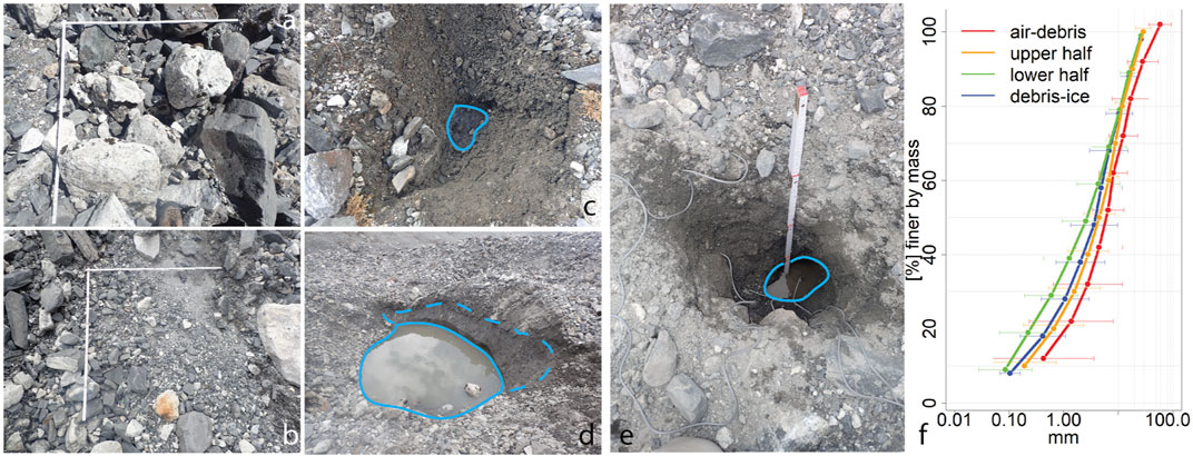
FIGURE 2. (A) A typically coarse surface with little change between years and likely thick cover underneath, (B) example of short-length-scale transition between cobbles and sand. White ruler shows a 1 by 1 m area. (C) Surface with thin debris cover (∼0.15 m) consisting of fine material, where melt water is surfacing (solid blue line). (D) Glacier ice (dashed blue line) appearing in a region of otherwise thick cover, with multiple pits in a 10 m radius of >1 m depth. (E) Melt water ponding in a deep pit (∼0.65 m). (F) Grain size distribution of the debris pack, with samples from the debris surface, inside the debris pack (upper and lower half) and from just above the ice plotted separately.

Debris thickness measurements derived from GPR (McCarthy et al., 2017) and debris pits, although measured at different locations, exhibit similar mean values (0.84 and 0.82 m respectively) with minimum depths at 0.11 and 0.4 m and maximum depths at 2.3 and 1.6 m, respectively. Both distributions show a log-normal distribution, corresponding to observations of thickness on other glaciers (see Nicholson et al., 2018). Hence, for the Monte Carlo runs, we use a set of debris thicknesses that are sampled from a log-normal distribution, with a mean of 0.84 m and minimum and maximum values of 0 m and 2.7 m respectively, based on the GPR measurements.

To produce a distributed debris thickness map, we produced standardized Østrem curves from all available studies that show field measurements of ablation and debris thickness (Figure 3A). Assuming a critical thickness, where melt below debris is equal to bare ice melt, these curves derived in different climates can be compared. This still leaves a considerable spread, especially as the debris thickens.

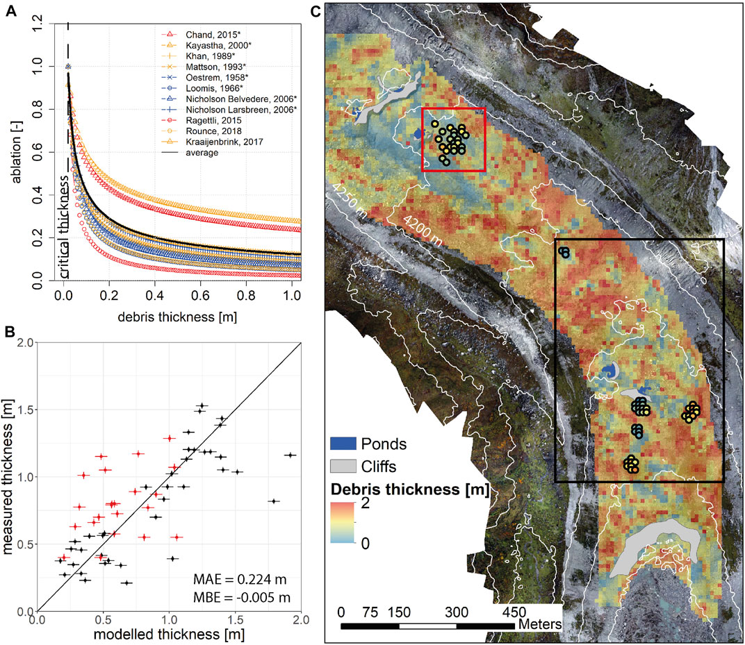
FIGURE 3. (A) Standardized Østrem curves for all studies with field data (*) and three modeling studies. Only data from field studies was used to generate the average curve. The vertical dashed line shows the critical thickness, where melt is equal to a clean ice glacier in the same climate (2 cm). In red are studies from Lirung Glacier, yellow are from HMA, blue are studies from other regions. (B) Modeled compared to measured debris thickness at 10 m resolution, red are from pits and black from GPR measurements as noted by the squares in (C). (C) Modeled debris thickness map. Points shown in the black frame are from GPR measurements, red frame denotes excavated pits.

The calibrated parameters for Eq. 1 are a = 0.13 (σ = 0.002), and b = -0.52 (σ = 0.006), which is very similar to the curve used in Kraaijenbrink et al. (2017) that used a similar approach and data (including thermal Landsat bands, a = 0.11 and b = −0.51), but considerably different from two other studies that used a similar inversion but were based on local data (Ragettli et al., 2015; Rounce et al., 2018). The distributed map was produced using the difference between the DEMs in May and October 2016, corrected for emergence and aggregated to a 10 m product. All melt features not covered by debris (cliffs and ponds) as well as outliers (beyond the 5th and 95th percentile) were removed, so were pixels where mass loss was below the accuracy of the product (0.35 m) as well as individual pixels before aggregation that were thicker than 2 m. While thicknesses beyond 2 m may occur, just 0.5% of ∼6,000 GPR data points and none of the pits are this deep. When aggregated to a 10 m resolution thicknesses over 2 m are hence even less likely. We then derived the thickness for the remaining pixels and interpolated over the complete domain by inverse distance weighted interpolation. Comparing the resulting map (Figure 3C) to point measurements (Figure 3B), shows an overall agreement, with no bias and an acceptable mean absolute error (MAE) of 22 cm. Debris thickness is generally thicker closer to the moraines due to a constant resupply from the moraines (Woerkom et al., 2019). It is especially thin at the terminus where bare ice appears as the tongue retreats rapidly, thickens in the lower part but thins again towards the accumulation are where it then gradually transcends into the bare ice area (Figure 3C). Most challenging however is that variability over relatively short length scales is high and can happen gradually or abruptly, with thickness differences in the range of 1 m over horizontal distances of 100 m on both Lirung Glacier and other field sites (see Table 2 in Nicholson et al., 2018). The uncertainty for individual pixels from the model logically remains considerable and is a result of the spread in the Østrem curves, the critical debris thickness and the uncertainty of the DEMs.

Measurements of debris temperatures at different locations and different depths provide largely similar results (Figure 4), suggesting that diffusivity through the debris is relatively constant in space even with differences in debris texture. Generally, temperatures are higher in the wet season, with the exception of 2013, where surface temperatures were in general higher but also sensors malfunctioned towards the end of the wet season. As a result, most data from the dry season in this year is from pre-monsoon, which is generally warmer. Measurements in the uppermost part of the debris pack also suggest that most of the diurnal variability is attenuated after 10 cm of debris. The mean peak temperature pattern at the top and bottom profiles of all years reveals that the transit time of the temperature peak is roughly similar in all profiles, ranging from 15.6 h m⁻¹ in the wet season at LIR2 to 18.5 h m⁻¹ in the wet season at LIR3.

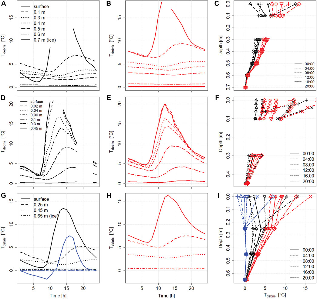
FIGURE 4. Temperature profiles in debris measured at the AWS in 2012 [(A–C), LIR1], 2013 [(D–F), LIR2] and from 2017 [(G–I), LIR3]. Blue is the winter season (1st January to 28th February), red the wet season (06/15 to 09/19) and black the dry seasons.

From the temperature profiles we can calculate diffusivity in the wet (7.4 × 10⁻⁷ m² s⁻¹) and dry season (6.8 × 10⁻⁷ m² s⁻¹). This is similar to the values from Conway and Rasmussen (2000) (6 and 9 × 10⁻⁷ m² s⁻¹) and Nicholson and Benn (2013) (9.5 × 10⁻⁷ m² s⁻¹ in the wet summer and 7 × 10⁻⁷ m² s⁻¹ in winter) but much higher than values measured on likely drier surroundings in the range of 3–3.9 × 10⁻⁷ m² s⁻¹ (Nicholson and Benn 2006; Juen et al., 2013). Recent investigations in the Everest region show similar gradients of temperature through the debris, suggesting that these profiles remain relatively stable throughout the season (Rowan et al., 2020). This space and time invariance provides some confidence in applying constant diffusivity values in distributed analysis.

Since the debris is never completely dry, its moisture content needs to be accounted for in the determination of thermal conductivity. Soil moisture measurements in a number of pits indicate a moisture content of 0.01–0.2 m³ m⁻³ (μ = 0.09, σ = 0.05), where the maximum value corresponds to saturation of sandy soils. Highest variability can be found near the surface, due to its very variable composition (Figures 2, 5A). The general distribution corresponds to typical soil moisture curves (e.g. Genuchten, 1980), with the peculiar case here that soil moisture at the bottom of the debris layer is higher due to melting ice, while close to the surface it is due to precipitation and condensation. Measured porosity on the glacier ranged from 0.30 to 0.59 (μ = 0.44, σ = 0.07), which corresponds to the only other two measurements from literature, namely a mean of 0.43 in Popovnin and Rozova, (2002) and a range between 0.19 and 0.6 in Collier et al. (2014). The actual debris density was between 1,300 and 1,950 kg m⁻³ (μ = 1,588 kg m⁻³, σ = 175 kg m⁻³), which corresponds well to the mean of 1,496 kg m⁻³ used in Reid and Brock (2010). Considering the large variability in space and depth, we use all diffusivity estimates and moisture data from literature and from this study to aggregate a reasonable range of conductivity for the model, shown as boxplots in Figure 5B. Note how assuming full saturation or complete dryness results in a very large range of conductivity values. The median conductivity of 1.29 J m⁻¹ K⁻¹ matches well with the few available direct measurements from our field site. Reported conductivity values are rare for specific seasons (Nicholson and Benn 2006; Nicholson and Benn 2013), but do exist for unspecified conditions (Conway and Rasmussen 2000; Reid and Brock 2010; Juen et al., 2013; Rounce et al., 2015). These reported values correspond well with the range in conductivity values that we have derived (Figure 5B).

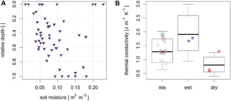
FIGURE 5. (A) Soil moisture measurements from pits around LIR3. (B) Thermal conductivity calculated using temperature profiles and the moisture content. The box plots indicate the range of thermal conductivities as calculated using the range of diffusivities from literature and using the observed moisture range (mix), full saturation (wet) and completely dry debris assumptions (dry). Solid dots are values from literature, transparent crossed dots are calculated with diffusivity and debris moisture only from the observed field data (red—dry, blue—wet).

Two main observations can be made from the grain size distribution (Figure 2F). First, the variability with depth is quite large, with finer sediments being more abundant in the lower part of the debris pack. Approximately 40% of the debris is sand, which results in a relatively high water retention capacity compared to gravel or small boulders. This results in an increase in conductivity compared to a drier coarse-texture debris pack by a factor of 2 (Figure 4B). Such considerations are essential to further drive development of more complex models that are able to incorporate moisture (Collier et al., 2014; Giese et al., 2020), but also for routing times of melt water from the glacier as melt water does not immediately become available to discharge. Second, due to this available water in the pores and relatively dense debris texture, the debris pack is largely frozen below a depth of 20 cm in winter. On Lirung Glacier this occurs specifically in winter (Figure 4). As temperatures become positive in spring at the surface, it takes up to a week to defrost the entire debris pack at depths of ∼1 m. Although we can calculate the available energy for (re-)freezing our model cannot account for lateral or vertical transport of water within the debris and hence an appropriate quantification is impossible. However, melt estimates for the cold season are likely to overestimate actual rates, especially in spring, when this process is unaccounted for.

Climate Data and Resulting Uncertainties

Due to the heterogeneity of the debris surface, climate variables vary over the surface and errors are introduced due to the lapsing of variables from the location of weather stations to other parts of the glacier. By comparing climate data from three locations on the glacier, we assess the extent of this variability (Figure 6).

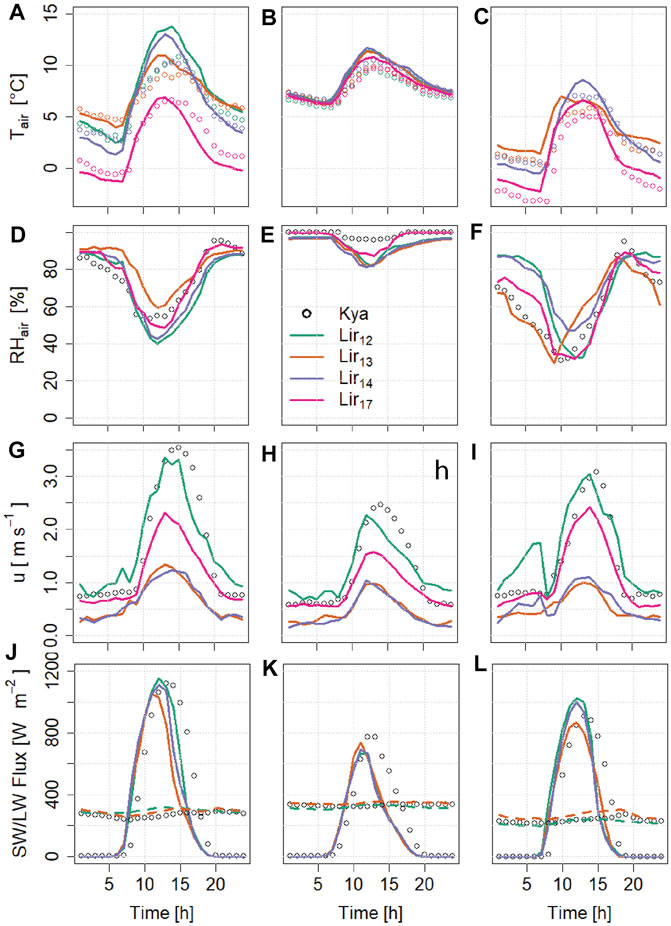
FIGURE 6. Mean diurnal cycles for climate variables used in the energy balance, including air temperature (A–C), relative humidity of the air (D–F), wind speed (G–I) and incoming shortwave (solid lines) and longwave radiation (dashed lines, (J–L)). For air temperature the lapsed data from Kyanjing (Kya) to the respective on-glacier location is shown. Wind speed at Kyanjing is shown with a factor of 0.5. The three columns represent three seasons, pre-monsoon, monsoon and post-monsoon from left to right. Lir_12-17 refers to the AWS on Lirung Glacier. Lir₁₇ was operational from September 2016 to October 2018, while all other setups only measured during the monsoon in the respective year (see Supplementary Table S1 for exact periods).

Variability in air temperature over debris cover was investigated for Lirung Glacier in earlier studies (Fujita and Sakai 2000; Steiner and Pellicciotti 2016). To evaluate the use of off-glacier measurements, we used a seasonally varying lapse rate (Heynen et al., 2016) up to the glacier snout combined with lapse rates for the glacier surface for the specific seasons (−0.005, −0.0066, and −0.0078°C m⁻¹ for pre-monsoon, monsoon and post-monsoon respectively, Steiner and Pellicciotti, 2016). Lapsing temperature from an off-glacier station introduces an additional error on top of the spatial variability (Figure 6), resulting in a mean bias error (MBE) between 1 and 2°C. This is especially visible during the day and larger during the monsoon. We therefore use a conservative uncertainty range of 2°C for all air temperature values. This is especially relevant when using simpler index models that only rely on air temperature as a proxy for melt. The fact that we are able to reproduce air temperature reasonably well using this lapsing approach provides confidence in the use of a single AWS for deriving melt rates for multiple glaciers in a catchment.

While relative humidity also changes with elevation, the trend is less clear and variability is more impacted by local debris properties (Bonekamp et al., 2020). However, no measurements at different locations are available over the same period. Measurements at the off-glacier station are similar to on-glacier measurements with the exception of the monsoon season, in which the air is much more humid off-glacier at the Kyanjing station in the main valley. The root mean square error (RMSE) ranges between 10 and 20%. We use a conservative uncertainty estimate of 20% for the modeling.

Wind speed is also variable over the debris surface due to the hummocky terrain, but is approximately a factor 2 lower than at the off-glacier AWS, which is located in the exposed main valley (Figures 1B, 6). While in 2012 and 2017 the AWSs were located on relatively exposed parts of the glacier, the station was situated in a depression from 2013 to 2014, resulting in a decrease of average wind speed by a factor of 3, which significantly affects the turbulent fluxes (Steiner et al., 2018). When using the on-glacier data from 2013 to drive the model, we allow wind speeds to vary by up to a factor of 2.5 to account for this variability.

Finally, incoming radiation is affected by the hummocky terrain as well. It causes parts of the surface to be shaded longer than more exposed sections and hence receive less direct incoming shortwave and longwave radiation. These sites also receive added longwave radiation from the surrounding debris. We apply the sky view factor relative to the location of the measurement of radiation for all pixels when running the energy balance. For the sensitivity analysis, we furthermore assume that the longwave radiation flux may vary by ± 50 W m⁻² due to additional radiation emitted by the surrounding debris.

Albedo is relatively consistent between the 3 different locations on the glacier, with daily mean values between 0.12 and 0.16 during the dry seasons and values down to 0.06 on rainy days in the monsoon season, when debris is wet. The mean albedo ranges between 0.11 in 2012 and 0.13 in all other years. We therefore use a normal distribution with μ = 0.13 and the measured σ = 0.03 for the uncertainty analysis.

Energy Balance Model on the Point Scale

At the location of the AWS the energy balance can be validated accurately in 2013 as the climate data is available at that specific site and the surface elevation changes are continuously monitored during the first month. It also allows us to validate the performance of the model against measured surface temperature. Figure 7A shows modeled and measured mass loss at the location of the AWS. The modeled debris thickness for this location is 0.37 m, which corresponds to the 0.29 m measured at the location of the AWS and 0.45 m measured in another pit just 3 m away. This variability within a relatively small area is indicative of the spatial heterogeneity of debris thickness (Anderson and Anderson 2018; Nicholson et al., 2018).

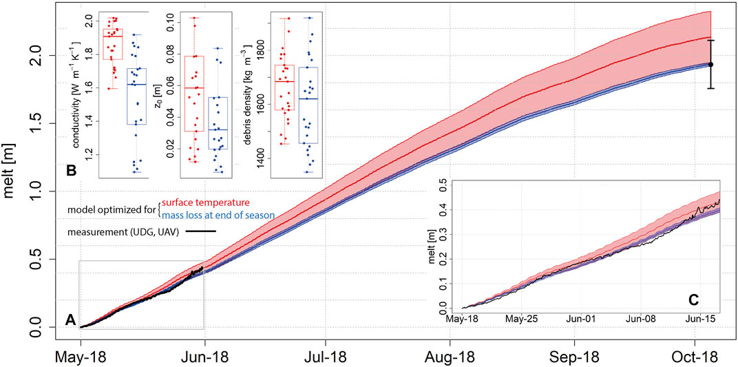
FIGURE 7. (A) Modeled melt at the location of the AWS in 2013. The blue and red line and shaded area show the mean and standard deviation of the 25 best performing model runs (97.5th percentile) compared to the observed mass loss from the UAV and the observed surface temperature respectively. The error bar of the UAV measurement corresponds to the uncertainty of the DEM accuracy. The solid black line are hourly measurements from an ultrasonic depth gauge (UDG, Table 1), which only monitored for a limited time, shown in detail in (C). (B) Conductivity, surface roughness and debris density for the 25 best performing model runs, once for optimization with UAV (blue) and once with surface temperature (red).

In Figure 7 we focus on the 25 model runs of 1,000 simulations that match observed mass loss (blue) or observed surface temperature (red) most closely. For surface temperature this was assessed by finding the time series that had the lowest combined MBE and RMSE and highest NSE. It is encouraging however, that the model also matches well with the independent measurement of surface height at the beginning of the season (Figure 7C). Unfortunately, the sensor also tends to tilt as debris moves which eventually caused it to fall over after June. Figure 7B shows the spread of the model parameters for the best performing runs. The range for conductivity values is large and the values are quite high, with an average of 1.6 W m⁻¹ K⁻¹. The mean surface roughness value corresponds well with the observations from the very same location in 2014 (0.03 m) (Miles et al., 2017a). The model is relatively insensitive to debris density (Figure 7B).

Alternatively, model performance can also be assessed by comparing the modeled and measured surface temperature, which allows for an assessment of the model performance over time (Reid and Brock 2010). This works well for the AWS location, indicated by a mean Nash-Sutcliffe Efficiency (NSE) of 0.79 and a RMSE/MBE of 3.6°C/−0.4°C for the 25 best performing runs. While this approach is useful to evaluate the ability of the model to reproduce fluxes accurately, it depends on the accuracy of the surface temperature measurements (Steiner and Pellicciotti 2016; Kraaijenbrink et al., 2018). The results presented here suggest that using either surface temperature or a single mass loss measurement as validation provides similar results. However, the model runs that correspond most closely to the surface temperature measurements overestimate the final mass loss (Figure 7A), the measurement from the local sensor (Figure 7C) and also tends to be on the upper end of resulting conductivity values (Figure 7B).

Irrespective of whether mass loss or surface temperatures are used for validation, the modeled surface temperatures agree well with the observed temperatures (NSE = 0.76/0.77, MBE = −0.2/1.1°C, Figure 8). However, the model fails to capture the very high peaks of surface temperature (>35°C) and overestimates temperatures on days when the observed values suddenly drop due to overcast conditions.

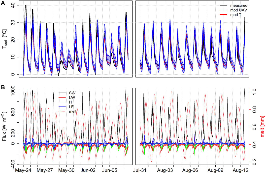
FIGURE 8. Measured and modeled surface temperature of the debris at the AWS, with ‘mod UAV’ denoting the results that fit best with the UAV mass loss measurement and ‘mod T’ those fitting best with observed surface temperature (A). Resulting (net) fluxes and melt rates based on the model (B). The shaded area shows the range of results based on the 25 best performing model runs after comparison of the modeled mass loss with the measured mass loss (Figure 7).

The net shortwave, longwave, latent and sensible heat fluxes are shown in Figure 8. Net shortwave radiation is the dominant flux. Net longwave radiation is consistently negative on clear days but becomes positive on overcast days. The sensible heat flux is consistently negative, while the latent heat flux is generally low and can be negative or positive. Modeled melt lags the energy peak by a couple of hours due to the delay of energy transfer through the debris. As a result, sub-debris ice also melts, when the surface energy balance is negative. This is in contrast to clean ice glaciers, where melt stops as soon as the net energy is below zero.

Energy Balance on the Distributed Scale

As a first step we applied the energy balance on all pixels where debris thickness observations were available (Figure 9). We selected the 25 simulations from the total of 1,000 that reproduced observed mass loss best. It is clear that the highest mass loss is observed for thin debris as expected. However, below half a meter of thickness there is a lot of variability in mass loss, as other drivers, such as moisture and debris texture become more important. Nevertheless, the model is able to reproduce the observed mass loss in nearly all cases, which indicates that all essential processes are incorporated.

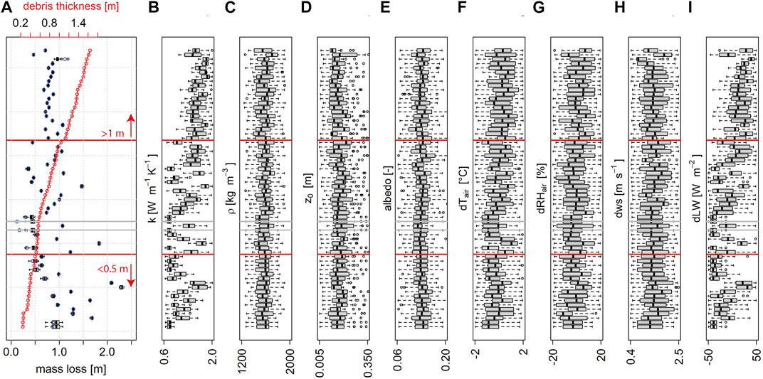
FIGURE 9. (A) Modeled mass loss at locations where debris thickness observations are available. The boxplots cover the 25 model runs that most closely reproduce observed mass loss. (B–I) Range of variables (from left to right: debris conductivity, debris density, surface roughness, surface albedo, as well as uncertainty/spatial variability ranges for air temperature, relative humidity of air, wind speed and incoming longwave radiation from surrounding terrain). Grey solid horizontal lines show cases where the observed melt could not be reproduced with any parameter combination.

The model is sensitive to all the parameters that were varied during the Monte Carlo runs, indicated by a relatively narrow range around the respective median (Figure 9). However, for debris density, surface albedo and surface roughness the optimal values are independent of debris thickness and therefore a constant value for all pixels can be assumed for these variables.

Of the climate variables the model is most sensitive to the potential variability in space and time of longwave radiation and slightly less sensitive to air temperature. Both these variables increase with increasing debris thickness. Relative humidity and wind speed on the other hand show no such trend and the observed value from a single location provides satisfactory results on the glacier scale.

Incoming longwave radiation from surrounding terrain plays a role since it directly adds energy to the surface. However, quantifying spatial patterns of longwave radiation on a hummocky surface is challenging. The uncertainty in observed surface temperatures (Kraaijenbrink et al., 2018) makes it even more difficult to quantify additional incoming longwave radiation in space.

For the fully distributed model, we only run 50 simulations per pixel in which we allow k_d to vary, the variable to which the model is particularly sensitive (Figure 9). Using constant parameters but a variable k_d, we model mass loss in space. We include pixels where melt was observed and where no cliffs or ponds were present at the beginning of the season.

Figure 10A shows the difference between observed and modeled melt, applying varying k_d values that fit most closely to the observed data. The blue and green boxplots in Figure 10C show the results aggregated for 100 m bins in distance from the terminus. The mean observed melt over the whole domain is 0.89 m (±0.76 m). Modeled melt using spatially variable conductivity is 0.77 m (±0.37 m) and using fixed conductivity is 0.88 m (±0.42 m). Observed high values cannot be reproduced by the model, which can be explained by mechanical processes of mass loss, i.e. slumping around cliffs and ponds as well as disintegration of subglacial structures. The high retreat rates at the terminus, where debris cover is present but thin and ice repeatedly collapses, are equally poorly represented. However, overall it is possible to reproduce observed melt rates well, with a RMSE and MBE of 0.29 and 0.04 cm d⁻¹ respectively. The resulting k_d map (Figure 10A, inset) naturally follows melt patterns. Where melt is high but debris thick and surface features like cliffs and ponds are rare, k_d is high. Where melt is low, in this case the middle section of the tongue, very low k_d counter balances the energy input at the surface. Rather than reflecting actual k_d, the value here acts as a free parameter. However, these values do not only lie within the range of previously reported values for conductivity, they also have some physical merit. Thick and continuous debris can hold more moisture leading in turn to higher bulk k_d values. In the center part and the upper part of the modeled domain, debris is discontinuous and relatively thin, making the debris pack more susceptible to evaporative drying and drainage and hence decreasing the conductivity.

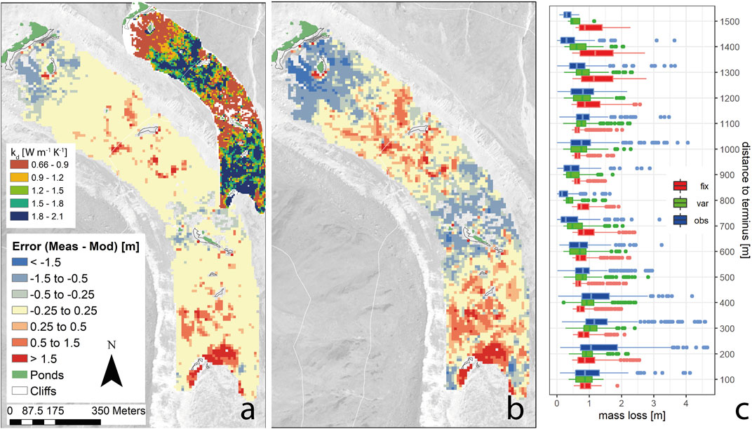
FIGURE 10. (A) Difference between observed and modeled melt with variable (shown as an inset) and (B) constant conductivity k_d. (C) Melt over all pixels for the observed (obs), variable k_d (var) and fixed k_d (fix) case, binned in distance to the terminus.

Distributed data of conductivity is however virtually impossible to retrieve, let alone accounting for its change in time. For practical applications, we need to assume a constant conductivity value in space and time. Figure 10B shows the results for the median k_d of 1.41 W m⁻¹ K⁻¹. Results become less variable and as a result modeled rates in the central part are considerably higher than observed. This is notably also where observed mass loss was especially low even though a number of cliffs and ponds were present and emergence velocities are possibly higher than what we estimated. The RMSE increases subsequently to 0.47 cm d⁻¹ but MBE remains low (−0.03 cm d⁻¹).

With the model we compute melt for all ∼4,500 pixels of the debris-covered area of the glacier with a timestep of 1 h. In Figure 11 the average melt rate below 0.5 m, between 0.5 and 1 m and above 1 m debris thickness is shown. Melt rates clearly follow the air temperature and solar radiation, albeit with a considerable lag (Figure 11B). Even for locations with debris thinner than 0.5 m, the melt peaks a few hours after the temperature peak. Three specific processes illustrate the effect of climatic drivers on temporal melt patterns below debris. Firstly, when there are a number of subsequent cloudy days with limited shortwave radiation (e.g. during the first half of July, Figure 11A), melt rates overall remain unaffected, however melt rates during the night under thinner debris surprisingly increase. This can be explained by the absence of radiative cooling during the night and the higher longwave radiation input from clouds. This results in a less negative or even positive net longwave radiation without a clear diurnal cycle (see May 30th in Figure 8). While the increase of longwave radiation seems small, it consistently increases the entire day, while the decrease of solar radiation only occurs during daytime. In addition, turbulent fluxes become less negative as radiative heating decreases (Steiner et al., 2018). Secondly, when air temperature and shortwave radiation decrease (Figure 11B) melt rates decrease everywhere, resulting in an overall decrease of meltwater output on the glacier scale. Thirdly, in the beginning of September the solar radiation remains consistently high and the daytime temperatures are similar to the monsoon. However due to the strong radiative cooling at night, temperatures drop considerably causing a decrease in melt. Nighttime temperatures therefore have an important effect on melt below debris.

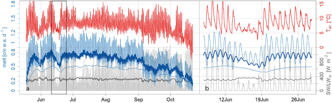
FIGURE 11. (A) Mean hourly melt rates during the model period melt below average debris thickness (50–100 cm, thick dark blue line) as well as thick (>1 m) and thin (<0.5 m, thin light blue lines below and above). Additionally shown measured air temperature (red), incoming shortwave radiation (light grey) and incoming longwave radiation (dark grey). The black rectangle in panel a shows the boundaries of the inset of panel (B).

We conclude that air temperature is a good indicator of both variability and magnitude of sub-debris melt rates in a monsoon climate, due to the interplay between shortwave radiation, longwave radiation and turbulent fluxes in the energy budget.

Sources of Uncertainty and Model Limitations

There remain several uncertainties and limitations that we can not address in further detail either because they play a less significant role in our field site or we lack the data to assess them reasonably. We address the issues of emergence velocity, melt at critical thickness as well as sub-debris melt under thin debris below.

The accuracy of observed melt from repeat DEMs depends on our ability to accurately estimate emergence velocity. Emergence velocity decreases towards the terminus and hence is relatively low for debris-covered tongues (Anderson and Anderson 2018; Brun et al., 2018). This is especially true for Lirung Glacier, where we only investigate the lower part of the tongue and where flow velocities are overall low and hence our confidence in melt estimates is large. Emergence velocity increases towards the ELA and hence our dependence on accurate ice thickness increases up glacier from the terminus. So far no reliable understanding of emergence velocity exists for the region that would help to judge its importance. The fact that debris-covered glaciers tend to stagnate with progressive mass loss (Dehecq et al., 2019) may however work to our advantage, as this would suggest that the relative uncertainty from emergence velocity becomes less important for accurate sub-debris melt observations in future. Our estimate of debris thickness includes a number of uncertainties, which we quantify in the Supplementary Section S3. We calculated melt at critical thickness m_c only for the location of the AWS where atmospheric variables are most accurately known, while technically this value varies in space and should be calculated at each individual pixel. However doing this would further cumulate uncertainties with no apparent gain in knowledge. Considering that there is no apparent bias in our modeled thickness compared to the available measurements, we believe that the simpler approach chosen here is appropriate.

On Lirung Glacier thin debris is only present at the transition to clean ice, outside of the model domain and where ice cliffs appear from under the debris. Around cliffs our model does reproduce high melt rates accurately and due to our approach to determine debris thickness we can not capture thin debris below the critical thickness (2 cm). In thin debris thermal conductivity and turbulent exchange likely also play a different role than what we are able to account for here based on measurements in debris of at least a few tens of centimeters. Previous studies have noted the complex processes at play in thin marginal debris (Fyffe et al., 2020) as well as around ice cliffs (Buri et al., 2016b), however more research and data will be necessary to include these aspects into distributed melt modeling.

Application of Index Models

While the energy balance model over the whole melt season (157 days) is efficient for a single pixel for a single melt season (<1 min, running on a single core, R code), it quickly becomes unmanageable when simulating melt over thousands of pixels with multiple scenarios for long periods for multiple glaciers. For inclusion in a catchment wide analysis, we rely on climate data from off-glacier stations possibly combined with remote sensing or reanalysis products. To this end the simpler and computationally lightweight index models are a more feasible approach, which we discuss below.

The lag parameter necessary for index models to account for the delay due to the debris on energy transport, was earlier derived using two additional free parameters (Carenzo et al., 2016). We derive it from field observations and the energy balance calculations described above as follows.

As the melt cycle follows the diurnal pattern of air temperature and solar radiation (Figure 11B), we calculated the cross correlation between these two variables and the melt rate at each pixel. This leaves us with correlograms for each pixel, indicating the shift between the cycle of climatic drivers and melt by calculating the time lag between 0 (when both curves would be synchronous as expected on a clean ice glacier) and the hour with the highest correlation (Figure 12). 20% of all pixels had lag times exceeding 36 h, all with very low correlations and high debris thickness (>1 m). For these pixels the melt is not related anymore to the daily climate cycle and we excluded them from the analysis. We then compared lag times at all remaining pixels against debris thickness (Figure 12C). Based on this analysis, we find lag times of 17.7 and 19.1 h m⁻¹ for lag_T and lag_SW respectively. These values are confirmed by our direct measurement of the temperature peak delay through debris of 15.6–18.5 h m⁻¹. Carenzo et al. (2016) found higher values on Miage (lag_T = 20 and lag_SW = 22 h m⁻¹ respectively), which could be explained by a higher conductivity in the generally wetter debris in the Himalaya. Following Carenzo et al. (2016), and to reduce the number of parameters, we only use one lag value (lag = 17.7 h m⁻¹), since this matches the direct measurements best and differentiating between the two types (SW and T) did not further improve the results. Through optimization Ragettli et al. (2015) found a considerably lower value of 14 h m⁻¹ for Lirung Glacier, but this is below the observed value.

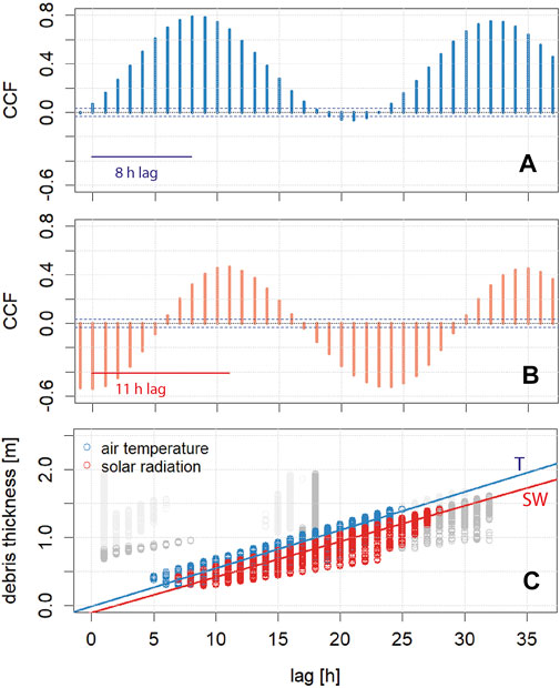
FIGURE 12. (A) Correlogram showing the cross-correlation function (CCF) between air temperature and melt at a pixel with 51 cm debris thickness. (B) CCF between solar radiation and melt at the same pixel. Horizontal blue lines show the 95% confidence interval. (C) Lag derived from the CCF at all pixels against debris thickness. Grey values have no positive correlation and are not considered for the regression.

To derive the remaining parameters, we minimized RMSE and MBE and maximized the NSE (Byrd et al., 1995) against the hourly values computed with the best performing energy balance model, using the median debris conductivity of 1.41 W m⁻¹ K⁻¹. Resulting parameters for the dTI are TF₁ = 0.029 and TF₂ = -0.919 and TF₁ = 0.034, TF₂ = 0.845, SRF₁ = -0.0002 and SRF₂ = −0.31 for the dETI. Additionally, we also tested the same approach for specific thickness classes, yielding different parameters for each subset, which allows for individual application on glaciers depending on their average thickness (Supplementary Table S3).

The dETI model does have a higher NSE (0.68 over 0.58 for the dTI) and reproduces the melt rate better for thinner debris in particular. However the optimized SRF₁ is negative, i.e. additional solar radiation would result in reduced energy for melt. While theoretically possible, it is unlikely to represent a correct reproduction of a physical process. Carenzo et al. (2016) also found that SRF₁ approaches zero towards a debris thickness of 0.5 m. It is likely that in their case it would also turn negative for even thicker debris layers. The TF factors for the dETI model correspond very closely to the values found in Ragettli et al. (2015), while their SRF factors are positive but very small. As both RMSE and MBE are not different for either approach, the only improvement from the solar radiation comes in small shifts in the diurnal cycle.

While the index models are able to accurately simulate the melt peak over different thicknesses, they over- and underestimate the low melt for thin and thick debris, respectively (Figures 13A,B). This can be explained by the fact that both air temperature and incoming solar radiation are not a proxy for the cooling and drying process of debris. This does not have significant effects on cumulative melt neither for thick nor thin debris, however, as that is well simulated with the index models (Figure 13C). Index models poorly reproduce hourly melt for debris thicknesses beyond half a meter as shown here and in previous studies (Ragettli et al., 2015; Carenzo et al., 2016). Unless the interplay between atmospheric forcing and drying and wetting debris is better understood, it is unlikely that parametrizations based on temperature (and other atmospheric variables) will be further improved. On a daily or seasonal scale, the application of a temperature index model with only two free parameters provides satisfying results.

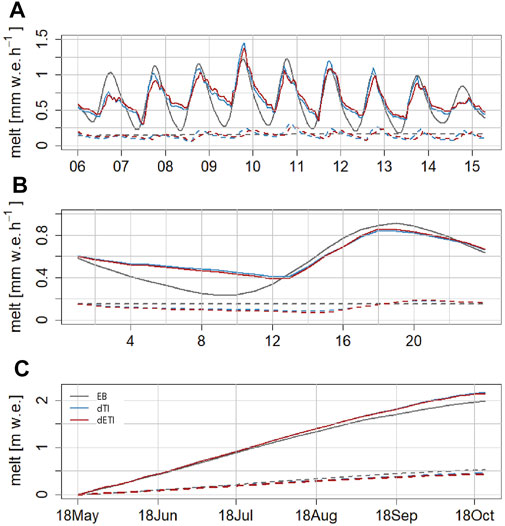
FIGURE 13. Melt curves for two pixels with a debris thickness of 36 (solid) and 181 cm (dashed lines) respectively during nine days in June 2013 (A), the diurnal cycle over the whole season (B) and cumulatively over the whole season (C), calculated with the full energy balance model as well as the two index models.

Validation in Space and Time

The mean mass loss rate based on the dTI model in 2013 over the whole domain (0.82 m ± 0.48 m) reproduced the average observed melt (0.89 m ± 0.76 m) well and the MBE is relatively small (0.07 m). However, the model performance for individual pixels is poor (NSE = −0.2, RMSE = 0.83 m), which is explained by the inaccuracy of the debris thickness as well as our lack of knowledge regarding the variability of conductivity in space.

The dTI model was calibrated with on-glacier data. In catchment scale studies over a longer period of time such datasets are often not available. Therefore we also evaluate the model using off-glacier station data. We already showed that lapsing off-glacier temperature data works reasonably well, with the caveat that warm temperatures over debris during the monsoon are underestimated (Figure 6). We have 4 DEM pairs from Lirung Glacier that are matched by temperature data, namely the monsoon seasons of 2013 and 2016, as well as the winter season 2015 to 2016 and 2017 to 2018 (Supplementary Table S1). With the exception of the last winter season, the median mass loss over the debris-covered surface is matched well by the simple dTI model using off-glacier forcing, with three important caveats; very low, very high melt rates and inter-annual trends (Figure 14). While the median melt rate is well reproduced for both the high (MBE of −0.03 and −0.15 m for 2013 and 2015 respectively) and the low melt season (0.06 and 0.22 for 2015 and 2017), the model has a much smaller spread, especially in the winter season. Very low observed melt rates can be explained by an underestimation of the emergence flux or when ice melt was counterbalanced by redistributed debris, which is obviously not captured separately, as well as by refreezing processes described earlier. The lowest modeled melt rate in winter is 0.5 mm day⁻¹. The very high melt rates (>8 m yr⁻¹, which correspond to a melt rate of >2 cm d⁻¹) are associated to regions around rapidly melting ice cliffs, ice below ponds and the terminus. Accounting for the mass loss on the margins of ice cliffs and along the cliff-pond interface remains challenging (Buri et al., 2016a; Miles et al., 2016) and has so far not been attempted in distributed energy balance models. Any processes related to cliffs or ponds are not captured by a simple index model, but could be incorporated in future by different surface classifications and separate parameters for these surface types.

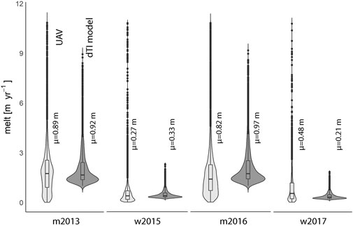
FIGURE 14. Ice melt below debris for two monsoon (m) and two winter seasons (w, see Supplementary Table S1 for exact time periods), measured by DEM differencing (UAV) and modeled with the dTI model.

Finally, it is obvious, that temperature alone does not seem useful to individually explain the differences in mass loss between years. While the observed mass loss decreased between the two monsoon seasons and increased between the winter seasons, the model results do not reproduce this (Figure 14). While temperature alone allows us to get the order of magnitude right and hence provides a valuable input for the catchment scale water balance, more knowledge of the glacier surface, including the debris properties and occurrence of features like cliffs and ponds is necessary to describe the temporal evolution of melt of debris-covered glaciers.

Conclusion

In this study we combine modeling with a unique number of observed datasets from the debris-covered Lirung Glacier, to quantify mass loss in time and space using an energy balance model as well as two index models. The two overarching goals were to evaluate the performance of an energy balance model to reproduce melt at an hourly resolution over a debris-covered tongue, and test the applicability of a computationally fast, but simpler index model to be applied at larger scale.

As a first step we derived a debris thickness map, by inverting the Østrem curve. Comparison to in-situ thickness measurements show this to be a viable approach for the glacier scale, with a MAE of 0.22 m and a MBE of −0.005 m. The results reveal large spatial variability, which ultimately leads to heterogeneous sub-debris melt rates and is likely one of the factors explaining the characteristic hummocky surface morphology of the glacier.

Direct measurements of debris properties show strong variation in texture and associated moisture content with depth. We show that the debris moisture content increases from <0.05 m³ m⁻³ in the upper 10% of the debris to >0.15 m³ m⁻³ above the debris-ice interface (μ = 0.09 m³ m⁻³), even during the drier seasons. As temperature profiles are relatively constant between different locations, we conclude that variability in thermal conductivity of the debris is mainly driven by the varying moisture content. The median thermal conductivity measured in the field (1.29 J m⁻¹ K⁻¹) agrees well with the calibrated conductivity range of our full energy balance model at the location of the AWS (1.1–1.9 J m⁻¹ K⁻¹ for the best matching simulations) as well as for the entire glacier tongue (1.41 J m⁻¹ K⁻¹). We conclude, however, that variability in thermal conductivity remains the single most sensitive variable in our estimates of sub-debris melt. Approaching a debris-covered glacier with lessons from unsaturated zone hydrology as well as permafrost studies could therefore advance our understanding of its mass loss processes. Future investigations should focus on incorporating the spatial (in extent as well as in depth) and temporal heterogeneity of thermal conductivity by considering convective processes and refreezing within the debris pack. For eventual melt water output the retention time of debris as a function of its variable packing density will equally be crucial before including its melt water in catchment wide streamflow.

Using direct hourly surface height change measurements at an AWS on the glacier, we are able to show that the energy balance model reproduces melt rates well over multiple days. Using UAV-derived DEMs, we also conclude that the model reproduces the overall mass loss after an entire melt season for a large part of the glacier tongue well. We also show that using only a single UAV-derived map of seasonal mass balance differences as calibration for the energy balance model produces very similar results as using continuous point-based surface temperature measurements. Moreover, this approach is less prone to temperature measurement uncertainties.

When the conductivity is calibrated in the model, we reproduce the observed mass loss over the complete glacier surface accurately (RMSE of 0.29 cm d⁻¹ and MBE of 0.04 cm d⁻¹) including its spatial patterns. Only very high melt rates that occur at the terminus and in the vicinity of supraglacial cliffs and ponds are not captured. When a constant conductivity for the whole glacier is used, the total mass loss can still be reproduced accurately, but spatial patterns are logically represented less well.

Finally, we test a temperature index model that includes the time lag required for energy to travel through the debris layer, and compare its results against the energy balance model. We show that an index model relying on air temperature (dTI) only performs similar to a model that also includes a solar radiation parameterization (dETI). While these simple models do not accurately capture diurnal melt patterns, they perform satisfactorily in quantifying total melt and we conclude that for catchment scale studies and transient simulations the dTI approach that includes the time lag is most suitable and technically feasible.

Data Availability Statement

Datasets presented in this study can be found in online repositories. Data from AWS Kyanjing can be accessed from https://doi.org/10.26066/RDS.22464, all data collected from UAV flights can be accessed from https://zenodo.org/record/3824264#.YBz0xuA3EWo. Data from AWS and debris on the glacier can be accessed via the authors.

Author Contributions

JS and WI conceptualized the study and collected data. JS executed the analysis and wrote the manuscript with the assistance of WI and PK. PK provided data from UAV flights.

Funding

This project was supported by funding from the European Research Council (ERC) under the European Union’s Horizon 2020 research and innovation program (grant agreement no. 676819) and by the research programme VIDI with project number 016.161.308 financed by Netherlands Organisation for Scientific Research (NWO). The views and interpretations in this publication are those of the authors and they are not necessarily attributable to their organizations.

Conflict of Interest

The authors declare that the research was conducted in the absence of any commercial or financial relationships that could be construed as a potential conflict of interest.

Acknowledgments

We acknowledge the help of numerous people who have participated in field work that made this work possible, including porters and Sirdars from our trekking agency that assisted in the work. We are grateful to Francesca Pellicciotti, Pascal Buri, Evan Miles and all other team members for data collected on Lirung Glacier between 2012 and 2014. We kindly acknowledge Michael McCarthy for providing the GPR data of debris thickness.

Supplementary Material

The Supplementary Material for this article can be found online at: https://www.frontiersin.org/articles/10.3389/feart.2021.678375/full#supplementary-material

References

Anderson, L. S., and Anderson, R. S. (2018). Debris Thickness Patterns on Debris-Covered Glaciers. Geomorphology. 311, 1–12. doi:10.1016/j.geomorph.2018.03.014
Barr, I., Dokukin, M., Kougkoulos, I., Livingstone, S., Lovell, H., Małecki, J., et al. (2018). Using ArcticDEM to Analyse the Dimensions and Dynamics of Debris-Covered Glaciers in Kamchatka, Russia. Geosciences 8 (6), 216. doi:10.3390/geosciences8060216
Basnett, S., Kulkarni, A. V., and Bolch, T. (2013). The Influence of Debris Cover and Glacial Lakes on the Recession of Glaciers in Sikkim Himalaya, India. J. Glaciol. 59 (218), 1035–1046. doi:10.3189/2013JoG12J184
Benn, D. I., Bolch, T., Hands, K., Gulley, J., Luckman, A., Nicholson, L. I., et al. (2012). Response of Debris-Covered Glaciers in the Mount Everest Region to Recent Warming, and Implications for Outburst Flood Hazards. Earth-Science Rev. 114 (1), 156–174. doi:10.1016/j.earscirev.2012.03.008
Bolch, T., Kulkarni, A., Kääb, A., Huggel, C., Paul, F., Cogley, J. G., et al. (2012). The State and Fate of Himalayan Glaciers. Science 336 (6079), 310–314. doi:10.1126/science.1215828
Bonekamp, P. N. J., van Heerwaarden, C. C., Steiner, J. F., and Immerzeel, W. W. (2020). Using 3D Turbulence-Resolving Simulations to Understand the Impact of Surface Properties on the Energy Balance of a Debris-Covered Glacier. The Cryosphere. 14 (5), 1611–1632. doi:10.5194/tc-14-1611-2020
Brock, B. W., Mihalcea, C., Kirkbride, M. P., Diolaiuti, G., Cutler, M. E. J., and Smiraglia, C. (2010). Meteorology and Surface Energy Fluxes in the 2005-2007 Ablation Seasons at the Miage Debris-Covered Glacier, Mont Blanc Massif, Italian Alps. J. Geophys. Res. 115 (D9). doi:10.1029/2009JD013224
Brun, F., Buri, P., Miles, E. S., Wagnon, P., Steiner, J., Berthier, E., et al. (2016). Quantifying Volume Loss from Ice Cliffs on Debris-Covered Glaciers Using High-Resolution Terrestrial and Aerial Photogrammetry. J. Glaciol. 62 (234), 684–695. doi:10.1017/jog.2016.54
Brun, F., Wagnon, P., Berthier, E., Shea, J. M., Immerzeel, W. W., Kraaijenbrink, P. D. A., et al. (2018). Ice Cliff Contribution to the Tongue-wide Ablation of Changri Nup Glacier, Nepal, Central Himalaya. The Cryosphere. 12 (11), 3439–3457. doi:10.5194/tc-12-3439-2018
Buri, P., Miles, E. S., Steiner, J. F., Immerzeel, W. W., Wagnon, P., and Pellicciotti, F. (2016a). A Physically Based 3‐D Model of Ice Cliff Evolution over Debris‐covered Glaciers. J. Geophys. Res. Earth Surf. 121, 2471–2493. doi:10.1002/2016jf004039
Buri, P., Pellicciotti, F., Steiner, J. F., Miles, E. S., and Immerzeel, W. W. (2016b). A Grid-Based Model of Backwasting of Supraglacial Ice Cliffs on Debris-Covered Glaciers. Ann. Glaciol. 57 (71), 199–211. doi:10.3189/2016AoG71A059
Byrd, R. H., Lu, P., Nocedal, J., and Zhu, C. (1995). A Limited Memory Algorithm for Bound Constrained Optimization. SIAM J. Sci. Comput. 16 (5), 1190–1208. doi:10.1137/0916069
Carenzo, M., Pellicciotti, F., Mabillard, J., Reid, T., and Brock, B. W. (2016). An Enhanced Temperature index Model for Debris-Covered Glaciers Accounting for Thickness Effect. Adv. Water Resour. 94, 457–469. doi:10.1016/j.advwatres.2016.05.001
Chand, M. B., Kayastha, R. B., Parajuli, A., and Mool, P. K. (2015). Seasonal Variation of Ice Melting on Varying Layers of Debris of Lirung Glacier, Langtang Valley, Nepal. Proc. IAHS. 368, 21–26. doi:10.5194/piahs-368-21-2015
Collier, E., Nicholson, L. I., Brock, B. W., Maussion, F., Essery, R., and Bush, A. B. G. (2014). Representing Moisture Fluxes and Phase Changes in Glacier Debris Cover Using a Reservoir Approach. The Cryosphere. 8 (4), 1429–1444. doi:10.5194/tc-8-1429-2014
Conway, H., and Rasmussen, L. A. (2000). Summer Temperature Profiles within Supraglacial Debris on Khumbu Glacier, Nepal. IAHS Proc. n. 264, 89–97.
Cuffey, K. M., and Paterson, W. S. B. (2010). The Physics of Glaciers. 4th Edition. Academic PressAvailable at: https://www.elsevier.com/books/the-physics-of-glaciers/cuffey/978-0-12-369461-4.
Dehecq, A. N., Gourmelen, A. S., Gardner, F., Brun, D., Goldberg, P. W., Nienow, E., et al. (2019). Twenty-First Century Glacier Slowdown Driven by Mass Loss in High Mountain Asia. Nat. Geosci. 12 (1), 22–27. doi:10.1038/s41561-018-0271-9
Farinotti, D., Huss, M., Fürst, J. J., Landmann, J., Machguth, H., Maussion, F., et al. (2019). A Consensus Estimate for the Ice Thickness Distribution of All Glaciers on Earth. Nat. Geosci. 12 (3), 168–173. doi:10.1038/s41561-019-0300-3
Foster, L. A., Brock, B. W., Cutler, M. E. J., and Diotri, F. (2012). A Physically Based Method for Estimating Supraglacial Debris Thickness from Thermal Band Remote-Sensing Data. J. Glaciol. 58 (210), 677–691. doi:10.3189/2012JoG11J194
Fujita, K., and Sakai, A. (2000). Air Temperature Environment on the Debris- Covered Area of Lirung Glacier, Langtang Valley, Nepal Himalayas. IAHS Proc. n. 264, 83–88.
Fyffe, C. L., Reid, T. D., Brock, B. W., Kirkbride, M. P., Diolaiuti, G., Smiraglia, C., et al. (2014). A Distributed Energy-Balance Melt Model of an Alpine Debris-Covered Glacier. J. Glaciol. 60 (221), 587–602. doi:10.3189/2014JoG13J148
Fyffe, C. L., Woodget, A. S., Kirkbride, M. P., Deline, P., Westoby, M. J., and Brock, B. W. (2020). Processes at the Margins of Supraglacial Debris Cover: Quantifying Dirty Ice Ablation and Debris Redistribution. Earth Surf. Process. Landforms. 45, 2272–2290. doi:10.1002/esp.4879
Gardelle, J., Berthier, E., and Arnaud, Y. (2012). Slight Mass Gain of Karakoram Glaciers in the Early Twenty-First Century. Nat. Geosci. 5 (5), 322–325. doi:10.1038/ngeo1450
Genuchten, M. Th. van. (1980). A Closed-form Equation for Predicting the Hydraulic Conductivity of Unsaturated Soils. Soil Sci. Soc. America J. 44 (5), 892–898. doi:10.2136/sssaj1980.03615995004400050002x
Giese, A., Boone, A., Wagnon, P., and Hawley, R. (2020). Incorporating Moisture Content in Surface Energy Balance Modeling of a Debris-Covered Glacier. The Cryosphere 14 (5), 1555–1577. doi:10.5194/tc-14-1555-2020
Herreid, S., and Pellicciotti, F. (2018). Automated Detection of Ice Cliffs within Supraglacial Debris Cover. The Cryosphere 12 (5), 1811–1829. doi:10.5194/tc-12-1811-2018
Heynen, M., Miles, E., Ragettli, S., Buri, P., Immerzeel, W. W., and Pellicciotti, F. (2016). Air Temperature Variability in a High-Elevation Himalayan Catchment. Ann. Glaciol. 57 (71), 212–222. doi:10.3189/2016AoG71A076
Hock, R. (1999). A Distributed Temperature-Index Ice- and Snowmelt Model Including Potential Direct Solar Radiation. J. Glaciol. 45 (149), 101–111. doi:10.3189/S0022143000003087
Immerzeel, W. W., Kraaijenbrink, P. D. A., Shea, J. M., Shrestha, A. B., Pellicciotti, F., Bierkens, M. F. P., et al. (2014a). High-Resolution Monitoring of Himalayan Glacier Dynamics Using Unmanned Aerial Vehicles. Remote Sensing Environ. 150, 93–103. doi:10.1016/j.rse.2014.04.025
Immerzeel, W. W., Petersen, L., Ragettli, S., and Pellicciotti, F. (2014b). The Importance of Observed Gradients of Air Temperature and Precipitation for Modeling Runoff from a Glacierized Watershed in the Nepalese Himalayas. Water Resour. Res. 50 (3), 2212–2226. doi:10.1002/2013WR014506
Janke, J. R., Bellisario, A. C., and Ferrando, F. A. (2015). Classification of Debris-Covered Glaciers and Rock Glaciers in the Andes of Central Chile. Geomorphology. 241, 98–121. doi:10.1016/j.geomorph.2015.03.034
Juen, M., Mayer, C., Lambrecht, A., Wirbel, A., and Kueppers, U. (2013). Thermal Properties of a Supraglacial Debris Layer with Respect to Lithology and Grain Size. Geografiska Annaler: Ser. A, Phys. Geogr. 95 (3), 197–209. doi:10.1111/geoa.12011
Kääb, A., Berthier, E., Nuth, C., Gardelle, J., and Arnaud, Y. (2012). Contrasting Patterns of Early Twenty-First-Century Glacier Mass Change in the Himalayas. Nature. 488 (7412), 495–498. doi:10.1038/nature11324
Kayastha, R. B., Takeuchi, Y., Nakawo, M., and Ageta, Y. (2000). Practical Prediction of Ice Melting beneath Various Thickness of Debris Cover on Khumbu Glacier, Nepal, Using a Positive Degree-Day Factor. IAHS Proc. n. 264, 71–81.
Khan, M. I. (1989). Ablation on Barpu Glacier, Karakoram Himalaya, Pakistan a Study of Melt Processes on a Faceted, Debris-Covered Ice Surface. MSc Thesis. Waterloo: Wilfrid Laurier University.
Kok, R. J., Steiner, J. F., Litt, M., Wagnon, P., Koch, I., Wagnon, P., et al. (2019). Measurements, Models and Drivers of Incoming Longwave Radiation in the Himalaya. Int. J. Climatol. 40 (2), 942–956. doi:10.1002/joc.6249
Kraaijenbrink, P. D. A., Bierkens, M. F. P., Lutz, A. F., and Immerzeel, W. W. (2017). Impact of a Global Temperature Rise of 1.5 Degrees Celsius on Asia's Glaciers. Nature. 549 (7671), 257–260. doi:10.1038/nature23878
Kraaijenbrink, P. D. A., and Immerzeel, W. W. (2020). Unmanned Aerial Vehicle Data of Lirung Glacier and Langtang Glacier for 2013–2018 (Version 1.0.0) [Data set]. Zenodo. doi:10.5281/zenodo.3824264
Kraaijenbrink, P. D. A., Shea, J. M., Litt, M., Steiner, J. F., Treichler, D., Koch, I., et al. (2018). Mapping Surface Temperatures on a Debris-Covered Glacier with an Unmanned Aerial Vehicle. Front. Earth Sci. 6, 1. doi:10.3389/feart.2018.00064
Kraaijenbrink, P. D. A., Meijer, S. W., Shea, J. M., Pellicciotti, F., De Jong, S. M., and Immerzeel, W. W. (2016a). Seasonal Surface Velocities of a Himalayan Glacier Derived by Automated Correlation of Unmanned Aerial Vehicle Imagery. Ann. Glaciol. 57 (71), 103–113. doi:10.3189/2016AoG71A072
Kraaijenbrink, P. D. A., Shea, J. M., Pellicciotti, F., Jong, S. M. d., and Immerzeel, W. W. (2016b). Object-Based Analysis of Unmanned Aerial Vehicle Imagery to Map and Characterise Surface Features on a Debris-Covered Glacier. Remote Sensing Environ. 186, 581–595. doi:10.1016/j.rse.2016.09.013
Lambrecht, A., Mayer, C., Hagg, W., Popovnin, V., Rezepkin, A., Lomidze, N., et al. (2011). A Comparison of Glacier Melt on Debris-Covered Glaciers in the Northern and Southern Caucasus. The Cryosphere. 5 (3), 525–538. doi:10.5194/tc-5-525-2011
Loomis, S. R. (1970). Morphology and Ablation Processes on Glacier Ice. Assoc. Am. Geogr. Proc. 2, 88–92.
Macfarlane, A. M., Hodges, K. V., and Lux, D. (1992). A Structural Analysis of the Main Central Thrust Zone, Langtang National Park, Central Nepal Himalaya. GSA Bull. 104 (11), 1389–1402. doi:10.1130/0016-7606(1992)104<1389:asaotm>2.3.co;2
McCarthy, M., Pritchard, H., Willis, I., and King, E. (2017). Ground-Penetrating Radar Measurements of Debris Thickness on Lirung Glacier, Nepal. J. Glaciol. 63 (239), 543–555. doi:10.1017/jog.2017.18
Midgley, N. G., Tonkin, T. N., Graham, D. J., and Cook, S. J. (2018). Evolution of High-Arctic Glacial Landforms during Deglaciation. Geomorphology. 311, 63–75. doi:10.1016/j.geomorph.2018.03.027
Miles, E. S., Pellicciotti, F., Willis, I. C., Steiner, J. F., Buri, P., and Arnold, N. S. (2016). Refined Energy-Balance Modeling of a Supraglacial Pond, Langtang Khola, Nepal. Ann. Glaciol. 57 (71), 29–40. doi:10.3189/2016AoG71A421
Miles, E. S., Steiner, J. F., and Brun, F. (2017a). Highly Variable Aerodynamic Roughness Length (Z 0 ) for a Hummocky Debris-Covered Glacier. J. Geophys. Res. Atmos. 122 (16), 8447–8466. doi:10.1002/2017JD026510
Miles, E. S., Steiner, J., Willis, I., Buri, P., Immerzeel, W. W., Chesnokova, A., et al. (2017b). Pond Dynamics and Supraglacial-Englacial Connectivity on Debris-Covered Lirung Glacier, Nepal. Front. Earth Sci. 5, 69. doi:10.3389/feart.2017.00069
Naylor, M. A. (1980). The Origin of Inverse Grading in Muddy Debris Flow Deposits; a Review. J. Sediment. Res. 50 (4), 1111–1116. doi:10.1306/212F7B8F-2B24-11D7-8648000102C1865D
Nicholson, L., and Benn, D. I. (2006). Calculating Ice Melt beneath a Debris Layer Using Meteorological Data. J. Glaciol. 52 (178), 463–470. doi:10.3189/172756506781828584
Nicholson, L., and Benn, D. I. (2013). Properties of Natural Supraglacial Debris in Relation to Modeling Sub-debris Ice Ablation. Earth Surf. Process. Landforms. 38 (5), 490–501. doi:10.1002/esp.3299
Nicholson, L. I., McCarthy, M., Pritchard, H. D., and Willis, I. (2018). Supraglacial Debris Thickness Variability: Impact on Ablation and Relation to Terrain Properties. The Cryosphere. 12 (12), 3719–3734. doi:10.5194/tc-12-3719-2018
Nuimura, T., Fujita, K., Yamaguchi, S., and Sharma, R. R. (2012). Elevation Changes of Glaciers Revealed by Multitemporal Digital Elevation Models Calibrated by GPS Survey in the Khumbu Region, Nepal Himalaya, 1992-2008. J. Glaciol. 58 (210), 648–656. doi:10.3189/2012JoG11J061
Östrem, G. (1959). Ice Melting under a Thin Layer of Moraine, and the Existence of Ice Cores in Moraine Ridges. Geografiska Annaler. 41 (4), 228–230. doi:10.1080/20014422.1959.11907953
Pellicciotti, F., Brock, B., Strasser, U., Burlando, P., Funk, M., and Corripio, J. (2005). An Enhanced Temperature-index Glacier Melt Model Including the Shortwave Radiation Balance: Development and Testing for Haut Glacier d'Arolla, Switzerland. J. Glaciol. 51 (175), 573–587. doi:10.3189/172756505781829124
Popovnin, V. V., and Rozova, A. V. (2002). Influence of Sub-debris Thawing on Ablation and Runoff of the Djankuat Glacier in the Caucasus. Nordic Hydrol. 33 (I), 75–94. doi:10.2166/nh.2002.0005
Ragettli, S., Bolch, T., and Pellicciotti, F. (2016). Heterogeneous Glacier Thinning Patterns over the Last 40 Years in Langtang Himal, Nepal. The Cryosphere 10 (5), 2075–2097. doi:10.5194/tc-10-2075-2016
Ragettli, S., Pellicciotti, F., Immerzeel, W. W., Miles, E. S., Petersen, L., Heynen, M., et al. (2015). Unraveling the Hydrology of a Himalayan Catchment through Integration of High Resolution In Situ Data and Remote Sensing with an Advanced Simulation Model. Adv. Water Resour. 78, 94–111. doi:10.1016/j.advwatres.2015.01.013
Reid, T. D., and Brock, B. W. (2010). An Energy-Balance Model for Debris-Covered Glaciers Including Heat Conduction through the Debris Layer. J. Glaciol. 56 (199), 903–916. doi:10.3189/002214310794457218
Reid, T. D., Carenzo, M., Pellicciotti, F., and Brock, B. W. (2012). Including Debris Cover Effects in a Distributed Model of Glacier Ablation. J. Geophys. Res. 117 (D18), a–n. doi:10.1029/2012JD017795
Rounce, D. R., King, O., McCarthy, M., Shean, D. E., and Salerno, F. (2018). Quantifying Debris Thickness of Debris‐Covered Glaciers in the Everest Region of Nepal through Inversion of a Subdebris Melt Model. J. Geophys. Res. Earth Surf. 123 (5), 1094–1115. doi:10.1029/2017JF004395
Rounce, D. R., and McKinney, D. C. (2014). Debris Thickness of Glaciers in the Everest Area (Nepal Himalaya) Derived from Satellite Imagery Using a Nonlinear Energy Balance Model. The Cryosphere. 8 (4), 1317–1329. doi:10.5194/tc-8-1317-2014
Rounce, D. R., Quincey, D. J., and McKinney, D. C. (2015). Debris-covered Glacier Energy Balance Model for Imja-Lhotse Shar Glacier in the Everest Region of Nepal. The Cryosphere. 9 (6), 2295–2310. doi:10.5194/tc-9-2295-2015
Rowan, A. V., Nicholson, L. I., Quincey, D. J., Gibson, M. J., Irvine-Fynn, T. D. L., Watson, C. S., et al. (2020). Seasonally Stable Temperature Gradients through Supraglacial Debris in the Everest Region of Nepal, Central Himalaya. J. Glaciol. 67, 170. doi:10.1017/jog.2020.100
Sakai, A., Nakawo, M., and Fujita, K. (2002). Distribution Characteristics and Energy Balance of Ice Cliffs on Debris-Covered Glaciers, Nepal Himalaya. Arctic, Antarctic, Alpine Res. 34 (1), 12–19. doi:10.2307/155250310.1080/15230430.2002.12003463
Sakai, A., Takeuchi, N., Fujita, K., and Nakawo, M. (2000). Role of Supraglacial Ponds in the Ablation Process of a Debris-Covered Glacier in the Nepal Himalayas. IAHS Proc. 265, 119–130.
Schauwecker, S., Rohrer, M., Huggel, C., Kulkarni, A., Ramanathan, A., Salzmann, N., et al. (2015). Remotely Sensed Debris Thickness Mapping of Bara Shigri Glacier, Indian Himalaya. J. Glaciol. 61 (228), 675–688. doi:10.3189/2015JoG14J102
Scherler, D., Bookhagen, B., and Strecker, M. R. (2011). Hillslope-Glacier Coupling: The Interplay of Topography and Glacial Dynamics in High Asia. J. Geophys. Res. 116 (March), 1–21. doi:10.1029/2010JF001751
Shaw, T. E., Brock, B. W., Fyffe, C. L., Pellicciotti, F., Rutter, N., and Diotri, F. (2016). Air Temperature Distribution and Energy-Balance Modeling of a Debris-Covered Glacier. J. Glaciol. 62 (231), 185–198. doi:10.1017/jog.2016.31
Steiner, J. F., Buri, P., Miles, E. S., Ragettli, S., and Pellicciotti, F. (2019). Supraglacial Ice Cliffs and Ponds on Debris-Covered Glaciers: Spatio-Temporal Distribution and Characteristics. J. Glaciol. 65 (252), 617–632. doi:10.1017/jog.2019.40
Steiner, J. F., Litt, M., Stigter, E. E., Shea, J., Bierkens, M. F. P., and Immerzeel, W. W. (2018). The Importance of Turbulent Fluxes in the Surface Energy Balance of a Debris-Covered Glacier in the Himalayas. Front. Earth Sci. 6, 144. doi:10.3389/feart.2018.00144
Steiner, J. F., Pellicciotti, F., Buri, P., Miles, E. S., Immerzeel, W. W., and Reid, T. D. (2015). Modeling Ice-Cliff Backwasting on a Debris-Covered Glacier in the Nepalese Himalaya. J. Glaciol. 61 (229), 889–907. doi:10.3189/2015JoG14J194
Steiner, J. F., and Pellicciotti, F. (2016). Variability of Air Temperature over a Debris-Covered Glacier in the Nepalese Himalaya. Ann. Glaciol. 57 (71), 295–307. doi:10.3189/2016AoG71A066
Watson, C. S., Quincey, D. J., Carrivick, J. L., and Smith, M. W. (2016). The Dynamics of Supraglacial Ponds in the Everest Region, Central Himalaya. Glob. Planet. Change. 142, 14–27. doi:10.1016/j.gloplacha.2016.04.008
Wigmore, O., and Mark, B. (2017). Monitoring Tropical Debris-Covered Glacier Dynamics from High-Resolution Unmanned Aerial Vehicle Photogrammetry, Cordillera Blanca, Peru. The Cryosphere. 11 (6), 2463–2480. doi:10.5194/tc-11-2463-2017
Keywords: debris cover, glacier melt, Himalaya, energy balance, temperature index
Citation: Steiner JF, Kraaijenbrink PDA and Immerzeel WW (2021) Distributed Melt on a Debris-Covered Glacier: Field Observations and Melt Modeling on the Lirung Glacier in the Himalaya. Front. Earth Sci. 9:678375. doi: 10.3389/feart.2021.678375
Received: 09 March 2021; Accepted: 25 June 2021;
Published: 13 July 2021.
Edited by:
Lindsey Isobel Nicholson, University of Innsbruck, AustriaCopyright © 2021 Steiner, Kraaijenbrink and Immerzeel. This is an open-access article distributed under the terms of the Creative Commons Attribution License (CC BY). The use, distribution or reproduction in other forums is permitted, provided the original author(s) and the copyright owner(s) are credited and that the original publication in this journal is cited, in accordance with accepted academic practice. No use, distribution or reproduction is permitted which does not comply with these terms.
*Correspondence: Jakob F. Steiner, jakob.steiner@icimod.org