Low-Frequency Elastic Properties of a Polymineralic Carbonate: Laboratory Measurement and Digital Rock Physics

Introduction

Digital Rock Physics (DRP) applied to carbonates is an important and quickly evolving research topic (e.g., Amabeoku et al., 2013; Saenger et al., 2016; AlJallad et al., 2020; Han et al., 2020), especially regarding the prediction of elastic moduli of polymineralic carbonate rocks. In general, the most common methods in DRP are based on segmentation, which tend to strongly overpredict the elastic moduli of such rocks. It has been suggested that such inaccuracy is due to the inability of segmentation in resolving micro-features, such as pores, grain contacts, and cracks (e.g., Madonna et al., 2012; Andrä et al., 2013a). Carbonate rocks can contain a significant amount of micropores that cannot be resolved by CT imaging (Saenger et al., 2016). In carbonates, pores can lie between mineral grains or particles (interparticle and intercrystal pores), within particles (intraparticle pores), or within mineral grains due to, for instance, dissolution processes (moldic pores). Pores can be smaller than 1 μm (Scholle and Ulmer-Scholle, 2003), which is below the spatial resolution of a typical CT-scanner (Iassonov et al., 2009). One could scan samples at nanometric resolutions, capturing only millimetric volumes that, however, might not be a Representative Elementary Volume (REV) for the studied lithology (Saenger et al., 2016).

Several methods have been proposed to extract sub-resolution features - especially microporosity - from CT-images with a resolution around 10 microns. Sok et al. (2010) introduced the multiscale analysis technique where images of a sample at different resolutions were combined. They scanned a carbonate rock sample at ∼1 micron resolution and recognized three phases in the CT-images: solid grains, resolvable pore spaces, and micropores. The porosity calculated from resolvable pore spaces yielded 11% porosity, whereas the porosity of the sample, measured with the Mercury Injection Capillary Pressure (MICP) technique, was 36%. Therefore, they assumed that approximately 25% of the total pore volume was in micropores. A multiscale analysis estimated the microporosity by stochastically mapping micropores with Scanning Electron Microscopy (SEM). Micro-CT and SEM images were taken at the same locations and registered: the average porosities of the SEM image were paired with the average X-ray attenuation of CT-images. Pairs of average porosities and average X-ray attenuation were used to create an X-ray attenuation-to-porosity calibration curve. Such a multiscale analysis technique estimated a sample porosity of 35%, which agreed with the MICP result. Lin et al. (2016) tackled the sub-resolution porosity problem in the acquisition process. They performed a differential measurement of X-ray attenuation by comparing CT-images of dry and brine saturated samples. Lin et al. (2016) concluded that the sub-resolution porosity contributed to up to 10% of the total porosity of the sample. Other authors have proposed methods to incorporate sub-resolution information from CT data. Such approaches rely on the local variation of X-ray attenuation to estimate effective rock properties such as density and porosity (e.g., Taud et al., 2005; Dunsmuir et al., 2006; Gupta et al., 2018).

To estimate the effect of sub-resolution features on elastic properties, several methods have been proposed. Tisato and Spikes (2016) introduced a DRP technique that does not require segmentation. Their method relies on homogenization theory, where the spatial distribution of elastic properties is the interpolation between the elastic properties of the materials composing the rock. The interpolation function depends on the chosen effective medium theory (EMT). As a result, each voxel is assigned a specific elastic modulus that depends on the X-ray attenuation. The method was tested on a Berea Sandstone, yielding results that agreed with laboratory measurements. Ikeda et al. (2020) furthered the study of Tisato and Spikes (2016) by introducing the Segmentation-Less method withOut Targets (SLOT) that do not require calibration targets - often referred to as phantoms in the CT community.

Saenger et al. (2016) proposed a method called “two-phase wave propagation simulations” to obtain porosity dependent P and S-wave velocities of sedimentary rocks. They created several CT derived digital rock models by varying the segmentation threshold of the CT number used to separate the solid phase (calcite) from the pore phase (vacuum). As a consequence, each model had a different porosity. Each model underwent numerical simulations where the results were used to obtain effective P-wave and S-wave velocities. The variation of P and S-wave velocities with porosity were used to create velocity bounds for the lithology. Sun et al. (2017) performed a multiscale analysis on carbonate CT-images to predict elastic properties. Some estimated physical properties agreed with the laboratory measurements except for the P-wave and the S-wave velocities. Nonetheless, both methods approaches have not been used on carbonate samples containing both dolomite and calcite.

Here, we propose a modified segmentation-less method (modified-SLOT), which is based on the SLOT algorithm whose main limitation is that it can be applied only on monomineralic rocks. The present work relaxes such a limitation, allowing the estimation of elastic properties of polymineralic rocks from CT-images. Numerical simulation results are compared to low-frequency sub-resonance laboratory measurements and segmentation-based DRP. The proposed methodology, modified-SLOT, estimates static Young’s modulus of a polymineralic carbonate sample within 10% of laboratory measurements.

Materials and Methods

Description of the Physical Sample

Our sample was collected from the pre-salt Barra Velha formation of the Santos Basin in Brazil (Gomes et al., 2020). The formation contains massive to cross stratified units. The sample is a lacustrine carbonate formed in the early stages of the Atlantic ocean rifting and was cored from a facies of reworked carbonate shrubs and spherulites. Spherulites are spherical to sub-spherical allochems, that in the Barra Velha formation are commonly dolomitized with secondary porosity. Shrubs are aggregated fibrous to coarse bladed calcite crystals (Wright & Barnett, 2015; Chafetz et al., 2018).

The original sample was a cylinder of size 25.4 cm in diameter and ∼100 mm in length. A cylindrical plug of size 25.4 mm in diameter and 62.4 mm in length was obtained from the original sample. Such a sample is called sample A, and it was used for the measurement of Young’s modulus and attenuation at frequencies in the range 1–100 Hz (Figure 1A). The porosity of the sample A is ϕ_lab = 15.5%. The remaining sample was cored to obtain a small cylinder of size 8 mm in diameter and few mm in length - sample B (Figure 1B). We used X-ray micro-computed tomography (micro-CT) to obtain a 3D digital model of one of the 8 mm core plugs (Figures 1C,D). The remainder of the original sample comprised three samples with no regular shape that were used for mercury injection capillary pressure tests (MICP), namely sample C, sample D, and sample E (Figure 1E).

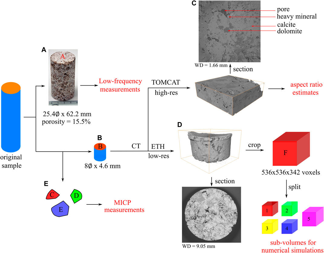
FIGURE 1. Sample descriptions and workflow of the process. The original sample was cut into sample (A) for the low-frequency measurement. The remaining part of the sample was used for CT-scan (sample B) and MICP measurement (sample C–E). Sample (B) was scanned at two facilities: TOMCAT and ETH. The TOMCAT scan provided high-resolution images in which we use for estimating aspect ratio of pore spaces. The ETH scan, whose resolution was lower, covered more area of the sample and was used for numerical simulations. The ruler in the sample (A) figure is in centimeters and WD represents the width of the image.

MICP analyses were performed at the claylab of the Swiss Federal Institute of Technology Zurich (ETH Zürich, Switzerland) by means of a Pascal 140 + 440 instrument from POROTEC (Hofheim am Taunus, Germany). The MICP porosities for samples C, D, and E are 14.99%, 17.65%, and 14.39%, respectively; and the average of such measurements is 15.7%, which is 0.2% higher than ϕ_lab. Figure 1 provides a synoptic panel reporting the samples and the tests performed. The MICP test (Figure 2) also indicates that some pores have a radius below 50 µm (∼6%). Most of the pore throats lie in the range 10³–10⁴ μm (Figure 2). Note that MICP only measures the connected porosity of the sample.

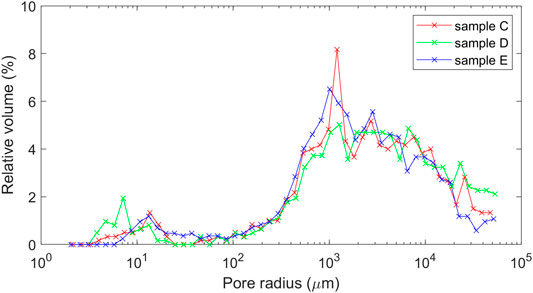
FIGURE 2. MICP data for the carbonate sample investigated. Here, we show the result obtained from one of the core plugs.

Description of the CT-Dataset

We collected 3D images of sample B by means of X-ray micro-computed tomography (ETH dataset) and synchrotron X-ray tomography (TOMCAT dataset). The ETH dataset was obtained at the Swiss Federal Institute of Technology Zurich (ETH Zürich, Switzerland) using a phoenix v|tome|x 240 X-ray scanner (GE Sensing & Inspection Technologies GmbH, Germany). The X-ray tube voltage and current were 150 kV and 65 μA, respectively. We used a 0.5 mm copper filter to minimize beam hardening. Images were taken every 0.2° for an entire revolution. The final reconstructed 3D volume had a voxel size of 9.88 microns and a cross-section of 916 × 869 pixels. The spatial distribution of X-ray attenuation was scaled and stored as an array of 16-bit integers, known as CT-numbers (Ketcham and Carlson, 2001). CT-number is a proxy for the density of the material irradiated by the X-rays (Mull, 1984). Figures 1C,D show an arbitrary cross-section from the micro-CT data. The resolution of our scan was not high enough to resolve all the features within the sample, such as small pores and microcracks. Only the bigger pores were resolved, appearing as a dark color in the micro-CT images. The ETH dataset was then used to compute the elastic properties of the sample. In particular, we extracted a sub-volume of size 536 × 536 × 342 voxels from such a dataset (sample F). This volume was the largest artifact-free rectangular volume that could be extracted from the dataset. The CT-images of the sub-volume were processed and visualized with Fiji (Schindelin et al., 2012). We applied a local mean filter with the smoothing factor of 3 and the automatic standard deviation to denoize the CT-images. Then, we applied the statistical region merging to group similar voxels (Buades et al., 2005, p.; Nock and Nielsen, 2004). Due to the limitation of computational resources, we performed the numerical simulations of five cascaded sub-volumes extracted from sample F (Figures 1, 3). The location of each sub-volume is listed in Table 1. The first four sub-volumes are 300 × 300 × 300 voxels in size. The fifth sub-volume, on the other hand, is 350 × 350 × 300 voxels in size. The fifth sub-volume was intentionally chosen, such that its porosity was 15.44% i.e., only 0.06% from ${\varnothing }_{\text{lab}}$.

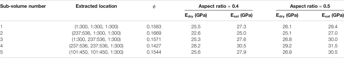
TABLE 1. Numerical simulation results from the modified-SLOT.

On the other hand, the synchrotron TOMCAT dataset was obtained at the X-ray Tomographic Microscopy and Coherent rAdiology experimenTs beamline of the Swiss Light Source (SLS; Paul Scherrer Institute, Villigen, Switzerland). The beam energy was 26 keV with 500 ms exposure time. The final reconstructed 3D volume yielded a volume with a section of 2560 × 2560 pixels with a voxel size of 0.65 microns/voxel. Such a scan covers 0.1% of sample B, and its elastic properties might not represent the elastic properties of the lithology under study. However, we assume that the microporosity of the TOMCAT dataset properly represents the microporosity of sample B. Thus, we use such a dataset to estimate the aspect ratio of the micropores.

According to the CT-images, four distinct shades of gray (i.e., CT-numbers clusters) are observed in the CT-images: 1) black, 2) light-gray, 3) dark-gray, and 4) white (Figure 3). Such shades are interpreted to represent 1) air, 2) dolomite, 3) calcite, and 4) a heavy mineral, based on the X-ray attenuation characterization of each material and the petrophysical analyses on the core sample. At our scanning conditions, dolomite attenuates X-rays less than calcite and therefore bears a darker shade (i.e., lower CT-numbers) than calcite (see Supplementary Information) (Chantler et al., 2005; Wang et al., 2013). A first-order analysis of the CT-images shows that the volumetric fractions of voxels classified as air $\left(f_{\text{air}}^{\text{seg}}\right)$, calcite $\left(f_{\text{cal}}^{\text{seg}}\right)$, dolomite $\left(f_{\text{dol}}^{\text{seg}}\right)$, and heavy minerals $\left(f_{\text{heavy}}^{\text{seg}}\right)$ are 8.65%, 69.17%, 22.13%, and 0.05%, respectively.

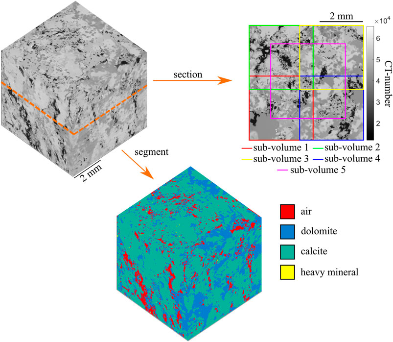
FIGURE 3. A CT-volume of the sample with the interpreted mineral compositions. The CT-volume has been segmented into four phases: air, dolomite, calcite, and heavy mineral. The section of the CT-volume shows the location where sub-volumes have been extracted for the numerical simulations.

As $f_{\text{air}}^{\text{seg}}$ is 8.65% and ${\varphi }_{\text{lab}}$ is 15.5%, we concluded that our sample comprises 6.85% of sub-resolution porosity. Such a mismatch suggests that 6.85% of the porosity cannot be resolved with the ETH dataset. Thus, $f_{\text{cal}}^{\text{seg}}$, $f_{\text{dol}}^{\text{seg}}$, and $f_{\text{heavy}}^{\text{seg}}$, indeed, represent the volume fractions of the minerals plus the sub-resolution porosity, while the actual volume fractions of the minerals are denoted as $V_{\text{cal}}$, $V_{\text{dol}}$, and $V_{\text{heavy}}$ for calcite, dolomite, and heavy mineral, respectively. We neglected the sub-resolution pore spaces in the heavy mineral fraction (i.e., $f_{\text{heavy}}^{\text{seg}}=V_{\text{heavy}}$), because such a phase represents a very tiny portion of the total volume, and minerals such as sulfides and oxides are likely to have limited porosity (<1%) (Baumgartner et al., 2019).

Methods

Laboratory Measurements of Low-Frequency Young’s Modulus

To measure Young’s modulus and attenuation of seismic waves for sample A, we used the Seismic Wave Attenuation Module (SWAM, Madonna and Tisato, 2013). The SWAM uses the forced oscillation method to measure such properties. The measurements were performed at seismic frequencies (1–100 Hz). Table 2 lists the physical properties of the carbonate sample and the aluminum standard that were used as a reference in the laboratory measurements. The SWAM has a piezo actuator to produce a sinusoidal vertical stress, while a couple of Linear Variable Differential Transformers (LVDTs) measures the bulk shortenings of the rock sample and the aluminum standard. Shortenings are recorded by an oscilloscope after amplification (Figure 4). As aluminum is nearly elastic, its shortening can be considered to be in phase with the applied stress. The amplitude ratio and the phase shift between the shortening across the rock sample and across the aluminum standard allowed calculating the sample Young’s modulus and attenuation, respectively.

TABLE 2. Properties of the carbonate sample and aluminum standard.

FIGURE 4. Displacement signals of the sample and aluminum standard at 100 Hz.

The SWAM was placed in a Paterson pressure rig (Paterson and Olgaard, 2000), which employed argon gas as a confining medium. To avoid flow of pore fluid across the curved side of the sample, and to prevent argon from seeping into the sample, a 0.1 mm thick copper jacket was used as a sealing (Figure 5A). The aluminum standard was enclosed in a 0.75 mm thick heat-shrinkable fluorinated ethylene propylene (FEP) tube (Figure 5B). The SWAM was connected to a syringe pump using pipes of 1 mm internal diameter to saturate the sample. Over time, there was a tiny leak of argon into the sample (0.01–0.05 MPa/h, as per the pump reading). The pore pressure system was kept open to the atmosphere so that the gas could escape through the pore fluid pipes. Therefore, during measurements, pore pressure was equal to atmospheric pressure (Subramaniyan et al., 2015).

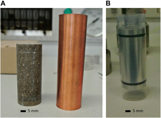
FIGURE 5. Jacketing (A) Copper jacket, used for the carbonate (B) Shrink tube, used for the aluminum standard.

Laboratory measurements were conducted at 5 MPa confining pressure, 20°C temperature, and two fluid saturation conditions: dry and 100% water-saturated. The sample was oven-dried before performing the measurements in dry conditions. Once such a measurement was completed, a water volume corresponding to the desired saturation level (100%) was introduced into the sample. To ensure full saturation, the sample was flushed with a volume of water more than ten times the sample pore volume. While flushing the pressure gradient across the sample was kept at ∼2 MPa. After each saturation step, the pore fluid valves were left open, thereby the pore pressure equilibrated to the atmospheric pressure.

Each series of measurements resulted in 20 data points across the frequency range of 1–100 Hz. By looping five times over the frequency range, we obtained five repetitions of the measurement and the corresponding precision error. Such an error and those corresponding to sample length and LVDTs calibration were propagated into the results of Young’s modulus. The strain across the sample was 2 × 10^–6, hence similar to the strain caused by seismic waves measured in exploration geophysics (Mavko et al., 2020).

Digital Rock Physics on CT-Images

In our study, we simulated the static compression of the digital sample to calculate the effective elastic properties of the sample. The numerical solver employed in this study was elas3D (Garboczi, 1998). Details about the numerical solver will be explained in the next section. Elas3D numerically solves the elastic deformation of the digital sample using the Finite Element method on a cubic mesh. The first step of DRP is to estimate the bulk and shear modulus for each voxel as input parameters for the solver. We considered two methods to define the elastic tensor at each element: a segmentation-based method and a newly developed segmentation-less method. Elements were defined at each voxel in the CT-images, and we assumed that our sample was isotropic.

Segmentation-Less DRP

In our segmentation-less method we consider a voxel being a mixture of two different materials e.g., a mineral (e.g., calcite or dolomite) and air; and we assume that the elastic tensor of the voxel is a weighted average of the elastic properties of the two materials. Two segmentation-less procedures are briefly summarized as follows, and a complete description of such methods can be found in Ikeda et al. (2020).

The Segmentation-Less wIth Targets (SLIT) uses the densities and CT-numbers of reference materials–targets–to calibrate the CT dataset and obtain a density map of the CT imagery. On the other hand, if targets are not scanned along with the sample, the Segmentation-Less withOut Targets (SLOT) could be used. SLOT assumes that extreme CT-numbers within the CT-dataset represent pristine materials to create a CT-number-to-density calibration. The algorithm iteratively optimizes the calibration curve to minimize the difference between ϕ_lab and ϕ_CT, which is the porosity of the CT-imagery dataset - this step is called optimization process. The calibration creates a density model that is then converted to a porosity model. Both the methods use a negative-linear-proportional relationship. For example, to convert the density model to the porosity model, we apply:

where $\varphi \left(\mathbf{X}\right)$ is the porosity at loation $\mathbf{X}$ in the CT-imagery, $\rho \left(\mathbf{X}\right)$ is the density at location $\mathbf{X}$, and ${\rho }_{\text{air}}$ is the density of the pore-filled fluid (in our case, this is air and ${\rho }_0\gg {\rho }_{\text{air}}\sim 0$), and ${\rho }_0$ is the cut-off porosity of the solid phase. These two methods are currently limited to monomineralic rocks because in such rocks ${\rho }_0$ is the density of the solid phase i.e., the methods cannot define the proper value for ${\rho }_0$ if the rock comprises two or more minerals. The present work overcomes such a limitation.

After we obtain the porosity model, we convert the porosity model to the elastic properties model using an Effective Medium Theory (EMT). In this study, we use the modified-Differential Effective model (modified-DEM) as our choice of EMT (Norris et al., 1985; Mukerji et al., 1995; Mavko et al., 2020). DEM solves a set of differential equations to evaluate the effective elastic properties of a composite medium comprising a solid and inclusions. The solution to DEM depends on the shape of the inclusions. The modified-DEM assumes a critical porosity. To estimate the low-frequency elastic properties of the dry sample, we considered inclusion that are air-filled. On the other hand, to compute the low-frequency elastic modulus of the saturated sample, we avoided using water-filled inclusions, as such would have provided the high-frequency or undrained limit of the moduli (Mavko et al., 2020). Instead, to obtain the drained limit of the elastic moduli we created the elastic property models of the saturated sample by applying Gassmann fluid substitution to each voxel of the dry sample.

Modified-SLOT

CT-Imagery Partitioning

The modified-SLOT consists of three steps: 1) partitioning, 2) SLOT, and 3) recombination. With the partitioning, the modified-SLOT subdivides a polymineralic rock into smaller monomineralic subdomains. Each subdomain contains only two phases: pore space and one of the minerals making up the rock.

Let us consider a CT-volume of a rock sample that comprises three mineral phases and an air phase (Figure 6A). By segmenting the sample CT-images, we obtain a mask that contains the spatial distribution of each phase (Figure 6B). With a polymineralic rock with three minerals, the sample is partitioned into three subdomains: 1) mineral 1 and air (S⁽¹⁾), 2) mineral 2 and air (S⁽²⁾), and 3) mineral 3 and air (S⁽³⁾). Notice that voxels, which are classified as the air phase, are repeatedly counted in all subdomains. Since each subdomain is monomineralic, the original SLOT method is applied directly to each subdomain. We use SLOT to transform subdomain CT-images into subdomain elastic properties maps. Nonetheless, such a step requires the knowledge of the porosity of each subdomain (e.g., ϕ⁽¹⁾, ϕ⁽²⁾, and ϕ⁽³⁾). One can approximate the porosity of each subdomain from the laboratory-measured density of the sample, the laboratory-measured porosity of the sample (MICP data), and the CT-imagery. In fact, in the next section, we show that the exact sub-resolution porosity in each subdomain could be computed in a special case when a sample only comprises of two minerals.

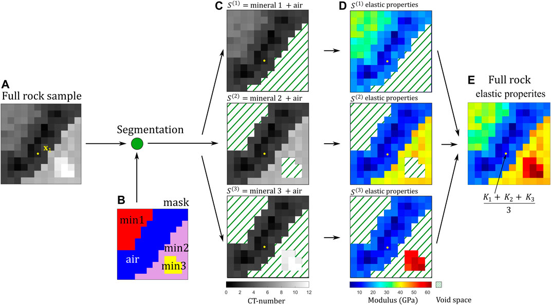
FIGURE 6. The diagram of the modified-SLOT. Here, we show an example of a two-dimensional section of a rock sample consisting of three mineral phases (A). In the CT-volume, the domain is discretized on a uniform grid depending on the resolution of the scan. The first step of the modified-SLOT is to partition the domain into small subdomains ($S^{\left(1\right)}, S^{\left(2\right)},$ and $S^{\left(3\right)}$) using the segmentation mask (B). Each subdomain consists of two phases: a mineral phase and the air phase (C). Next, since the subdomains are monomineralic, we apply the SLOT to each subdomain, transforming the CT-volumes in the elastic properties volumes (D). Finally, we combine each subdomain, getting back the full volume elastic properties volume. In the figure, ${\mathbf{x}}_1$ is located in the air phase. The elastic properties at ${\mathbf{x}}_1$ in the full volume is the average of the elastic properties from each subdomain (i.e., $\left(K_1+K_2+K_3\right)/3$) (E).

The last step of the modified-SLOT is to recombine all subdomains elastic property maps, obtaining an elastic properties model of the full sample. The processes to recombine minerals and pores are different. For minerals, the elastic properties of the voxels in the subdomain and in the recombined volume are the same. For pores, the elastic properties in the recombined volume are computed as the arithmetic average of the voxel elastic properties in all the subdomains. For example, in a polymineralic rock with three minerals, a voxel that is located at ${\mathbf{x}}_1$ is classified as air (i.e., pore space) (Figures 6A,B). The partitioning step copies this voxel into three subdomains (Figure 6C). The SLOT algorithm will assign to such a voxel a slightly different elastic modulus in each subdomain ($K_1,K_2$, and $K_3$) (Figure 6D). $K_1,K_2$, and $K_3$ values are slightly different from one another due to the different parameters used by the SLOT in each subdomain. When the voxel is recombined to the full sample elastic properties model, the modulus of ${\mathbf{x}}_1$ will be $(K_1+K_2+K_3)/3$ (Figure 6E).

Estimating Sub-Resolution Pore Space in Each Subdomain

When the rock sample contains only two-minerals, the sub-resolution porosity in each subdomain $\left({\mathit{f}}_{\mathbf{p}\mathbf{o}\mathbf{r}\mathbf{e}1}\text{and }{\mathit{f}}_{\mathbf{p}\mathbf{o}\mathbf{r}\mathbf{e}2}\right)$ can be computed from the measured porosity (ϕ_lab), the density of the sample (${\rho }_{\text{lab}}$), and the segmented CT-images.

The segmentation described in the previous section provides approximations for 1) the volume fraction of mineral 1 ($f_1^{\text{seg}}- {\mathit{f}}_{\mathbf{p}\mathbf{o}\mathbf{r}\mathbf{e}1}$), 2) the volume fraction of mineral 2 ($f_2^{\text{seg}}- {\mathit{f}}_{\mathbf{p}\mathbf{o}\mathbf{r}\mathbf{e}2}$), and 3) the volume fraction of air $\left(f_{\text{air}}^{\text{seg}}\right)$. $f_1^{\text{seg}}$ and $f_2^{\text{seg}}$ comprises S⁽¹⁾ and S⁽²⁾, respectively, and unknown amounts of sub-resolution pore space that here we call $f_{\text{pore}1}$ and $f_{\text{pore}2}$ - i.e., the unknown volume fractions of sub-resolution pore space in $f_1^{\text{seg}}$ and $f_2^{\text{seg}}$, respectively. Thus, the density of the CT-imagery is:

where ${\rho }_1, {\rho }_2$, and ${\rho }_{air}$ are the densities of the mineral comprised of S⁽¹⁾, S⁽²⁾, and air, respectively. Moreover, the estimated porosity from the CT-volume is:

If we assume that the CT-volume is a representative sample, the density obtained from Eq. 2 and the porosity obtained from Eq. 3 are equivalent to ${\rho }_{\text{lab}}$ and ${\varphi }_{\text{lab}}$, respectively. Solving the system of two equations yields $f_{\text{pore}1}$ and $f_{\text{pore}2}$. Thus, the porosity of the two subdomains are:

Remember that the total porosity of the sample, ϕ_lab, is defined as the ratio of the void space over the total volume of the sample. On the other hand, ${\varphi }_{\text{lab}}^{\left(1\right)}$ and ${\varphi }_{\text{lab}}^{\left(2\right)}$, are the ratio of the void space over the subdomain volumes, which are smaller than the total volume of the sample. Therefore, the values of ${\varphi }_{\text{lab}}^{\left(1\right)}$ and ${\varphi }_{\text{lab}}^{\left(2\right)}$ are greater than ϕ_CT and ϕ_lab.

Evaluating Effective Elastic Properties of the Sample

We used Elas3D to estimate the elastic properties of sample B. “Elas3D” is a numerical code written in Fortran 77 by the National Institute of Standards and Technology (Garboczi, 1998). Such a code uses finite element methods to solve the linear elastic equation on a discrete domain with a cubic mesh. The code solves the equation:

where σ is the stress tensor, f is the body force, and $\nabla \cdot$ is the divergence operator. Equation 5 is subjected to the prescribed strain boundary condition:

where ${\mathrm{ϵ}}_0$ is the prescribed strain tensor at the domain boundary. In this study, we apply a strain boundary condition of ${\mathrm{ϵ}}_0=\mathit{ }\left[1.0, 1.0, 1.0, 0.5, 0.5, 0.5\right]$ to the sample (Voigt’s notation). Note that solving Eq. 5 and Eq. 6 is equivalent to the energy minimization problem:

where $\mathbf{C}$ is the elastic properties tensor and : denotes the inner tensor product (dot product). The elas3D code is implemented with a periodic boundary condition. Given the elastic properties of a material at each voxel and the prescribed strain magnitude at the boundaries, the code numerically solves Eqs 5–7 for the stress tensor at each element with the conjugate gradient algorithm. Then, effective elastic properties are calculated with the average stress and the average strain. Using Voigt’s notation, let σ_i(x,y,z) and ϵ_i(x,y,z) denote the ith component of the stress and the strain tensor at (x,y,z), respectively. Assuming that the sample is isotropic, the effective Bulk modulus K_eff, and the effective shear modulus G_eff, of the sample are:

where $\text{Σ}$ denoted the sum over the entire domain. The effective Young’s modulus is computed as:

Segmentation-Based DRP

We also created and tested a segmented model to compare a segmentation-based DRP approach to our proposed technique. In the segmentation-based DRP, voxels are categorized based on the CT-number. The voxels are then assigned with the elastic properties of the pristine material. For example, a voxel that had been identified as the calcite would have the bulk modulus of 65 GPa and shear modulus of 32 GPa (Table 3). Each voxel is associated with only one material. To create our segmented model, we use the simple-threshold method, where a cut-off CT-number is defined to separate different phases. Here, the cut-off CT-number is chosen so that the digital sample porosity equals ${\varnothing }_{\text{lab}}$.

Parameters and Assumptions

To compute the sub-resolution porosity, we assumed that the sample contains only two mineral phases: dolomite and calcite. Voxels that were classified as heavy minerals were grouped alongside calcite. To verify that such an approximation did not significantly affect the final effective modulus of the sample, we compared the Young’s moduli of two samples calculated through the Voigt-Reuss-Hill average (Hill, 1963). The first sample comprised 8.65% pore space, 69.17% calcite, 22.13% dolomite, and 0.05% heavy mineral (i.e., the volumetric fractions estimated via segmentation). The second sample comprised of 8.65% pore space, 69.22% calcite, and 22.13% dolomite. We then assumed that the heavy mineral was pyrite (one of the most rigid and stiff heavy minerals) with bulk and shear modulus of 147 GPa and 132 GPa, respectively. The absolute difference between the two estimated Young’s moduli was 0.2% (i.e., 41.5 vs. 41.4 GPa), suggesting that a sample comprising only dolomite and calcite was a good proxy for our sample.

The pore aspect ratio of the sub-resolution porosity, that was an input parameter for the modified-DEM, was estimated from the TOMCAT dataset using AVIZO 9.0 (Avizo, 2019) with the following workflow. First, pore space was segmented from the images with the AVIZO thresholding tool. Then, we applied the watershed algorithm (Separate Object command in AVIZO) to label each pore. We then computed the aspect ratio of each pore with the Label Analysis tool. Finally, the weighted harmonic average of the aspect ratios of all the pores was computed. Such an estimate yielded a pore aspect ratio of 0.47. Nonetheless, to account for uncertainties, we computed the elastic properties of sample B for aspect ratio end-members of 0.4 and 0.5. Note that the higher the aspect ratio, the higher the effective elastic properties.

To convert CT-numbers to density, we used a linear calibration. Such a procedure is described in detail in the Supplementary Information. In the density-to-porosity conversion, the cut-off densities (${\rho }_0$) for the two subdomains ($S_{\text{dol }}^{\left(1\right)}$ and $S_{\text{cal }}^{\left(2\right)}$) were the density of dolomite (2870 kg/m³) and calcite (2710 kg/m³), respectively. The elastic properties used in the modified-DEM are given in Table 3. We assumed a critical porosity for both subdomains of 0.40, which is a typical value for carbonate rocks (Nur et al., 1998; Fournier et al., 2018).

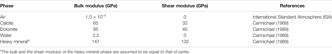
TABLE 3. Elastic properties of minerals and air.

Results

Laboratory Results

Attenuation curves (Figure 7) reveal that for both cases, dry and full saturation (100%), attenuation ranges between 0 and 0.03 and increases with increasing frequency. Young’s modulus patterns show dispersion in each case in agreement with a non-zero attenuation. At 5 MPa confining pressure and frequencies between 1 and 5 Hz, the average Young’s modulus are 23.8 ± 0.1 GPa and 29.4 ± 0.1 GPa for the dry and 100% water-saturated case, respectively. It can also be observed that the saturated sample presents an increased values of the Young’s modulus as predicted by the Gassmann theory (Gassmann, 1951).

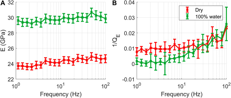
FIGURE 7. Laboratory measurements of Young’s modulus (E) and attenuation (1/Q_E) for the carbonate under dry conditions and full saturation (100%) with water (1 cP) at confining pressures of 5 MPa.

DRP Results

Modified-SLOT on the Sample

According to the segmented CT-volume, the super-resolution porosity is 8.65%. The segmented volumes fraction of the first mineral (dolomite) and the second mineral (calcite) are $f_1^{\text{seg}}=0.2213$ and $f_2^{\text{seg}}=0.6922$, respectively. We substitute ${\rho }_{\text{lab}}$ and ϕ_lab into Eqs 2–4 and perform the optimization process, this gives the porosity volumes of the two subdomains equal to ${\varphi }_{\text{CT}}^{\left(1\right)}=$ 0.294 and ${\varphi }_{\text{CT}}^{\left(2\right)}=$ 0.192, respectively (Figure 8). Recombination yields a porosity for the entire sample ${\varphi }_{\text{CT}}=$ 0.1535, which is 0.97% lower than ϕ_lab. The five sub-volumes extracted from sample F have porosities ranging between 0.1427 and 0.1669 (Table 3).

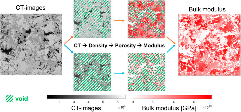
FIGURE 8. A schematic diagram of the modified-SLOT on the sample. The sample is partitioned into two subdomains. The dolomite subdomain $\left(S_{\text{dol}}^{\left(1\right)}\right)$ is shown in the bottom row and the calcite subdomain $\left(S_{\text{cal}}^{\left(2\right)}\right)$ is shown in the top row. Notice that the air phases in both samples are the same.

Young’s Modulus from Numerical Simulations

The five sub-volume Young’s moduli that were computed from the modified-SLOT range between 22.6 and 29.2 GPa and from 25.1 to 31.5 GPa for aspect ratio of 0.4 and 0.5, respectively (Table 1). On average, the predicted Young’s modulus is 26.1 ± 1.7 GPa and 28.7 ± 1.9 GPa for the dry case and the water-saturated case, respectively. The fifth sub-volume, which has the closest porosity to the laboratory-measured porosity, yields Young’s modulus of 25.6 GPa and 26.9 GPa for aspect ratio of 0.4 and 0.5 scenarios, respectively. The results suggest that, in the worst-case scenario, the calculated Young’s modulus of the sample computed with aspect ratio of 0.5 would give 13% higher than the laboratory-measured Young’s modulus. We observe a similar trend in the 100% water-saturated case. On the fifth sub-volume with the simulation aspect ratio of 0.5, Young’s modulus obtained from modified-SLOT is 30.5 GPa, which is 4.1% higher than the laboratory measurement at 1 Hz. Instead, Young’s modulus predicted from the segmentation-based DRP overpredicts the laboratory-measured Young’s modulus by 180% and 140% for the dry and the water-saturated case, respectively. Table 1 and Figure 9 summarize the numerical simulation results from the modified-SLOT.

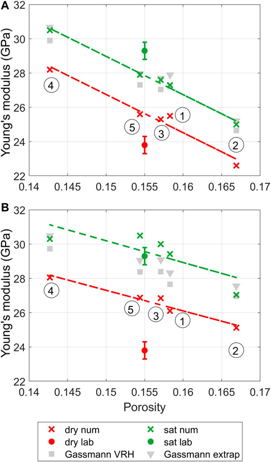
FIGURE 9. The comparison between the laboratory-measured and the numerical simulated Young’s modulus. Here, we show the result from two scenario: simulation with aspect ratio of 0.4 (A) and aspect ratio if 0.5 (B). The dry case and the 100% water-saturated case are represented in red and green, respectively. Five numerical simulations on sub-volumes are shown with the cross symbol, and the sub-volume numbers are labeled next to the cross symbol. We fit the first-order polynomial through the numerical simulation results, observing a decreasing trend between the Young’s modulus and the porosity. The gray triangle and square symbols represent the estimated Young’s modulus using Gassmann’s equation. The mineral modulus is approximated with the linear extrapolation of the sub-volume modulus (triangle symbols) and the Voight-Reuss-Hill average (square symbols).

Discussion

Microporosity Estimation

Roughly 40% of the porosity of our sample is not detectable from the ETH-dataset. The amount of sub-resolution porosity agrees with the literature on similar lithologies (e.g., Sok et al., 2010; Lin et al., 2016) and the MICP test. The distribution of sub-resolution porosity cannot be estimated using the segmentation-based DRP on CT-images. As such, we suggest that the segmentation-less DRP is a more suitable technique. Note that the aspect ratio of pores could be estimated from the MICP data and the CT-images. Future research should focus on improving the estimate of pore aspect ratios.

Static Young’s Modulus Estimation

The static Young’s modulus that is computed from the numerical simulations is a proxy for the zero-frequency limit of the laboratory measured Young’s modulus measured in the laboratory. Nonetheless, the overprediction of the modulus might come from the type of boundary conditions that we used in the simulation. Here, the numerical code prescribes strain boundary conditions. The strain boundary condition gives the upper bound of the effective modulus if the size of the sample is not representative (Ostoja-Starzewski, 1999). On the other hand, the stress boundary condition gives the lower bound under the same condition. Hence, the numerical predicted modulus might give the upper limit of the Young’s modulus instead of the actual modulus of the sample that was measured by applying stress boundary conditions.

The static Young’s moduli that we obtained from the modified-SLOT are more precise than those from the segmentation-based DRP. We speculate that such an improvement is due to the material-mixing strategy, creating a more realistic and flexible model (Tisato and Spikes, 2016). In addition, the improvement is also from the ability of the modified-SLOT to account for the effect of microporosity on the elastic properties.

In the segmentation-based DRP, the predicted Young’s modulus overestimates the laboratory-measured result by 180% even though the porosity of the model matches ϕ_lab. This observation suggests that the spatial distribution of the pore space does affect the effective Young’s modulus of the sample. Note that the simple threshold-based segmentation method has been shown to be ineffective for computing elastic properties of carbonate rocks (e.g., Madonna et al., 2012; Andrä et al., 2013b; Saenger et al., 2016; Sun et al., 2017). Therefore, we also conclude that the threshold-based segmentation is not a suitable technique for rocks with complex mineralogy and pore structures.

The successful result using modified-SLOT implies that we could have used the same strategy with the SLIT if we had physical targets scanned along with the sample. Such a method could have spared the measurement of porosity from the laboratory. In the worst-case scenario where the simulations are performed with aspect ratio of 0.5, the average error in Young’s modulus computed from the modified-SLOT is 9.9%, which implies an error on the extensional wave velocity of 4.8%. An error of ∼5% on wave velocities is similar to that yielded by the SLOT method that was applied on a Berea sandstone sample (Ikeda et al., 2020). We know the precision but not the accuracy of our laboratory measurements. Nevertheless, we can assume that accuracy for our laboratory measurements is around ±7%, which is similar to the uncertainty of the modified-SLOT.

Young’s Modulus Prediction from Effective Medium Theories

The effective Young’s modulus of the rock could also be estimated using theoretical models. We compare the effective Young’s modulus of the fifth sub-volume obtained from the numerical simulation and EMTs, applied to the entire sample. The composition of the fifth sub-volume, estimated from the modified-SLOT, is 20.7% dolomite, 63.8% calcite, and 15.4% air. Dolomite has 0.35% of sub-resolution pore space, and calcite has 7.20% of sub-resolution pore space. Overall the sample has 7.85% super-resolution pore space. We consider the dry case and three EMTs to estimate Young’s modulus of the sample: 1) Voigt-Reuss-Hill average (Hill, 1963), 2) average Hashin-Shtrikman bounds (Hashin and Shtrikman, 1963), and 3) modified-DEM. The latter provides a comparison between the modified-SLOT, where the modified-DEM is applied to each voxel, and the modified-DEM applied on the entire sample. Unfortunately, the modified-DEM is only applicable to a rock with two minerals. Thus, we estimate the Young’s modulus of the sample using the modified-DEM with a mixture material strategy as follow. First, we define two new phases: the porous dolomite phase and the porous calcite phase. The modulus of the porous dolomite phase, $M_{\text{dol}}$, is computed by mixing dolomite with penny shaped inclusions whose aspect ratio is 0.4. The volume fraction of the inclusions is 0.35%. Similarly, the modulus of the porous calcite phase, $M_{\text{cal}}$, is computed by mixing calcite to penny shaped pores having aspect ratio 0.4 and volume fraction 7.20%. These inclusion volume fractions are equal to the missing porosity in each subdomain. Then, the mixed moduli are computed from the modified-DEM where the critical porosity is 0.40. Next, the modulus of the sample -i.e., the mixture of the porous calcite and dolomite - is obtained from the Voigt-Reuss-Hill average.

The Young’s modulus of the sample computed from Voigt-Reuss-Hill average, average Hashin-Shtrikman bounds, and modified-DEM are 38.4 GPa, 33.9 GPa, and 30.5 GPa, respectively. Such estimates are approximately 44% higher than the laboratory-measured Young’s modulus. EMTs overestimate elastic properties because they do not incorporate the spatial distribution of phases and the geometry of grains and pores.

Gassmann Fluid Substitution on DRP

The Young’s modulus of the 100% water-saturated sample from the numerical simulation mostly agrees with Gassmann fluid substitution. Figure 9 shows a comparison between all the numerical simulations (green dots) and the algebraically estimated Young’s modulus (gray dots). We also show the results on both simulation scenarios: aspect ratio of 0.4 and 0.5 (Figures 9A,B). The algebraically estimated Young’s modulus is computed by directly applying Gassmann’s fluid substitution to the dry bulk and shear modulus, porosity, mineral fraction, and mineral modulus (usually refer as $K_0$) of each sub-volume. The mineral modulus is estimated in two ways. The first method approximates the mineral modulus by computing the Voigt-Reuss- Hill average of the mineral constituents (square symbol in Figure 9). The second method finds $K_0$ by linearly extrapolating the dry bulk modulus of the sample at zero porosity. Both methods yield similar results except for sample sub-volume 1, 3, and 5 in the aspect ratio of 0.5 simulations (Figure 9B).

The fluid substituted Young’s modulus computed from the modified-SLOT underestimates the laboratory measurement. The results from the laboratory measurement suggest a 23% increase in Young’s modulus when the sample is fully saturated. On the other hand, Gassman predicts that the average increment in Young’s modulus should be 9.7%. A similar modulus mismatch between the Gassmann prediction and the laboratory measurement for carbonate samples has been reported in the literature (e.g., Marion and Jizba, 1997; Wang, 1997; Røgen et al., 2005). These discrepancies imply that the Gassmann fluid substitution does not provide accurate results for this type of rock. We hypothesize that some reasons could be:

• During the saturation process in the laboratory, chemical interaction between pore fluid and rock frame altered the elastic properties of the rock (e.g., Assefa et al., 2003; Baechle et al., 2005);

• Compliant pore spaces (aspect ratio of ∼0.4–0.5) in the sample might introduce anisotropic behaviors (Adam et al., 2006); hence, the isotropic Gassman substitution equation might not be valid; and,

• As previously mentioned, the laboratory measurement of Young’s modulus has an error ∼7%.

Another source of uncertainty is related to the boundary conditions. The laboratory experiment was performed under drained conditions. The numerical simulation, on the other hand, is performed under undrained condition and the modulus computed under the undrained condition is expected to be higher than that in the drained condition. Therefore, further investigation is needed for a more suitable model to simulate the elastic properties of rocks at drained water-saturated conditions.

Size of the Sample in the Numerical Simulation

We would like to emphasize that due to limitations on computational resources, the numerical simulations are performed on sub-volumes smaller than the core used in laboratory measurements. We assume that the numerical simulation on the small sample is still a proxy for the laboratory-sized sample. We consider the lithology understudy to have a low heterogeneity degree. Such an assumption is partially supported by the fact that sample C, D and E have similar measured porosity.

Nevertheless, the size of REVs depends on the heterogeneity level of the lithology. Rozenbaum and Roscoat (2014) studied REVs of CT-images of carbonate samples. They found that a sub-volume of size ∼3 mm³ is considered to be a representative size for calculating the porosity of limestone. Araújo et al. (2018), on the other hand, suggested that sub-volumes of size ∼10 mm³ could be used to compute porosities effectively. Nonetheless, the physical properties of the sub-volumes still depend on the location where the sub-volumes are extracted. Therefore, we cannot certainly conclude that the subsamples used in the numerical simulations are REVs for the sample. Nonetheless, the purpose of this manuscript is to demonstrate the possibility of using the segmentation-less DRP on polymineralic samples and achieve an improvement over the segmentation-based DRP. Future study is required to simulate the numerical tests on a larger rock sample. Such additional tests will be more efficiently performed on shared memory cluster systems and a parallelized version of elas3D using, for instance, OpenMPI (Bohn and Garboczi, 2003).

The Effect of Phase Segmentation

The modified-SLOT uses a segmentation algorithm to separate different phases. In our study, we used a simple threshold-based algorithm. Nevertheless, other algorithms could be chosen, introducing uncertainty in the final results as different segmentation algorithms could potentially lead to different rock models (e.g., Andrä et al., 2013a). Here, we consider the uncertainty related to the threshold-based segmentation method in segmenting the air phase. We suppose that an x fraction of dolomite voxels, due to the segmentation threshold, is classified as air. We can write:

The porosity of the segmentation-based model will increase by x. On the other hand, the porosity of the model created from the modified-SLOT, will increase only by a fraction of x. For example, if x = 0.05, solving Eqs 2–5 gives ${\varphi }_{\text{lab}}^{\left(1\right), \text{new}}=0.298$ and ${\varphi }_{\text{lab}}^{\left(2\right), \text{new}}=0.197$, which are ∼0.3% and ∼2% greater than the porosities obtained in the original model. Then, when we apply the SLOT optimization process, the effective porosity of sample F is estimated to be 0.159, which is 1.3% higher than the original estimated porosity. Using different thresholds, we obsevere an increase in porosity of 0% (no change) and 2.6% when x = 0.01 and x = 0.1, respectively. Such limited analysis suggests that the modified-SLOT is less sensitive to the threshold level compared to the segmentation-based DRP. Future investigation is needed to study how the segmentation algorithm and parameters affect the final result: elastic properties of materials. And, we need to investigate the effect of the segment threshold on the other phases.

Possible Applications

Segmentation-less DRP allows capturing sub-resolution features without having to scan a sample at nanometric resolutions (i.e., segmentation-based DRP). The low-resolution scan (microns) covers a larger portion of the sample, which are likely to be REVs of formations (e.g., Lai et al., 2017; Hertel et al., 2018). Hence, such a scan could be used to compute properties of samples, served as a first-order approximation for further analysis.

Since the modified-SLOT relaxes the monomineralic assumption of the current segmentation-less DRP workflows, numerical simulations could be performed on a wide variety of rocks such as limestone and lithic sandstone. The EMT needs to be adjusted according to the sample lithology (e.g., grain packing model for clastic rocks). Incorporating EMTs to DRP also allows us to combine theoretical rock physics templates with digital rock physics simulations, giving the possibilities of investigating the impact of different rock physics models on rocks’ properties. Note that the procedure could also be used to compute petrophysical properties other than elastic properties. For example, we can use the Hashin-Shtrikman bounds of electrical conductivity with modified-SLOT to create a conductivity model (Hashin and Shtrikman, 1963; Waff, 1974; Brovelli and Cassiani, 2010). Further studies are needed to test the validity of the concept.

Conclusion

We have introduced the modified-SLOT, a new digital rock physics technique, to evaluate the elastic properties of polymineralic rocks. The modified-SLOT combines segmentation-based DRP to reconstruct the spatial distribution of mineral phases, and segmentation-less DRP to account for the effect of sub-resolution features. Segmentation partitions a polymineralic rock sample into smaller subsamples that are monomineralic. Then, segmentation-less converts CT-images into density, porosity, and elastic property arrays. DRP results were compared to low-frequency measurements of Young’s modulus on a polymineralic carbonate sample. The modified-SLOT provides a more accurate prediction of Young’s modulus over the segmentation-based DRP. Such an improvement is because the modified-SLOT can capture the effect of microporosity on the sample elastic properties. Thus, modified-SLOT provides more realistic models for numerical simulations. Nonetheless, the modified-SLOT still inherits the segmentation-based DRP uncertainties in choosing segmentation algorithms. Future works need to be focused on assessing the uncertainties arising from the choice of segmentation algorithms. Although the modified-SLOT needs the information about the porosity of the samples, the success of modified-SLOT implies that a similar technique could be used when phantoms are presented in the scan (i.e., SLIT). Hence, the modified-SLOT and modified-SLIT could be used as a first-order proxy for predicting petrophysical properties of samples, cores, or cuttings, assisting geoscientists in creating fast and accurate subsurface models using X-ray CT technology.

Data Availability Statement

The datasets presented in this article are not readily available because CT-scan data are proprietary. All the other data are sharable. Requests to access the datasets should be directed to Ken Ikeda, ikeda.ken@utexas.edu

Author Contributions

The laboratory experiment was performed by SS, BQ, and ES. Digital Rock Physics and data analysis were performed by KI, EG, and NT. The preparation of the manuscript, including figures and tables were led by KI, under the supervision of NT. SS, BQ, ES, and EG assisted in the preparation process.

Funding

The first-author of the manuscript, KI, was funded by the EDGER Forum, The University of Texas at Austin. The AVIZO program and computer resources were supported by NSF grant EAR-1762458 to the University of Texas High-Resolution X-ray Computed Tomography Facility.

Conflict of Interest

The authors declare that the research was conducted in the absence of any commercial or financial relationships that could be construed as a potential conflict of interest.

Supplementary Material

The Supplementary Material for this article can be found online at: https://www.frontiersin.org/articles/10.3389/feart.2021.628544/full#supplementary-material.

Acknowledgments

We would like to thank Michael Plötze for performing X-ray computed tomography of the sample and the MICP measurement at the claylab of ETH Zürich, Switzerland. Access to AVIZO and computer resources, used to run AVIZO, were supported by NSF grant EAR-1762458 to the University of Texas High-Resolution X-ray Computed Tomography Facility. We would also want to thank the editor and the reviewers for suggestions on the manuscript. The datasets presented in this article are not readily available because CT-scan data are proprietary. All the other data are sharable. Requests to access the datasets should be directed to the corresponded author. Code for the SLOT is available at https://github.com/ikedatu72/SegmentaionLessW-OTarget. The information on the numerical simulation solver is available at https://github.com/ikedatu72/elas3D-python.

References

Adam, L., Batzle, M., and Brevik, I. (2006). Gassmann’s fluid substitution and shear modulus variability in carbonates at laboratory seismic and ultrasonic frequencies. Geophysics. 71 (6), F173–F183. doi:10.1190/1.2358494
AlJallad, O., Dernaika, M., Koronfol, S., Naseer Uddin, Y., and Mishra, P. (2020). “Evaluation of complex carbonates from pore-scale to core-scale,” in International petroleum technology conference, January 13–15, 2020, Dhahran, Kingdom of Saudi Arabia.
Amabeoku, M. O., Al-Ghamdi, T. M., Mu, Y., Ingrain, R., and Toelke, J. (2013). Evaluation and application of digital rock physics (DRP) for special core analysis in carbonate formations.
Andrä, H., Combaret, N., Dvorkin, J., Glatt, E., Han, J., Kabel, M., et al. (2013a). Digital rock physics benchmarks—part I: imaging and segmentation. Comput. Geosci. 50, 25–32. doi:10.1016/j.cageo.2012.09.005
Andrä, H., Combaret, N., Dvorkin, J., Glatt, E., Han, J., Kabel, M., et al. (2013b). Digital rock physics benchmarks—part II: computing effective properties. Comput. Geosci. 50, 33–43. doi:10.1016/j.cageo.2012.09.008
Araújo, O., Sharma, K., Machado, A., Ferreira, C. G., Straka, R., Tavares, F., et al. (2018). Representative elementary volume in limestone sample. J. Instrum. 13, C10003. doi:10.1088/1748-0221/13/10/C10003
Assefa, S., McCann, C., and Sothcott, J. (2003). Velocities of compressional and shear waves in limestones. Geophys. Prospect. 51 (1), 1–13. doi:10.1046/j.1365-2478.2003.00349.x
Avizo (2019). [Computer software]. Thermo fisher scientific. Available at: https://www.thermofisher.com/ (Version 9). (Accessed December 1, 2020)
Baechle, G. T., Weger, R. J., Eberli, G. P., Massaferro, J. L., and Sun, Y.-F. (2005). Changes of shear moduli in carbonate rocks: implications for Gassmann applicability. Lead. Edge. 24 (5), 507–510. doi:10.1190/1.1926808
Baumgartner, R. J., Kranendonk, M. J. V., Wacey, D., Fiorentini, M. L., Saunders, M., Caruso, S., et al. (2019). Nano−porous pyrite and organic matter in 3.5-billion-year-old stromatolites record primordial life. Geology. 47 (11), 1039–1043. doi:10.1130/G46365.1
Bohn, R. B., and Garboczi, E. J. (2003). NIST Interagency/Internal Report (NISTIR) – 6997. User manual for finite element and finite difference programs: a parallel version of NISTIR 6269 and NISTIR 6997. Available at: https://www.nist.gov/publications/user-manual-finite-element-and-finite-difference-programs-parallel-version-nistir-6269 (Accessed December 25, 2020).
Brovelli, A., and Cassiani, G. (2010). A combination of the Hashin-Shtrikman bounds aimed at modelling electrical conductivity and permittivity of variably saturated porous media. Geophys. J. Int. 180 (1), 225–237. doi:10.1111/j.1365-246X.2009.04415.x
Buades, A., Coll, B., and Morel, J.-M. (2005). “A non-local algorithm for image denoising,” in IEEE computer society conference on computer vision and pattern recognition (CVPR’05) Vol. 2, 60–65.
Carmichael, R. S. (1989). Practical handbook of physical properties of rocks and minerals. Boca Raton, Fla: CRC Press.
Chafetz, H., Barth, J., Cook, M., Guo, X., and Zhou, J. (2018). Origins of carbonate spherulites: implications for Brazilian Aptian pre-salt reservoir. Sediment. Geol. 365, 21–33. doi:10.1016/j.sedgeo.2017.12.024
Chantler, C. T., Olsen, K., Dragoset, R. A., Chang, J., Kishore, A. R., Kotochigova, S. A., et al. (2005). X-Ray form factor, attenuation and scattering tables. National Institute of Standards and TechnologyAvailable at: http://physics.nist.gov/ffast, Version 2.1. (Accessed November 15, 2020)
Dunsmuir, J. H., Bennett, S., Fareria, L., Mingino, A., and Sansone, M. (2006). X-ray microtomographic imaging and analysis for basic research. Powder Diffr. 21 (2), 125–131. doi:10.1154/1.2204956
Fournier, F., Pellerin, M., Villeneuve, Q., Teillet, T., Hong, F., Poli, E., et al. (2018). The equivalent pore aspect ratio as a tool for pore type prediction in carbonate reservoirs. AAPG Bull. 102 (7), 1343–1377. doi:10.1306/10181717058
Garboczi, E. J. (1998). NIST interagency/internal report (NISTIR) – 6269. Finite element and finite difference programs for computing the linear electric and elastic properties of digital images of random materials | NIST. Available at: https://www.nist.gov/publications/finite-element-and-finite-difference-programs-computing-linear-electric-and-elastic (Accessed November 15, 2020).
Gomes, J. P., Bunevich, R. B., Tedeschi, L. R., Tucker, M. E., and Whitaker, F. F. (2020). Facies classification and patterns of lacustrine carbonate deposition of the Barra Velha Formation, Santos Basin, Brazilian Pre-salt. Mar. Petrol. Geol. 113, 104176. doi:10.1016/j.marpetgeo.2019.104176
Gupta, L. P., Tanikawa, W., Hamada, Y., Hirose, T., Ahagon, N., Sugihara, T., et al. (2018). Examination of gas hydrate-bearing deep ocean sediments by X-ray Computed Tomography and verification of physical property measurements of sediments. Marine Pet. Geol. 108, 239–248. doi:10.1016/j.marpetgeo.2018.05.033
Han, J., Han, S., Kang, D. H., Kim, Y., Lee, J., and Lee, Y. (2020). Application of digital rock physics using X-ray CT for study on alteration of macropore properties by CO2 EOR in a carbonate oil reservoir. J. Petrol. Sci. Eng. 189, 107009. doi:10.1016/j.petrol.2020.107009
Hashin, Z., and Shtrikman, S. (1963). A variational approach to the theory of the elastic behaviour of multiphase materials. J. Mech. Phys. Solid. 11 (2), 127–140. doi:10.1016/0022-5096(63)90060-7
Hertel, S. A., Rydzy, M., Anger, B., Berg, S., Appel, M., and de Jong, H. (2018). “Upscaling of digital rock porosities by correlation with whole core CT Scan Histograms,” in SPWLA 59th annual logging symposium.
Hill, R. (1963). Elastic properties of reinforced solids: some theoretical principles. J. Mech. Phys. Solid. 11 (5), 357–372. doi:10.1016/0022-5096(63)90036-X
Iassonov, P., Gebrenegus, T., and Tuller, M. (2009). Segmentation of X-ray computed tomography images of porous materials: a crucial step for characterization and quantitative analysis of pore structures. Water Resour. Res. 45 (9), W09415. doi:10.1029/2009WR008087
Ikeda, K., Goldfarb, E., and Tisato, N. (2020). Calculating effective elastic properties of Berea Sandstone using the segmentation-less method without targets. J. Geophys. Res.: Solid Earth 125, e2019JB018680. doi:10.1029/2019JB018680
Ketcham, R., and Carlson, W. D. (2001). Acquisition, optimization and interpretation of X-ray computed tomographic imagery: applications to the geosciences. Comput. Geosci. 27, 381–400. doi:10.1016/S0098-3004(00)00116-3
Lai, J., Wang, G., Fan, Z., Chen, J., Qin, Z., Xiao, C., et al. (2017). Three-dimensional quantitative fracture analysis of tight gas sandstones using industrial computed tomography. Sci. Rep. 7, 1825. doi:10.1038/s41598-017-01996-7
Lin, Q., Al-Khulaifi, Y., Blunt, M. J., and Bijeljic, B. (2016). Quantification of sub-resolution porosity in carbonate rocks by applying high-salinity contrast brine using X-ray microtomography differential imaging. Adv. Water Resour. 96, 306–322. doi:10.1016/j.advwatres.2016.08.002
Madonna, C., and Tisato, N. (2013). A new Seismic Wave Attenuation Module to experimentally measure low-frequency attenuation in extensional mode: a seismic wave attenuation module to measure low-frequency attenuation. Geophys. Prospect. 61 (2), 302–314. doi:10.1111/1365-2478.12015
Madonna, C., Almqvist, B. S. G., and Saenger, E. H. (2012). Digital rock physics: numerical prediction of pressure-dependent ultrasonic velocities using micro-CT imaging. Geophys. J. Int. 189 (3), 1475–1482. doi:10.1111/j.1365-246X.2012.05437.x
Marion, D., and Jizba, D. (1997). “5. Acoustic properties of carbonate rocks: use in quantitative interpretation of sonic and seismic measurements,” in Carbonate seismology. (Tulsa, OK: Society of Exploration Geophysicists), Vol. 1, 75–94.
Mavko, G., Mukerji, T., and Dvorkin, J. (2020). The rock physics handbook. 3rd Edn. Cambridge: Cambridge University Press.
Mukerji, T., Berryman, J., Mavko, G., and Berge, P. (1995). Differential effective medium modeling of rock elastic moduli with critical porosity constraints. Geophys. Res. Lett. 22 (5), 555–558. doi:10.1029/95GL00164
Mull, R. T. (1984). Mass estimates by computed tomography: physical density from CT numbers. AJR Am. J. Roentgenol. 143 (5), 1101–1104. doi:10.2214/ajr.143.5.1101
Nock, R., and Nielsen, F. (2004). Statistical region merging. IEEE Trans. Pattern Anal. Mach. Intell. 26 (11), 1452–1458. doi:10.1109/TPAMI.2004.110
Norris, A. N., Callegari, A. J., and Sheng, P. (1985). A generalized differential effective medium theory. J. Mech. Phys. Solid. 33 (6), 525–543. doi:10.1016/0022-5096(85)90001-8
Nur, A., Mavko, G., Dvorkin, J., and Galmudi, D. (1998). Critical porosity: a key to relating physical properties to porosity in rocks. Lead. Edge. 17 (3), 357–362. doi:10.1190/1.1437977
Ostoja-Starzewski, M. (1999). Scale effects in materials with random distributions of needles and cracks. Mech. Mater. 31 (12), 883–893. doi:10.1016/S0167-6636(99)00039-3
Paterson, M. S., and Olgaard, D. L. (2000). Rock deformation tests to large shear strains in torsion. J. Struct. Geol. 22, 1341–1358. doi:10.1016/S0191-8141(00)00042-0
Røgen, B., Fabricius, I. L., Japsen, P., Høier, C., Mavko, G., and Pedersen, J. M. (2005). Ultrasonic velocities of North Sea chalk samples: influence of porosity, fluid content and texture. Geophys. Prospect. 53 (4), 481–496. doi:10.1111/j.1365-2478.2005.00485.x
Rozenbaum, O., and du Roscoat, S. R. (2014). Representative elementary volume assessment of three-dimensional x-ray microtomography images of heterogeneous materials: application to limestones. Phys. Rev. E – Stat. Nonlinear Soft Matter Phys. 89, 053304. doi:10.1103/PhysRevE.89.053304
Saenger, E. H., Vialle, S., Lebedev, M., Uribe, D., Osorno, M., Duda, M., et al. (2016). Digital carbonate rock physics. Solid Earth 7 (4), 1185–1197. doi:10.5194/se-7-1185-2016
Schindelin, J., Arganda-Carreras, I., Frise, E., Kaynig, V., Longair, M., Pietzsch, T., et al. (2012). Fiji: an open-source platform for biological-image analysis. Nat. Methods. 9 (7), 676–682. doi:10.1038/nmeth.2019
Scholle, P. A., and Ulmer-Scholle, D. S. (2003). A color guide to the petrography of carbonate rocks: grains, textures, porosity, diagenesis. Tulsa, OK: American Association of Petroleum Geologists.
Sok, R., Varslot, T., Ghous, A., Latham, S., Sheppard, A., and Knackstedt, M. (2010). Pore scale characterization of carbonates at multiple scales: integration of micro-CT, BSEM, and FIBSEM. Petrophysics, 51 (6), 379–387.
Subramaniyan, S., Quintal, B., Madonna, C., and Saenger, E. H. (2015). Laboratory-based seismic attenuation in Fontainebleau sandstone: evidence of squirt flow: attenuation in Fontainebleau Sandstone. J. Geophys. Res.: Solid Earth 120 (11), 7526–7535. doi:10.1002/2015JB012290
Sun, H., Di, D., Tao, G., Vega, S., Li, K., Liu, L., et al. (2017). “Carbonate rocks: a case Study of rock properties evaluation using multi-scale digital images,” in Abu Dhabi international petroleum exhibition and conference, November 13–16, 2017, Abu Dhabi, UAE.
Taud, H., Martinez-Angeles, R., Parrot, J. F., and Hernandez-Escobedo, L. (2005). Porosity estimation method by X-ray computed tomography. J. Petrol. Sci. Eng. 47 (3), 209–217. doi:10.1016/j.petrol.2005.03.009
Tisato, N., and Spikes, K. (2016). “Computation of effective elastic properties from digital images without segmentation,” in SEG technical program expanded abstracts 2016. (Tulsa, OK: Society of Exploration Geophysicists), Vol. 1, 3256–3260.
Waff, H. S. (1974). Theoretical considerations of electrical conductivity in a partially molten mantle and implications for geothermometry. J. Geophys. Res. 79 (26), 4003–4010. doi:10.1029/JB079i026p04003
Wang, Z. (1997). “3. Seismic properties of carbonate rocks,” in Carbonate seismology. (Tulsa, OK: Society of Exploration Geophysicists), Vol. 1, 29–52.
Keywords: Digital Rock Physics (DRP), carbonate, X-ray computed tomograghy, low-frequency measurement, numerical simulation, finite element analysis
Citation: Ikeda K, Subramaniyan S, Quintal B, Goldfarb EJ, Saenger EH and Tisato N (2021) Low-Frequency Elastic Properties of a Polymineralic Carbonate: Laboratory Measurement and Digital Rock Physics. Front. Earth Sci. 9:628544. doi: 10.3389/feart.2021.628544
Received: 12 November 2020; Accepted: 18 January 2021;
Published: 18 February 2021.
Edited by:
Pier Paolo Bruno, University of Naples Federico II, ItalyReviewed by:
Guo Tao, Khalifa University, United Arab EmiratesMohamed JOUINI, Khalifa University, United Arab Emirates
Copyright © 2021 Ikeda, Subramaniyan, Quintal, Goldfarb, Saenger and Tisato. This is an open-access article distributed under the terms of the Creative Commons Attribution License (CC BY). The use, distribution or reproduction in other forums is permitted, provided the original author(s) and the copyright owner(s) are credited and that the original publication in this journal is cited, in accordance with accepted academic practice. No use, distribution or reproduction is permitted which does not comply with these terms.
*Correspondence: Ken Ikeda, ikeda.ken@utexas.edu