Measuring SO2 Emission Rates at Kīlauea Volcano, Hawaii, Using an Array of Upward-Looking UV Spectrometers, 2014–2017
 Tamar Elias
 Christoph Kern
 Keith A. Horton
 Andrew J. Sutton1
 - 1Hawaiian Volcano Observatory, U.S. Geological Survey, Hilo, HI, United States
- 2Cascades Volcano Observatory, U.S. Geological Survey, Vancouver, WA, United States
- 3FLYSPEC, Inc., Honolulu, HI, United States
- 4Hawai‘i Institute of Geophysics and Planetology, University of Hawai‘i at Mānoa, Honolulu, HI, United States
Retrieving accurate volcanic sulfur dioxide (SO2) gas emission rates is important for a variety of purposes. It is an indicator of shallow subsurface magma, and thus may signal impending eruption or unrest. SO2 emission rates are significant for accurately assessing climate impact, and providing context for assessing environmental, agricultural, and human health effects during volcanic eruptions. The U.S. Geological Survey Hawaiian Volcano Observatory uses an array of ten fixed, upward-looking ultraviolet spectrometer systems to measure SO2 emission rates at 10-s sample intervals from the Kīlauea summit. We present Kīlauea SO2 emission rates from the volcano’s summit and middle East Rift Zone during 2014–2017 and discuss the major sources of error for these measurements. Due to the wide range of SO2 emissions encountered at the summit vent, we used a variable wavelength spectral analysis range to accurately quantify both high and low SO2 column densities. We compare measured emission rates from the fixed spectrometer array to independent road and helicopter-based traverse measurements and evaluate the magnitudes and sources of uncertainties for each method. To address the challenge of obtaining accurate plume speed measurements, we examine ground-based wind-speed, plume speed tracking via spectrometer, and SO2 camera derived plume speeds. Our analysis shows that: (1) the summit array column densities calculated using a dual fit window, are within -6 to +22% of results obtained with a variety of other conventional and experimental retrieval methods; (2) emission rates calculated from the summit array located ∼3 km downwind provide the best, practical estimate of summit SO2 release under normal trade wind conditions; (3) ground-based anemometer wind speeds are 22% less than plume speeds determined by cross-correlation of plume features; (4) our best estimate of average Kīlauea SO2 release for 2014–2017 is 5100 t/d, which is comparable to the space-based OMI emissions of 5518 t/d; and (5) short-term variability of SO2 emissions reflects Kīlauea lava lake dynamics.
Introduction
Sulfur dioxide (SO2) release is an important indicator of volcanic activity, and high quality SO2 measurements inform interpretations of volcanic processes and may signal impending eruptions (e.g., Casadevall et al., 1987; Symonds et al., 1994; Sutton and Elias, 2014). SO2 flux measurements are also significant for accurately assessing climate impact (e.g., Robock, 2000) and provide context for understanding local environmental, agricultural, and human-health effects. (Cronin and Sharp, 2002; Delmelle et al., 2002; Carlsen et al., 2012; van Manen, 2014; Tam et al., 2016). Emission rates for gasses such as CO2, HCl, HF, and H2S can be estimated by quantifying the volumetric concentration ratio of the species of interest to SO2 and then scaling this value with the measured SO2 emission rate (e.g., Gerlach et al., 1998; Halmer et al., 2002; Aiuppa et al., 2006; Mather et al., 2006). Thus, retrieving accurate volcanic SO2 emission rates is significant for a variety of purposes.
Kīlauea Volcano, on the Island of Hawai‘i, has erupted nearly continuously since 1983. Changes in SO2 release have heralded changes in vent location, eruptive character, and eruptive vigor (Elias and Sutton, 2002, 2007, 2012; Patrick et al., 2016a,b, 2018). Local SO2 impacts over the last 10 years have been significant: farmers and ranchers have received Federal disaster assistance due to financial losses (Patrick et al., 2013; Elias and Sutton, 2017), the cost of medical care for respiratory outcomes has risen (Halliday et al., 2018), and public access to iconic areas has been restricted due to SO2 hazards (Elias and Sutton, 2017). In addition, local and regional atmospheric studies show that Kīlauea’s contemporary degassing regime, though non-explosive, has the potential to impact climate and weather (Eguchi et al., 2011; Uno et al., 2013; Beirle et al., 2014).
To quantify volcanic SO2 release, ultra-violet (UV) Correlation Spectroscopy, and more recently, Differential Optical Absorption Spectroscopy (DOAS) have been used for many years (Moffat and Millan, 1971; Millán and Chung, 1977; Perner and Platt, 1979; Stoiber et al., 1983; Platt, 1994; Galle et al., 2003). Typically, instruments are either passed beneath the volcanic gas plume, or the instrument or an optical scanner is used to scan across the plume from horizon to horizon (Chartier et al., 1988; Andres et al., 1989; Sutton et al., 2001; Edmonds et al., 2003; Galle et al., 2003, 2010). In each case, the SO2 load is determined in a cross-section of the volcanic plume, then multiplied by the plume speed (frequently approximated by wind speed) to obtain SO2 emission rate.
Sulfur dioxide emission rate measurements at Kīlauea Volcano began in 1979, facilitated by convenient access and a good road located downwind of the summit and East Rift Zone (ERZ) degassing sources (Figure 1; Sutton et al., 2001; Elias and Sutton, 2002, 2007, 2012). Prior to 2008, regular road traverses quantified the generally low levels (<600 tons per day (t/d) and 1000 parts per million meters (ppmm)) of passively degassing SO2 at the Kīlauea summit. However, in more recent years, standard methods for quantifying the summit SO2 have been complicated by two issues: very high SO2 column densities (>10,000 ppmm) and very low altitude and ground-hugging plumes.
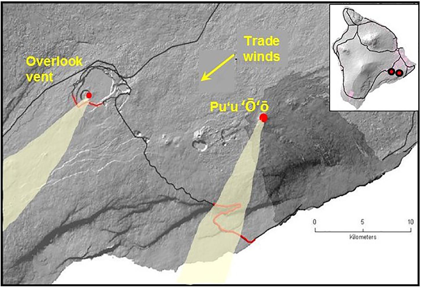
Figure 1. Location of the main sources of SO2 gas release at the summit and East Rift Zone of Kīlauea Volcano from 2014 to 2017, with inset of vent locations on the Island of Hawai‘i. The traditional road traverses (red lines) are located downwind of the outgassing sources during the dominant trade wind conditions (arrow).
Under prevailing northeasterly trade wind conditions, traverse measurements were most easily performed on Crater Rim Drive, which often intersected the plume less than 500 m from the gas emission source. Since the onset of the summit eruption in 2008 (Wilson et al., 2008) very high SO2 emission rates have frequently been observed from the actively degassing lava lake within the Overlook crater. The proximity of the traverse to the emission source, combined with the high SO2 emission rates, leads to frequent, very high SO2 column densities overhead (>10,000 ppmm). When such high column densities are encountered, several assumptions commonly made when evaluating DOAS or correlation spectroscopy measurements of optically thin plumes become inaccurate, and specialized methods must be applied (Millan, 1980; Kern et al., 2012; Fickel and Delgado Granados, 2017). Traditional DOAS measurements assume that the optical depth of the measurement is relatively small, with only a fraction of the initial radiance absorbed, and that the measured radiation has taken a straight path through the volcanic plume (see section “Conventional DOAS Retrievals”). Optically thick plumes introduce complex light paths for ground-based radiance measurements, complicate radiative transfer, exacerbate wavelength-dependent attenuation of the UV signal, potentially lead to total absorption of incoming energy at certain wavelengths, and interfere with the fitting of calibration cell spectra to the collected atmospheric sample spectra.
Kīlauea’s topography poses an additional challenge in quantifying summit emissions. Combined with the fact that the volcanic gasses were emitted from a vent within a ∼100 m deep crater, the shield volcano’s gentle slopes and strong trade winds often lead to very low altitude plumes. In fact, it is common for the gas plume to extend all the way to ground level. This makes application of scanning instruments for high-time resolution SO2 emission rate monitoring difficult because instruments placed downwind are often surrounded by gas and therefore cannot properly determine the SO2 load. Low angle scanning, as is required with a grounded or low altitude plume, yields measurements that are subject to atmospheric effects that plague low-angle viewing geometries (see Galle et al., 2003, for details). Challenges in accurately identifying the plume height, distance, geometry or speed for a low level dynamic plume contribute to widely varying results, with minimal constraint for realistically assessing results.
Difficulties in applying standard measurement techniques, combined with the desire for high resolution SO2 emission rate measurements, lead the U.S. Geological Survey’s Hawaiian Volcano Observatory (HVO) in 2012 to install an array of ten FLYSPEC spectrometer systems at the summit of the volcano (Horton et al., 2006). These instruments are permanently installed at a fixed distance of ∼3 km from the Overlook Vent. They are in the predominant downwind direction and are separated laterally by 250–880 m (Figure 2). They each have a fixed, upward-looking view, with spatial information on the plume overhead derived from the array’s layout rather than changes in the instruments’ viewing geometry (as is the case for traverse or scanning measurements).
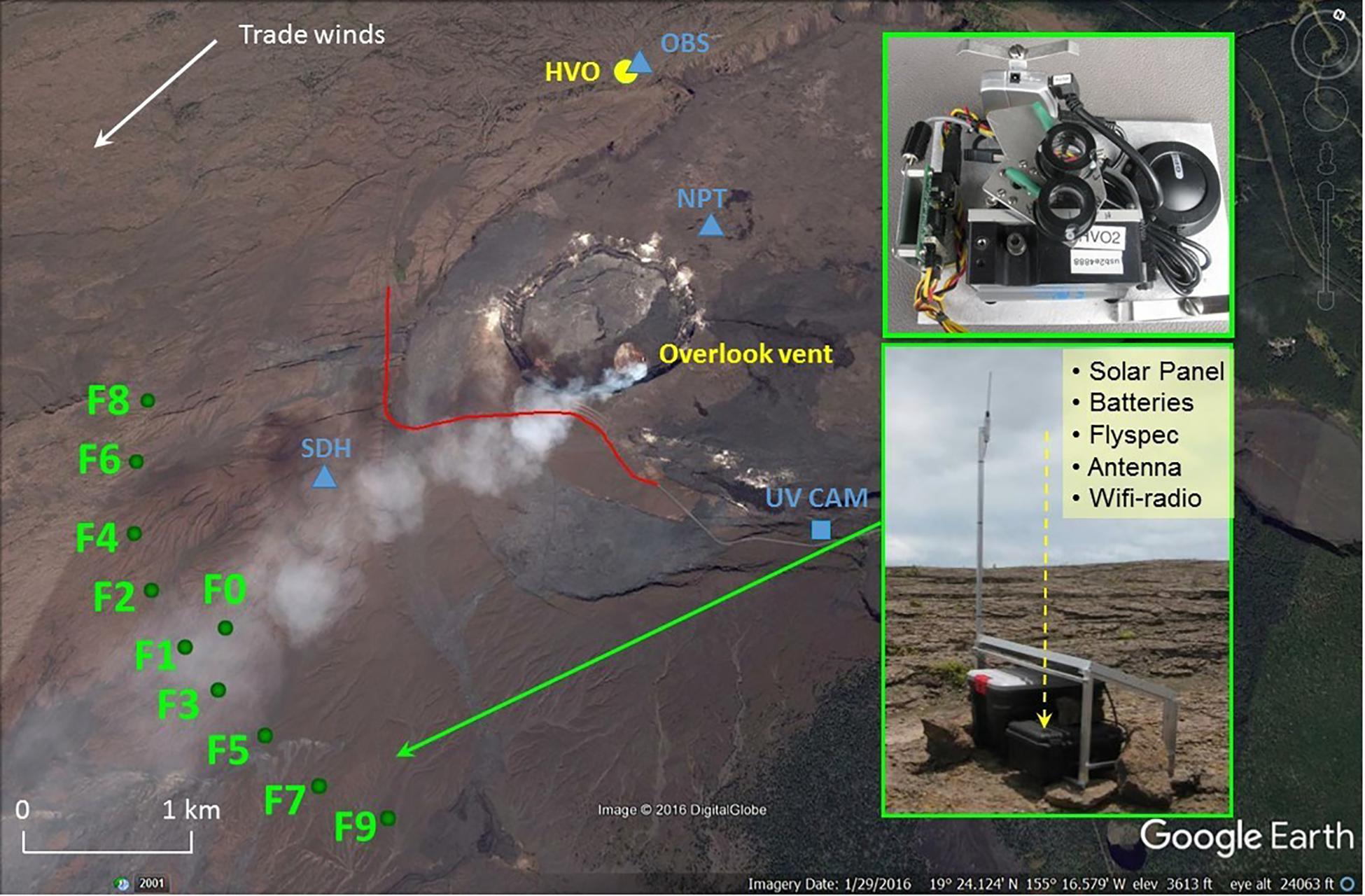
Figure 2. Location of 10-spectrometer upward looking FLYSPEC array downwind of the summit of Kīlauea (F0–F9), with station and instrument inset, ground-based anemometers and UV camera used for approximating plume speed (blue), traverse route on Crater Rim Drive (red), 2014–2017 location of Hawaiian Volcano Observatory and Overlook vent (yellow). Dominant trade wind direction indicated by arrow in upper left.
The advantage of the array-based data over scanning data is that the measurements are valid, even if the instruments are surrounded by volcanic gas due to a grounded plume. Also, the array’s 3 km distance from the vent makes for a more dilute plume than for road traverses on Crater Rim Drive thus allowing for quantification by DOAS or correlation methods. One disadvantage of the fixed array is degraded spatial resolution as compared to scanning or traverse techniques (see section “Errors Due to Location of Plume SO2 Maximum Between Array Sensors”). SO2 emission rates from Pu‘u ‘Ō‘o and other East Rift Zone (ERZ) degassing sources are still determined by vehicle traverses on Chain of Craters Road. As this road is 9 km from the gas source, plumes are generally quite dilute at the point of measurement and can therefore be accurately measured with standard DOAS or correlation analyses.
Focusing mainly on Kīlauea’s summit area in this study, we examine the SO2 emission rates determined by the FLYSPEC array from 2014 to 2017. First, we review the novel and conventional instruments and methods applied in this study and discuss the major sources of error and uncertainty. Next, we present our estimate of SO2 emission rates from the Overlook vent, along with the uncertainty in these results. To address the total SO2 degassing budget for Kīlauea Volcano, ERZ SO2 traverse measurements are also presented for the studied time interval. Finally, we compare our summit results to independent measurements using mobile and space-based platforms.
Instrumentation and Methods
Spectrometer Array
The FLYSPEC array is located about 3 km southwest of the active summit vent, and it extends along an arc about 3 km wide (Figure 2). Each instrument incorporates an Ocean Optics USB 2000+ spectrometer fitted with a 74-DA collimating lens (providing a field of view of 2.5°), a low and high concentration SO2 cell controlled by a servo motor, a GPS, and a netbook computer that controls the measurements (Businger et al., 2015). Column densities are retrieved on-site at each station. As is standard procedure for FLYSPEC instruments, the column amounts are retrieved by fitting the atmospheric sample spectrum to the gas cell calibration spectrum over the wavelength measurement window using the Levenberg-Marquardt least-squares fit. This compares the SO2 optical depth of the overhead plume with that of a known column density in the reference cells (Moré, 1978; Elias et al., 2006; Horton et al., 2006).
The calculated column densities are telemetered to HVO at a data rate of 1 Hz; the raw spectra are also stored should they be needed for future analysis.
Each station calculates the overhead SO2 column density at 1 s intervals between 0830 and 1700 Hawaii Standard Time when there is sufficient UV energy to obtain a reasonable signal-to-noise-ratio year-round in Hawai‘i. The SO2 load (X) in the plume cross section is then determined by summing the vertical column densities measured by the individual stations (i), according to equation 1:
where Si is the SO2 column density measured at station i and Δxi is the average distance between station i and the two adjacent stations. Most stations are located ∼300–400 m apart to capture the main features of the plume, which is typically between 1200 and 2800 meters wide and detected by 3–10 stations at any one time. Emission rates are then calculated from the SO2 load (X) in the plume cross section by multiplication with the wind speed (Horton et al., 2012; Businger et al., 2015).
The array’s distance from the vent means that the plume is significantly more dilute than when measured by road traverse on Crater Rim Drive. This reduces the complexity of the DOAS retrieval since the plumes are less opaque when crossing the array than when passing over Crater Rim Drive. However, overhead column densities more than 5,000 ppmm are still common. Therefore, spectral analysis is performed using a dual fit window (DFW) approach (see section “The FLYSPEC Dual Fit Window” and Horton et al., 2012; Businger et al., 2015).
Under prevailing trade wind conditions, the array generally spans the width of the plume, however, the processed emission rates must meet specific criteria for a measurement to be reported as valid. To assure that the plume is predominantly inside the array arc, a minimum of seven spectrometers in the arc must report valid column amounts, and the spectrometer at either end of the arc must report < 350 ppmm. These conditions consider the spatial resolution of plume features, and the diurnal influence on signal-to-noise. If these conditions are met, the plume direction is reported as the azimuth from the Overlook vent to the FLYSPEC station reporting the maximum overhead SO2 column density. A cosine correction is then applied to account for non-perpendicular plume direction over individual array segments.
Seasonal interruptions in the trade wind flow occur each winter and less valid data is available from the array.
Mobile UV Spectrometer Instruments
In this study, two types of mobile instruments were used to collect moderate resolution spectra of incident scattered solar UV radiation. For one, we used a mobile DOAS instrument consisting of an Ocean Optics spectrometer (either USB2000+ or SD2000) connected to an upward-looking telescope with a fused silica fiber optic cable. The spectrometers had an optical resolution of about 0.7 nm and recorded radiance in the 280–420 nm wavelength interval. For traverse measurements, the telescope was mounted on the outside of the vehicle (either car or helicopter), while the rest of the instrumentation was placed inside. A laptop computer acquired spectra with the Mobile DOAS software (e.g., Galle et al., 2003). The other instrument was the standard mobile version of the FLYSPEC described in section “Spectrometer Array” and by Horton et al. (2006).
Calculating SO2 Column Densities From UV-Spectral Data
Conventional DOAS Retrievals
The DOAS technique measures absorption of scattered solar radiation as it passes through a volcanic plume. Different trace gasses within the plume, and particularly SO2, have characteristic absorption cross-sections. This allows the selective detection of individual plume components. In conventional DOAS retrievals, quantitative measurements of column densities S are performed by comparing the spectrum of incident radiation obtained from the clear sky (I0) to that obtained from the volcanic plume (I). The column density, or number of gas molecules per unit area (c) along the effective line of sight of the instrument (L), can then be obtained by inserting the measured spectra into the Beer-Lambert-Bouguer law of absorption.
As the spectral optical depth τ and the absorption cross-sections σi are both vectors, the column density is obtained by fitting the absorption cross-sections of various trace gasses suspected in the plume to the measured optical depth. This approach has been shown to yield accurate trace gas column densities along the instrument line-of-sight if (1) the optical depth is relatively small so that only a fraction of the initial radiance is absorbed, and (2) the measured radiation has taken a straight path through the area of interest, in this case the volcanic plume (Perner and Platt, 1979; Platt, 1994; Platt and Stutz, 2008).
Complications arise if either of these two conditions are not met. If radiation is scattered within the volcanic plume, e.g., on aerosols or water droplets, then the effective light path along which the measurement is made may change. Though column densities S can still be retrieved in this situation, these can no longer be easily converted to average concentrations (Eq. 2) or cross-sectional plume loads if the effective path length L is unknown. Similarly, if a gas species in the plume absorbs more than a few percent of the incident solar radiation, the effective light path along which the measurement occurs begins to vary with wavelength, becoming shorter for wavelengths at which strong absorption occurs. This can lead to inaccurate column densities (several factors to orders of magnitude error) particularly when fitting uses the shorter wavelengths, where stronger absorption occurs (Mori et al., 2007; Kern et al., 2010, 2012; Fickel and Delgado Granados, 2017).
Several techniques have been suggested to avoid the problems associated with the complex radiative transfer effects (Mori et al., 2007; Kern et al., 2010, 2012; Fickel and Delgado Granados, 2017). The most straightforward method is to avoid measurements in conditions with very high SO2 column densities or high plume opacities (e.g., condensed plumes). This consideration was fundamental in determining the optimum location of the spectrometer array (Businger et al., 2015), which is close enough to capture short time-variations in the outgassed plume but avoids very high SO2 column densities.
When UV-spectroscopic measurements of optically dense plumes are evaluated with conventional DOAS approaches, the retrieved SO2 column densities have been found to depend on the wavelength range in which the spectral fitting is performed (Mori et al., 2007; Kern et al., 2010, 2012; Fickel and Delgado Granados, 2017). This is problematic, as the actual amount of SO2 in the instrument’s viewing direction should not depend on the wavelength of light that is being measured. Instead, this is an indication that the conventional DOAS model does not adequately describe the physical processes governing the scattering and absorption of UV radiation between the sun and the instrument. A more sophisticated model is needed.
Variable Wavelength Fit Windows
Conventional DOAS retrievals assume a linear relationship between optical depth and column density. This relationship breaks down for high optical depths if the spectrometer does not fully resolve the spectral absorption features, as is typically the case for miniature DOAS spectrometers and most target gas species. Fortunately, in the case of SO2, strong absorption can be avoided. Since the magnitude of the SO2 absorption cross-section decreases rapidly toward wavelengths longer than 300 nm, moving the range in which the spectral analysis is performed (i.e., the ‘fit window’) toward longer wavelengths decreases the considered optical depth of SO2 absorption.
Several algorithms have been suggested to take advantage of this circumstance. When analyzing data collected close to the fumaroles at Poas Volcano in Costa Rica, de Moor et al. (2016) dynamically adapted the lower end of their DOAS fit window to avoid SO2 optical depths greater than 0.1. In this study, we considered this same approach, which we call ‘Sliding Lower Fit Bound’ (SLFB), in comparison to other retrieval methods. The SLFB algorithm first performs a conventional DOAS SO2 retrieval in the 307 to 340 nm wavelength range. If the derived SO2 optical depth exceeds 0.1 in this window, the lower bound of the fit range is increased by one tenth of the total width of the fit window (3.3 nm in this case), and the fit is performed again on this new window. This process is repeated until the fit returns an SO2 optical depth below 0.1, at which point the retrieved column density is saved as the final fit result. To ensure that the number of pixels included in the fit always remained adequate to distinguish between the absorption features of SO2 and ozone (O3), the lower fit bound was not allowed to exceed 319 nm. The few spectra that did not return an optical depth below 0.1 with the 319 nm lower bound were omitted from the analysis. The algorithm aims to avoid high optical depths associated with SO2 absorption while at the same time allowing for high sensitivity at times when low SO2 loads are present in the instrument’s field of view. Fickel and Delgado Granados (2017) used a similar approach and suggest using one of three partially overlapping fit windows, with the choice of window depending on the SO2 column density derived in each.
The FLYSPEC Dual Fit Window
FLYSPEC instruments operate much the same as any other DOAS instrument but instead of fitting an SO2 absorption cross-section taken from literature, each FLYSPEC records its own SO2 absorption cross-section. This is achieved by inserting calibration gas cells of known SO2 concentrations into the light path and recording the instrument response. To account for any first-order changes in instrument response while operating in a range of typical SO2 column densities, two gas cells with different SO2 concentrations are measured – one with about 400 ppmm (low cell) and one with around 1500 ppmm (high cell) (Horton et al., 2006).
The SO2 retrieval used for operational analysis of FLYSPEC array data since 2014 at HVO is then very similar to the variable wavelength windows described above. The FLYSPEC ‘Dual Fit Window’ (DFW) approach selects the evaluation wavelength range based on how the encountered SO2 optical depth compares to that obtained when measuring the FLYSPEC calibration cells. If the SO2 optical depth is less than that of the low cell, then a fit window of 305 to 315 nm is used, and the low cell provides the absorption cross section for the fit. If the SO2 optical depth is larger than that of the low cell (cellL), but smaller than that of the high cell (CellH), then two fits are performed in the 305–315 nm window, one using each of the cells as absorption SO2 cross section (Shigh and Slow), and the weighted mean of the two results is calculated:
Finally, if the SO2 optical depth is greater than that of the high cell, then a second fit window is added. The SO2 cross section from the high cell is now fit to the measured optical depth in both the 305–315 nm (short) fit window and in the 319.5–330 nm (long) fit window, resulting in two SO2 column densities, Sshort and Slong. If the long-fit window returns less than 1.5 times the SO2 optical depth of the high cell, then a weighted average is calculated between the two different fit results according to:
with
For SO2 column densities larger than 1.5 times that of the high cell, the result from the long-fit window is used exclusively, with the high cell acting as the SO2 reference cross section.
A logic diagram for selection of the FLYSPEC evaluation window is included in the Supplementary Material.
Simulated Radiative Transfer DOAS
To avoid strong SO2 absorption, column densities can be measured at greater downwind distances and/or the fit wavelength range can be adjusted. However, these strategies do not account for signal dilution caused by radiation entering the field of view between the plume and the instrument or in-plume scattering on aerosols or condensed water droplets (Kern et al., 2010). At Kīlauea’s summit, signal dilution is likely a minor concern since the plume is typically within 10’s of meters of the ground, and all the measurements we are reporting were performed in a zenith-looking geometry. In-plume scattering, however, could cause inaccuracies in SO2 retrievals, particularly when the measured plume is visibly opaque. An approach called Simulated Radiative Transfer DOAS (SRT-DOAS) was developed to deal with realistic radiative transfer in volcanic plumes (Kern et al., 2012) and applied to dense plumes detected at Kīlauea’s summit in 2010–2011. This method uses a three-dimensional radiative transfer model to simulate the propagation of light in and around an idealized volcanic plume and compares the modeled spectra with measured ones. The best match between measurement and model yields the plume properties, such as the SO2 column density.
Simulated Radiative Transfer DOAS can account for complex light paths in and around volcanic plumes, but also has drawbacks when compared to the previously mentioned methods. SRT-DOAS retrievals rely on the availability of a lookup table of modeled spectra, which are computed by considering all possible measurement conditions in a radiative transfer model. This is a computationally expensive and time-consuming task. Typically, the plume geometry and atmospheric conditions are kept constant, while the plume SO2 loading and aerosol optical depth are varied to reflect all possible combinations of these parameters. The method is therefore limited to situations in which the plume geometry and atmospheric conditions are reasonably well constrained and constant during the measurement interval. Errors in the initialization of these parameters can cause systematic errors in the results. For these reasons, the method is currently not used for routine analysis of DOAS data, but rather only used in case studies where these external parameters can be adequately constrained.
Long UV Wavelength SO2 Fit Window
Bobrowski et al. (2010) documented the use of a wavelength range at the long end of the UV spectrum (360–390 nm) specifically for examining plumes with high optical depths. We utilize this window for evaluating the very large column densities encountered during road traverses conducted along Crater Rim Drive (section “Spectrometer Array”). This wavelength window makes use of SO2 absorption lines stemming from the spin-forbidden a3B2 ←X1A1 transition of the SO2 molecule which are about two orders of magnitude weaker than the lines in the standard DOAS 310–325 nm wavelength region. Therefore, this retrieval window is insensitive to low SO2 column densities but avoids strong SO2 absorption and is therefore less affected by radiative transfer complexities in cases where extremely high SO2 column densities (e.g., >10,000 ppmm) are encountered.
Determining Plume Speed
Regardless of the type of spectroscopic retrieval method, the plume speed is required to derive emission rates from cross-sectional SO2 loads. In this study, three different methods were employed to determine plume speed based on the location of data collection.
Cross-Correlation Method
The spectrometer array was designed to allow continuous monitoring during daylight hours of SO2 emission rates from the Overlook vent. To determine wind speed, a single spectrometer station was positioned 100 m closer to the vent than the rest of the array in the predominant trade wind direction (F0 in Figure 2). Overhead SO2 column densities recorded every 10 s by this station are used to determine plume speed using a cross-correlation approach (Williams-Jones et al., 2006). A 10-min time series of SO2 column density is generated every minute and is compared to the 10-min time series recorded by station F1, 100 m downwind. Examining the time lag between the two stations, the maximum cross-correlation between the time series is sought, which is representative of the time it takes for plume features to pass from station F0 to F1. The plume speed can therefore be determined by dividing the 100-m distance by the derived time lag.
Next, a quality filter is applied to the derived plume speeds to ensure that only valid data are reported. The plume speed is deemed valid if (1) the peak of the plume is recorded within the central part of the array (stations F1–F7), (2) stations F0 and F1 recorded column densities above the detection limit during at least 3 of the last 10 min and, (3) the calculated plume speed is less than twice that measured by a nearby anemometer (SDH Station, see next section). If any of these conditions are not met, the nearby anemometer wind speed is used to determine the emission rate.
Anemometers
When volcanic gas is passively released into the atmosphere, it quickly mixes with background air and travels together with surrounding air parcels. Therefore, wind speed can be an appropriate measure for plume speed in these situations. Although it is not usually possible to measure wind speed at the precise location of the plume using conventional methods, anemometers near ground level can provide useful information, particularly during times when other wind data are not available, or the plume is grounded. Gill ‘Windsonic’ ultrasonic anemometers are located 3 m above ground level (agl) ∼0.8 km north of the Overlook vent (station NPT) and the FLYSPEC array (station SDH). RM Young propeller and vane style anemometers are located 10 m agl on the north side of HVO on the rim of Kīlauea Caldera (station OBS, Figure 2). Measurements from these instruments are compared with other methods for determining the wind speed.
Plume Speed From SO2 Camera Imagery
Time-resolved imagery of volcanic plumes can also be used to derive plume speeds. During the period of this study, HVO maintained an SO2 camera on the southeast rim of Kīlauea Caldera (Kern et al., 2015). Aimed at the Overlook vent, this camera records UV images of the plume at two 10 nm-wide wavelength channels centered at 313 and 330 nm. Images are recorded every few seconds, with repeat intervals depending mostly on telemetry network latency. These images are used to derive SO2 optical depths and, in combination with plume speeds measured by an optical flow algorithm, determine the SO2 emission rate at high time resolution (e.g., Mori et al., 2006; Bluth et al., 2007).
Several studies have examined potential error sources in wind speed determination using optical flow models (Peters et al., 2015; Klein et al., 2017; Gliß et al., 2018). Thus, for the case studies presented here, plume features in the SO2 camera imagery were manually tracked to calculate plume speed. A sequence of images was loaded for each period in question. In each sequence, prominent plume features were identified, and their movement was tracked through the sequence. The horizontal pixel displacement was calculated by simple differencing of subsequent feature pixel positions, and the pixel velocity was determined by dividing the displacement by the time difference of the respective images. The pixel velocity was then converted to an apparent plume speed (perpendicular to the camera’s viewing angle) by multiplying the pixel velocity and pixel size at the distance to the plume (approximately 0.75 m, see Kern et al., 2015 for details).
In a final step, the derived plume speed was adjusted to account for potentially non-perpendicular viewing geometry. Each instance in which the SO2 camera imagery was used to determined plume speed corresponds to a coincident vehicle traverse performed on Crater Rim Drive. The wind direction was determined by fitting a Gaussian curve to the progression of SO2 column densities measured while traversing the plume, then calculating the direction from the vent to the peak of this curve. Multiplication of the camera-derived plume speed with the sine of the wind direction minus the camera viewing direction yielded the corrected plume speed.
Given that this is a direct observation of the plume propagation, this method is deemed to be accurate for determining plume speed above the Overlook vent. However, various parts of the plume move at slightly different speeds. Therefore, the procedure was repeated 4 times for every measurement period, and the mean and standard deviation of each value are reported below.
The SO2 camera relies on imagery taken in only 2 wavelength channels (on SO2 band at 313 nm and off SO2 band at 330 nm) to derive the SO2 column density of the plume. Recent findings suggest that this limited spectral information is not sufficient to obtain an unambiguous calibration in cases where plumes with high SO2 loading and aerosol optical depth are encountered (Kern et al., 2013). In such situations, a collocated DOAS spectrometer can provide image calibration information, but this procedure relies on the same spectral retrieval methods used in our comparative study. Thus, a comparison of SO2 camera and array derived emission rates is not presented in this study.
Uncertainty and Error Sources for Spectrometer Array Derived SO2 Emission Rates
In the previous section, the methods used to evaluate data from the fixed spectrometer array were described. To quantify the uncertainty of our measurements, we now evaluate results using different fit-windows, plume speed data, and traverse measurement strategies.
The Impact of Fit Window
Several different spectral retrievals were introduced in section “Calculating SO2 Column Densities From UV-Spectral Data,” each representing a slightly different method for determining SO2 column density along the instrument line of sight from the measured UV-spectral data. To test the sensitivity of the array measurements to different spectral retrieval methods, we performed a targeted experiment. On May 24, 2017, a mobile DOAS instrument was collocated with the F0 spectrometer array station. The DOAS telescope was mounted vertically on the FLYSPEC antennae mast, pointing toward zenith. Spectra were recorded from this stationary location at 1 s intervals between 12:49 and 14:46 local time.
The mobile DOAS data collection output format lends itself to performing a variety of spectral analyses using existing processing routines. Thus, we performed SO2 column density retrievals on the collected (stationary) mobile DOAS data using four different analysis methods. The evaluation parameters for each method are summarized in Table 1 (also see section “Calculating SO2 Column Densities From UV-Spectral Data”). We ran conventional DOAS retrievals in two fixed-fit windows, as well as a very long wavelength range specific for high column densities (Bobrowski et al., 2010). Conventional DOAS retrievals used the 310–325 nm window, which is the standard range used for analyzing scanning DOAS data in the ‘Network for Observation of Volcanic and Atmospheric Change’ (NOVAC) network (Galle et al., 2010). For comparison, we added a 319–340 nm fixed window evaluation which is more suitable for the large SO2 column densities encountered at Kīlauea’s Overlook vent. This longer wavelength window has a lower sensitivity to SO2, as it omits some of the strongest SO2 absorption lines. Therefore, the retrieval will have a reduced signal-to-noise ratio for low SO2 column densities. The use of a SLFB window mitigates this effect, and we ran an SLFB retrieval in which the lower fit bound varied between 307 and 319 nm (see section “Variable Wavelength Fit Windows”). An additional very long wavelength window (360–390 nm) was used for evaluating data collected during vehicle traverse measurements on Crater Rim Drive, where column amounts often exceeded 2,500 ppmm. A fourth and final analysis of the spectra was performed using an SRT-DOAS retrieval initialized with the approximate geometry of the measurements (see Table 1).
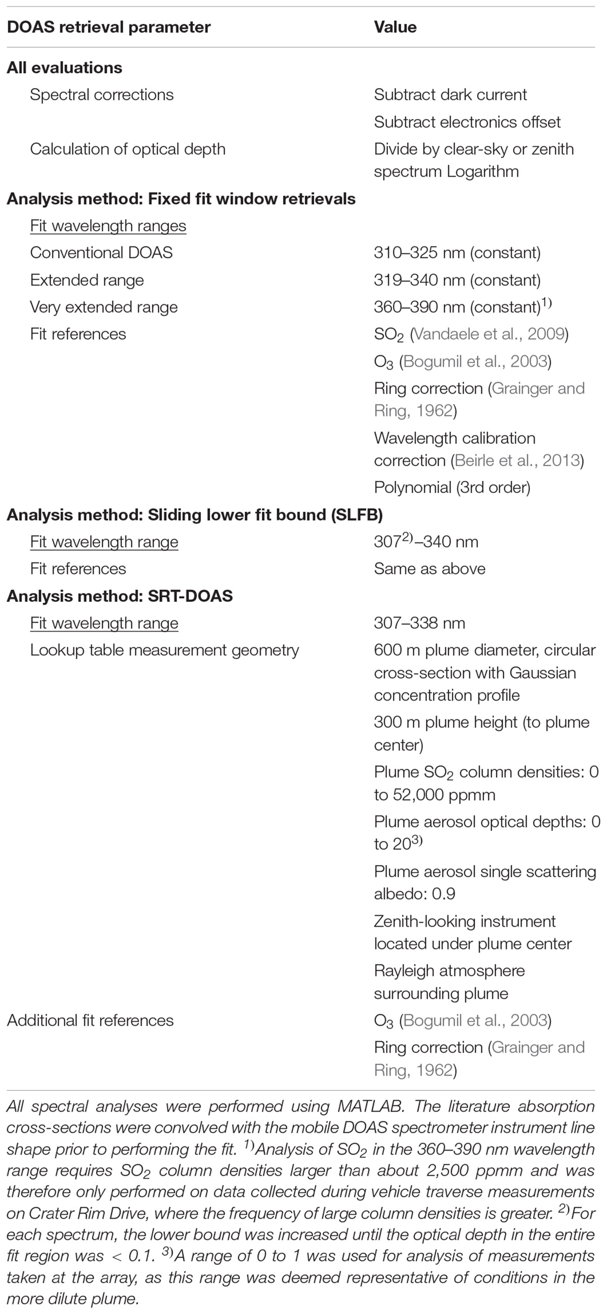
Table 1. Parameters defining SO2 retrievals compared in this study.
Figure 3 shows results of each spectral analysis method plotted against results obtained from a coincident measurement of FLYSPEC station F0 evaluated with the DFW technique. The main sources of scatter in the data are (1) lack of time synchronization between the upward-looking stationary mobile DOAS and array station F0 (the available FLYSPEC data were stored as 10 s averages, then interpolated to the 1 s measurement interval of the mobile DOAS) and (2) a slight mismatch between the viewing directions and viewing angles of the two instruments. The discrete steps in the SRT results are artifacts caused by the limited resolution of the lookup table.
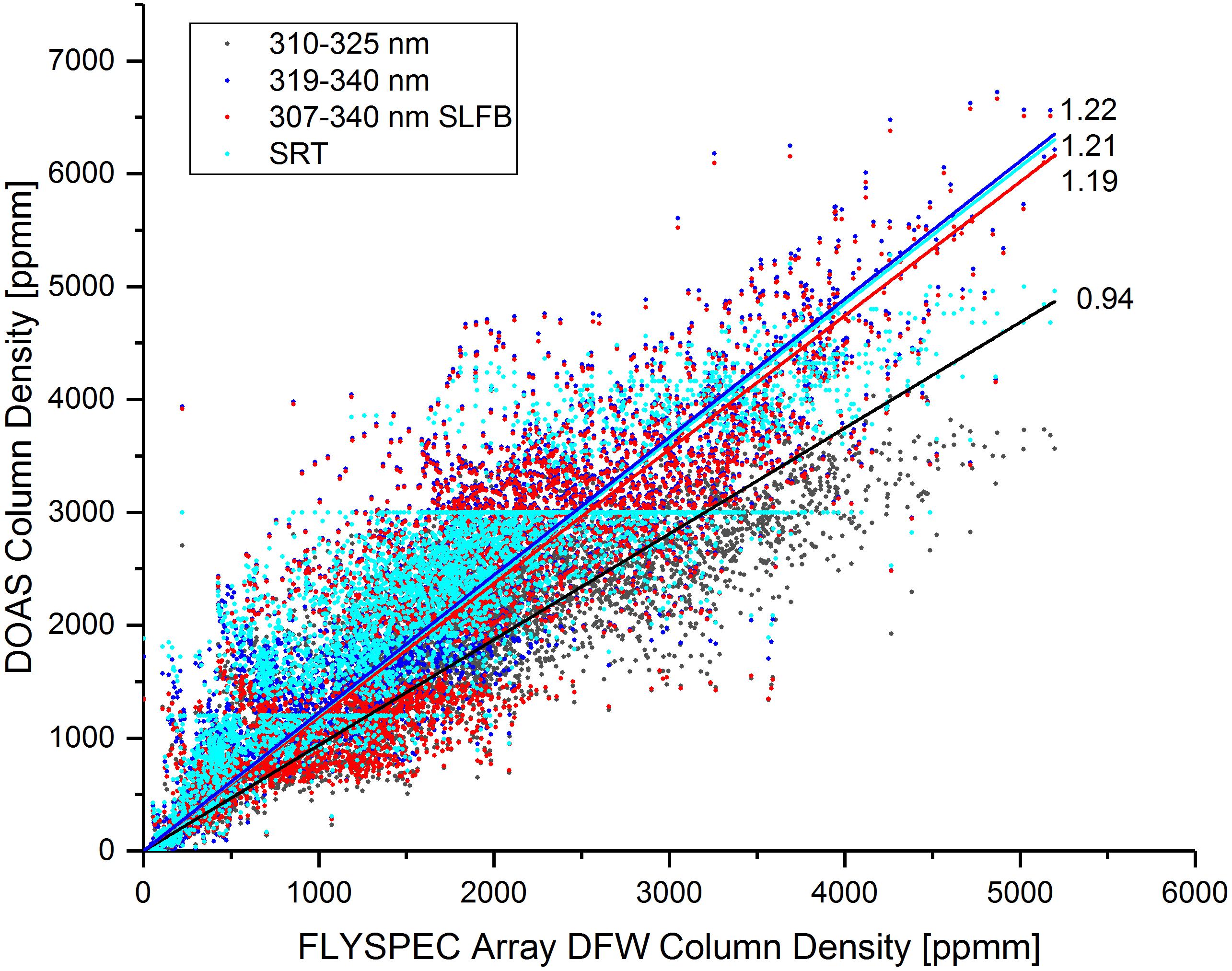
Figure 3. Coincident measurements of FLYSPEC station F0 and co-located stationary upward looking DOAS instrument are analyzed to compare the FLYSPEC DFW spectral analysis method with four different DOAS retrievals. Linear regressions were fit to the results of each method and show systematic differences are relatively small. A conventional DOAS analysis in the 310–325 nm window yields 6% lower values than the FLYSPEC DFW, while the results of the other methods are between 19 and 22% higher than the DFW.
Despite the scatter, linear regressions to each dataset reveal slight systematic differences between the analysis methods. Conventional DOAS retrieval in the 310–325 nm wavelength window systematically yields 6% lower SO2 column densities than the DFW method. All other methods return values slightly higher than the DFW method, with the 319–340 nm DOAS retrieval giving 22% higher values, the SLFB retrieval giving 19% higher values, and the SRT-DOAS retrieval giving 21% higher values on average.
The systematic difference between the methods is not unexpected. The presence of aerosols in the plume overhead causes a non-negligible contribution of complex light paths to the radiance measured by the instruments on the ground. Since, in this situation, the path of light through the plume will depend to some degree on its wavelength, the various retrievals will give different results based on which wavelengths are used.
Retrievals using a broad fit window are dominated by the shorter, strong absorption wavelengths. Thus, the SLFB retrievals are nearly identical to the traditional DOAS fit window when measuring low column amounts, even though the SLFB includes wavelengths out to 340 nm. As column amounts increase, the sliding fit window and DFW do a better job quantifying column amounts than would a single broad fit window.
The SRT-DOAS method uses the wavelength-dependency of the fit results to derive information on the radiative transfer of the measurement, but it requires additional assumptions on the conditions within and around the plume. For example, we consider the plume to be 600 m wide with a circular cross-section and a Gaussian concentration profile. Clearly this is an idealized scenario, and actual conditions will vary, potentially skewing the results. Therefore, an agreement of all methods within 22% of the DFW method is considered a successful validation of this method, and we consider other sources of uncertainty in the emission rate calculation (e.g., wind speed) are likely of similar or larger magnitude.
Based on these results, we consider the 1-sigma uncertainty of the SO2 column density DFW results to be about 22%.
The Impact of Plume Speed Source on Calculated Array Emission Rates
Obtaining an accurate plume speed is addressed by using several methods for the summit vehicle traverse and array-based emission rate measurements. When plume geometry does not allow array-based plume speed calculations using the cross-correlation technique, wind data collected 3 m agl, approximately 800 meters from the array mid-point (SDH station; Figure 2) are used to derive array emission rates.
A plot of ground-based (SDH anemometer) wind speed, and array-based (cross-correlation) plume speed for the time interval of June – September 2017 yields a linear regression with a 22% difference for the two methods during representative trade wind conditions (Figure 4). The error in the SDH ultrasonic anemometer wind speeds is reported by the manufacturer as ± 2% at 12 m/s, while the total uncertainty in the cross-correlation plume speed determination for instruments separated by 100 m is < 5% (Williams-Jones). For our configuration and conditions, this error is expected to be larger due to imperfectly synchronized computer clocks, indirect plume travel from array station 0 to 1, and imperfect plume feature correlation by the automated algorithm.
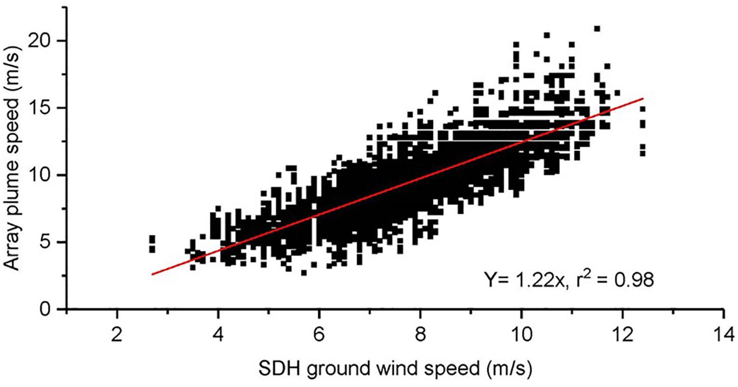
Figure 4. Plume speed calculated from peak correlation using two along-axis FLYSPEC instruments versus 3-m agl wind speed measured with an ultrasonic anemometer (station SDH; Figure 2) for June–September 2017. Data is filtered to include only plume speeds used to calculate emission rates (see section “Spectrometer Array”).
The difference between array plume speed and 3-m agl anemometer wind speed is not unexpected given likely variability of the vertical wind profile. Horizontal mean wind speeds measured by the SDH anemometer are affected by friction and surface roughness as air passes over the ground. Under moderate trade wind conditions, the top of the plume typically reached 500–800 m agl (Patrick et al., 2018); thus, plume speeds tracked by the array are expected to be somewhat larger, depending on the altitude of the plume.
Errors Due to Location of Plume SO2 Maximum Between Array Sensors
The track of the summit SO2 plume is quite predictable during typical trade wind conditions. Stations located toward the statistical center of the plume are spaced more closely together (250–400 m), while the stations most likely to be at the edges of the plume are spaced further apart (450–880 m). Strong winds result in a narrow plume, and the plume’s core can fall between adjacent sensors, particularly when the plume is located toward the edges of the array where instrument spacing is greater. In these instances, the peak of the plume can go undetected and the shape of the plume is inaccurately captured, resulting in an underestimation of the emission rate. The effects of this issue can be seen in the comparison of the helicopter traverse and array data (see section “Validation of Array Emission Rates Using Other Measurement Strategies”). We estimate that under-reporting of emission rate is most likely to occur during wind directions between 0 and 20° and >50°, which occurred ∼15% of the time for our data set. Based on our case study, we estimate the magnitude of the under-reporting of the emission rate is on the order of 30–50% for data collected during periods when the plume maximum falls between the sensors, but this will vary depending on the location and width of the plume.
Results
SO2 Emissions From Kīlauea Volcano 2014–2017
The SO2 budget for Kīlauea during this period includes emissions from both the summit Overlook vent and the ERZ (primarily the Pu‘u ‘Ō‘o vent). While SO2 release from the ERZ was dominant from 1983 until the opening of the Overlook vent in 2008 (Elias and Sutton, 2017), summit emissions were an order of magnitude greater than those released from the rift during 2014–2017. For historical context, the road-based SO2 emissions collected downwind of the Pu‘u ‘Ō‘o vent are included here, although they represent less than 10% of the total Kīlauea emissions for the reported era. The ERZ SO2 values were all measured using an upward looking mobile FLYSPEC ∼10 km downwind of the gas emission source, where the plume is relatively weak and homogeneous, with column amounts generally < 500 ppmm. Thus, the complexities caused by very high plume optical depths are not a factor for ERZ measurements.
Long-Term SO2 Output
Figure 5 presents the 10-s, daily-, and monthly mean SO2 emission rates calculated using summit FLYSPEC array measurements. Averages are presented for days with at least 2 h of valid 10-s data, which reduces the likelihood of atypical conditions influencing the average. Emission rates averaged over a month used all valid 10-s values for the period. Emission rates calculated using SDH wind speeds (<10% of the data set) have been adjusted by +22% to account for the systematic underestimation of the ground-based wind measurements for plumes aloft (section “The Impact of Plume Speed Source on Calculated Array Emission Rates”). The uncertainties in the array values are based on the uncertainty in SO2 column amounts (∼22%), plume speeds (∼5–30%), and underestimation due to plume maxima occurring between sensors (30–40% -see section “Errors Due to Location of Plume SO2 Maximum Between Array Sensors”). These factors result in individual emission rate value uncertainties of ∼30–50%.
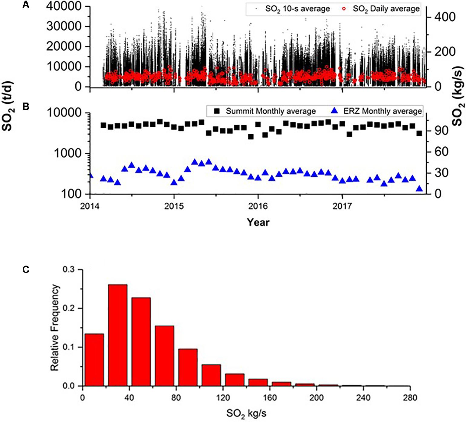
Figure 5. (A) SO2 10-s (black dots) and daily (red circles) average emission rate time series from Kīlauea Volcano summit array measurements 2014–2017. Daily means are reported for days with at least 2 h of data. For display purposes, infrequent values (<0.5% of data) above 40000 t/d are not shown. (B) Average SO2 release over a month (black square) was calculated using all valid 10-s values during the period. East Rift Zone average monthly SO2 (blue triangles) were measured by vehicle traverse of Chain of Craters Road downwind of the Pu‘u ‘Ō‘ō vent (Figure 2). (C) Frequency distribution of summit array 10-s emission rate values show that 99% of the values are less than 200 kg/s (∼17,000 t/d), with emission rates most commonly between 20 and 60 kg/s.
The average monthly Kīlauea East Rift Zone emission rates are included in Figure 5B. Although a minor contribution to total emissions, fluctuations in ERZ emissions are correlated with notable changes in the eruption during the period of interest (e.g., Global Volcanism Program, 2014). The emission rate data presented in this paper are given in Elias et al. (2018).
For 2014–2017, Kīlauea released an average of 5100 t/d, or 1.9 ± 0.1 Tg/yr. This is consistent with the space-based OMI SO2 inventory performed by Carn et al. (2017), which ranks Kīlauea as the second highest passively degassing SO2 producer (behind Ambrym) for the period 2005–2015. Kīlauea emissions represent 8% of the total SO2 released from the 91 persistently degassing volcanic sources consistently detected from space by OMI (Carn et al., 2017).
SO2 Short-Term Variability Reflects Lava Lake Dynamics
The short-term summit SO2 release is highly variable and depends on the spattering or non-spattering condition of the lava lake (Elias and Sutton, 2012; Nadeau et al., 2015; Patrick et al., 2016a,b, 2017, 2018). Stagnant lake conditions resulted in decreased SO2 release, while vigorous lake spattering was reflected in increased SO2 emissions The SO2 signature is consistent with lava lake fluctuations driven by cycles of activity at shallow depth, close to the lake surface. The high resolution SO2 FLYSPEC array measurements have helped confirm the types of seismicity that are associated with shallow outgassing processes, with seismic energy < 0.2 HZ most clearly correlated with the outgassing signature (Figure 6).
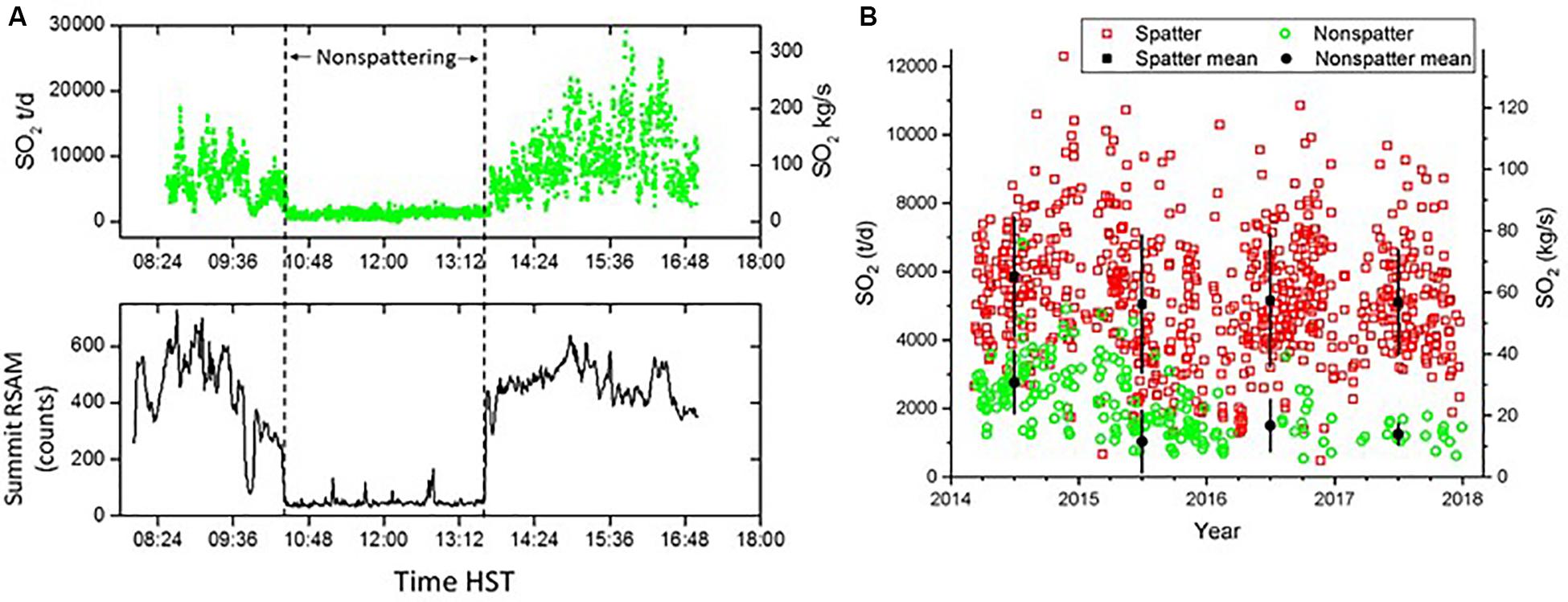
Figure 6. (A) SO2 emission rates (green) and relative seismic amplitude (RSAM, frequency > 0.2 Hz, black) during a transition between spattering and non-spattering lava lake conditions (marked by dashed lines) at Kīlauea Overlook vent on 9/9/2016. (B) Daily average SO2 emissions for lava lake spattering (red) and non-spattering (green) periods lasting > 1 h for 2014–2017. Non-spattering episodes are defined by RSAM level <100 counts. Annual mean and standard deviation are shown by black symbols for spattering (square) and non-spattering (circle) episodes. The sparser data at the beginning of each year reflects the seasonal nature of the trade winds. A lack of trade winds during the winter months results in fewer measurable plume configurations.
A record of SO2 emissions separated into spattering and non-spattering lava lake conditions is presented in Figure 6, and shows that on an annual basis, non-spattering lava lake phases correspond to SO2 emission rates that are on average 20–50% of those during spattering phases. This is consistent with findings of Patrick et al. (2016a,b). While the gas release during spattering phases was similar for 2014–2017, SO2 emissions associated with non-spattering intervals began to decrease in 2015, with a marked decrease in the occurrence of non-spattering events in 2016 (Patrick et al., 2018). This suggests changes in the permeability in the upper portions of the lava lake, possibly due to changes in circulation patterns, magma reservoir pressure, and/or magma supply rates. Oppenheimer et al. (2018) showed that the spattering regime releases larger gas bubbles, which may support the observation of more efficient decoupling of gas from the lake during spattering activity.
Validation of Array Emission Rates Using Other Measurement Strategies
Kīlauea has a long history of emission rate measurements (Elias et al., 1998; Elias and Sutton, 2002, 2007, 2012) and the spectrometer array represents the latest technological upgrade. Based on careful analysis of sources of error and comparison with other methods discussed in this paper, we consider emission rates recorded by the array as our best SO2 estimates for 2014–2017. However, since the array represents a new methodology for measuring emission rates at Kīlauea, the next section presents results of several experiments aimed at validation of this new technique.
Comparison of Array Emission Rates With Helicopter Traverses
We attempted to validate the array-based emission rates by traversing the plume using an upward looking DOAS mounted on a helicopter above the array, and ∼3 km further downwind. A range of plausible emission rates were calculated using the spectral retrieval methods as described in section “The Impact of Fit Window,” and the mobile DOAS reduction software. The array calculated plume speed was not available during the period of the helicopter traverses, therefore the wind speed from the 3 m agl SDH anemometer (location in Figure 2) was used. The traverse and array data were scaled up using the correction factor detailed in section “Long-Term SO2 Output.” A meteorological station located ∼5.5 km downwind of the vent (PKE) measures wind vector at 3 m agl (analogous to the SDH station) and showed that wind speeds near the location of the more distal traverses were less than 10% different than those measured by the SDH sensor near the location of the array.
For this case study, the DOAS helicopter traverse emission rates were higher, on average, than those reported by the array (Figure 7 and Table 2). Figure 7A presents the SO2 column amounts as measured by the helicopter traverse and reveals that the plume maximum fell between adjacent sensors F7 and F9 (odd numbered sensors are adjacent and span the east side of the array), and thus caused the array to miss the plume maximum and underestimate the total emission rate. The range of helicopter values represent minimum and maximum emission rates calculated using the 319–340 nm, SLFB, and DFW retrievals.
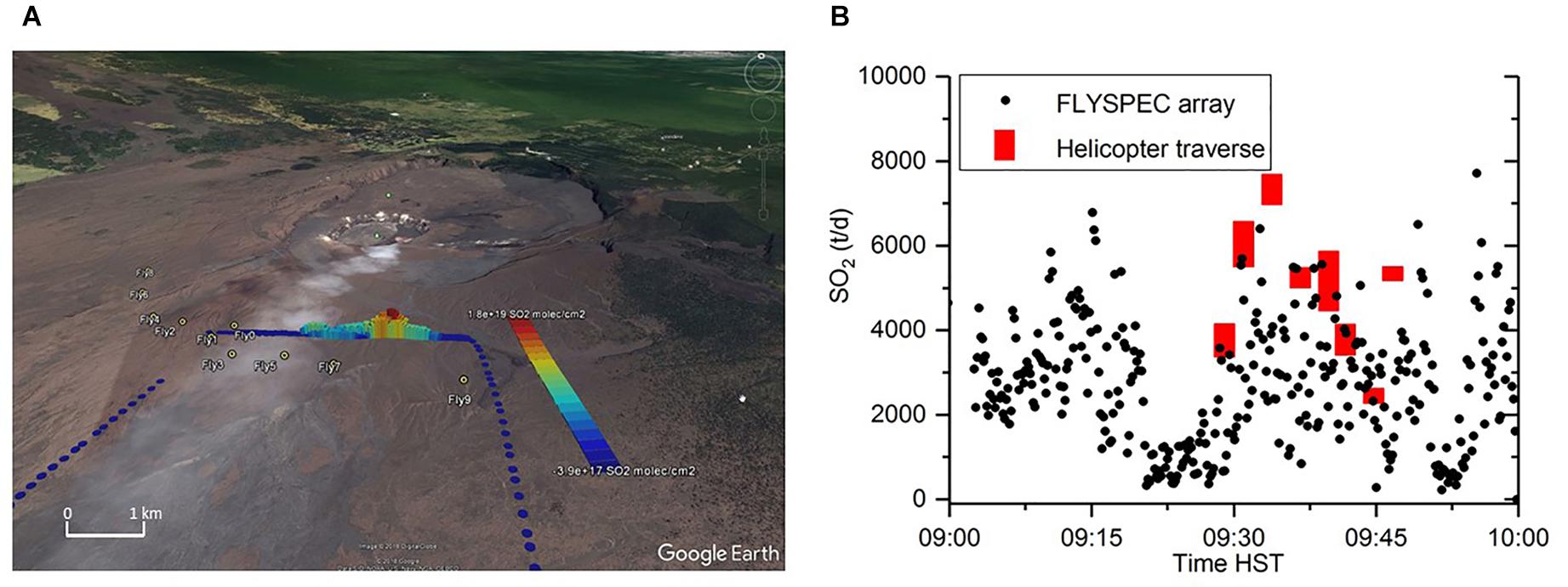
Figure 7. (A) SO2 column amounts during helicopter traverses measured with an upward-looking DOAS between 09:26 and 09:51 HST on 29 June 2017. The tracks are 3∼ km downwind of the vent and the warmer colors (yellow, orange, red) indicate higher SO2 column amounts. Note that the plume center is located between array stations F7 and F9, likely contributing to underestimated values by the array as compared to the helicopter traverse.Image ©2018 DigitalGlobe. ©2018 Google. (B) Time series of 10-s SO2 emission rates measured by the spectrometer array (black dots) between 09:00 and 10:00 HST on 29 June 2017. Red bars indicate the range of plausible SO2 emission rates derived from upward-looking DOAS traverses on a helicopter at the location of the array (first five measurements) and ∼3 km farther downwind (last 3 measurements) using the various spectral retrieval methods described in section “Calculating SO2 Column Densities From UV-Spectral Data.” The plotted times for the 3 downwind measurements were adjusted to account for plume travel time.
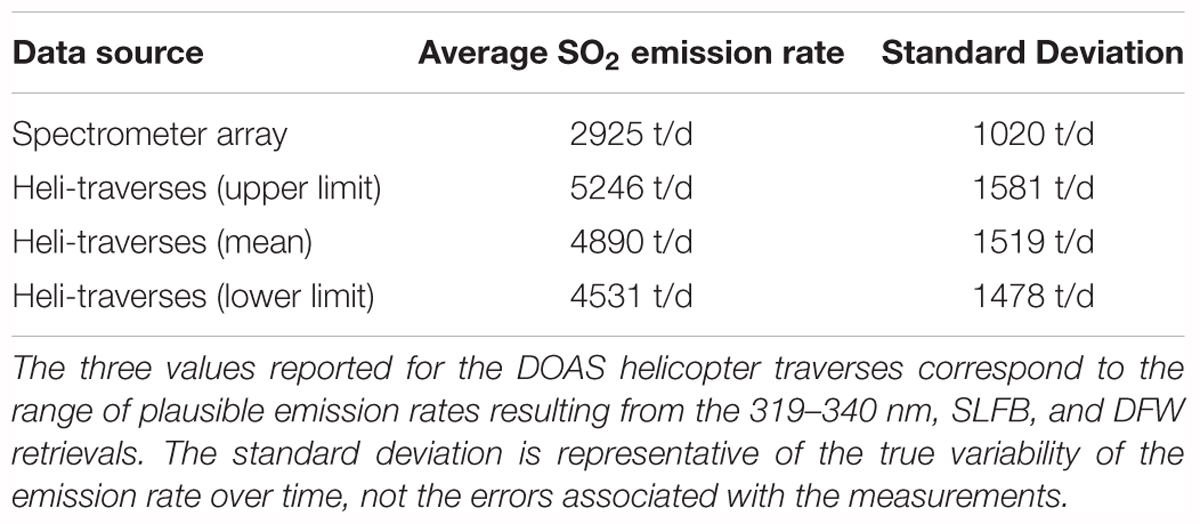
Table 2. Summary of average emission rates obtained from the array and by DOAS helicopter traverses above the array and 3 km downwind of the array between 09:29 and 09:53 Hawai‘i Standard Time (HST) on 29 June 2017.
This experiment exposes a potential weakness in characterizing an eruption plume using discrete sensors. While the column amount retrievals themselves agree well with other techniques, certain wind directions/plume positions will result in an underestimation of the emission rate. Some of the observed scatter in the array emission rates is likely due to this issue. However, averaged over time, the data provide a reasonable estimate of emission rates since prevailing trade winds generally blow the plume to the more densely instrumented center of the array. Helicopter measurements reduced using a retrieval algorithm equivalent to the array algorithm, return emission rates that significantly overlap the array 10-s values. The 2 techniques differ in measurement time-base, viewing geometry of the instruments, and measured plume transect. The dynamic nature of gas release and uncertainty in the maximum column amount position contribute to general agreement between the traverse and array data, rather than quantitative alignment. A single helicopter traverse performed at the array location on 3/30/2017 yielded an emission rate within 24% of the coincident array measurement.
Comparison of Array Emission Rates With Road Traverses
Before the establishment of the spectrometer array, HVO mainly relied on road-based FLYSPEC and DOAS traverses beneath the summit plume to assess the SO2 emission rate (Elias et al., 1998; Elias and Sutton, 2002, 2007, 2012). However, road traverses conducted on Crater Rim Drive have been challenging to interpret since 2008, with the onset of the current phase of activity at Kīlauea’s summit. Two significant factors, discussed below, are the retrieval of accurate column densities for the optically dense plume, and the measurement of an accurate plume speed. While the road-based data provide useful qualitative information on SO2 outgassing, they provide only general guidance on the quality of the array’s measurements.
Comparison of Different SO2 Retrievals for Road Traverses
At Kīlauea, Crater Rim Drive is the most accessible road that allows vehicle-based traverses to pass completely below the summit plume during the prevailing trade wind conditions. Its relative proximity to the location of the Overlook vent (<500 m) means that the overhead plume is more concentrated than at the location of the array further downwind. The much higher SO2 column densities and aerosol optical depths encountered on the road greatly increase the impact of radiative transfer in and around the plume. Therefore, conventional algorithms for retrieving SO2 column density may give inaccurate results (Kern et al., 2012) and careful treatment of the complexities of light scattering and attenuation is required.
To obtain an estimate of the uncertainty we may expect in SO2 column density measurements from Crater Rim Drive, we examined results of ten upward-looking Mobile DOAS traverses on 30 March 2017 using a variety of spectral analysis methods. In addition to applying all the DOAS retrievals used for comparison of the DFW technique at the location of the array (see section “The Impact of Fit Window” and Figure 3), we also analyzed the traverse data in the very extended wavelength fit window at 360–390 nm, as first suggested by Bobrowski et al. (2010) since SO2 column densities greater than 2,500 ppmm are frequently encountered (see section “Long UV Wavelength SO2 Fit Window”).
We also implemented a DFW retrieval analogous to that used to analyze the FLYSPEC array and applied this to the mobile DOAS spectra. Figure 8 shows how the results from various DOAS retrievals compare to those of the DFW method applied to the mobile DOAS data. Note that this plot encompasses column densities of up to 25,000 ppmm, a factor of 5 higher than the column densities measured at the location of the array. The road traverse column density comparison mirrors the general trend of the array column density comparison (section “The Impact of Fit Window”).
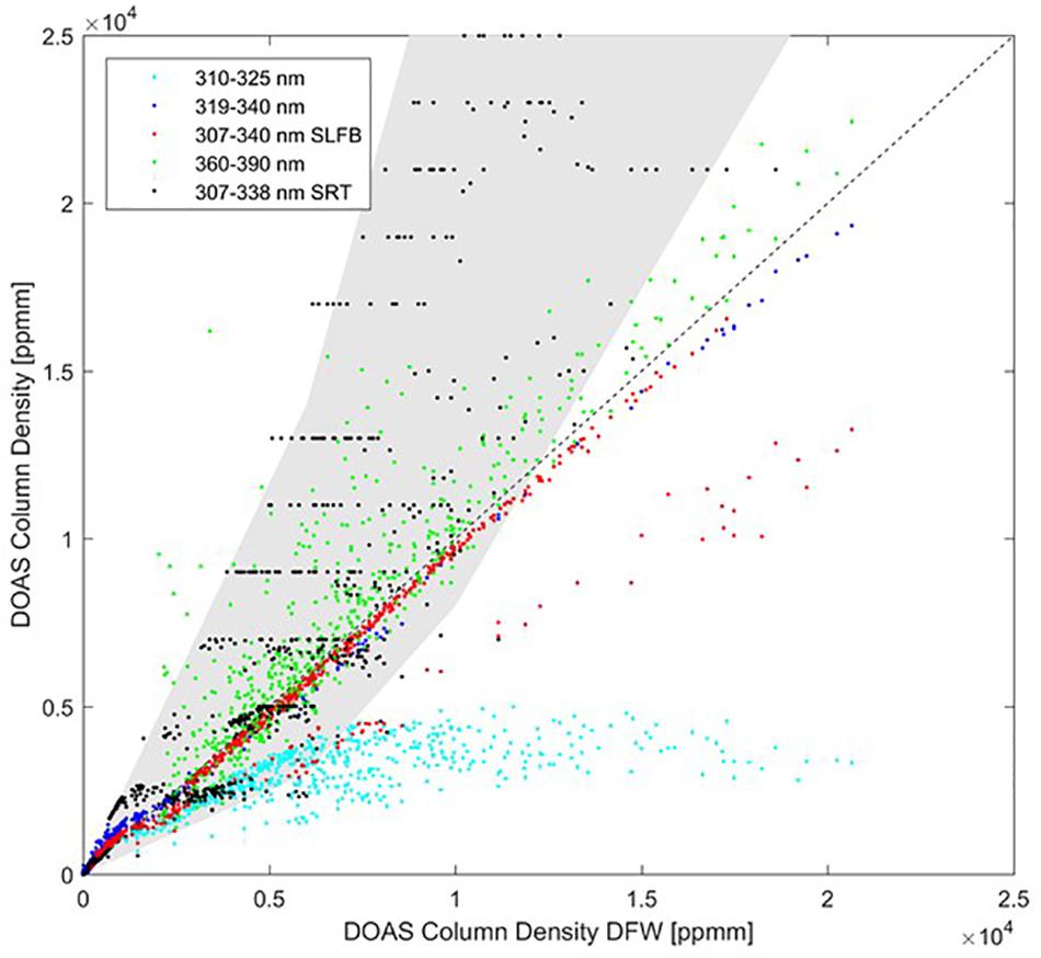
Figure 8. SO2 column densities obtained from ten road traverse measurements on Crater Rim Drive on 03 March 2017 between 10:50 and 11:55 HST. Column densities were evaluated with 6 different retrieval methods. In this plot, all column densities are plotted against the results obtained using a Dual Fit Window (DFW) approach that is equivalent to the spectral analysis procedure used to evaluate FLYSPEC mobile or upward looking array data.
As expected, the conventional DOAS analysis in the 310–325 nm wavelength range returns significantly lower SO2 column densities than all other methods once column amounts exceed around 1000 ppmm. The very strong absorption of SO2 in this wavelength range causes complex radiative transfer effects at higher column amounts (Kern et al., 2012), that are not well captured by this simple approach. Therefore, this retrieval method is not considered further in our comparison.
The 319–340 nm window, SLFB, and DFW all return similar results, though for very low column amounts the signal-to-noise of the 319–340 nm retrieval is inferior to that of the other two approaches. For column densities above 2,500 ppmm, the DOAS fit in the 360–390 nm wavelength region returns slightly higher (about 20%) SO2 columns than the DFW method, with more observed scatter.
Finally, the more complex SRT method returns a range of SO2 column densities (gray shaded region) that overlaps with the DFW results up to about 5,000 ppmm, but then returns column densities that are up to a factor of 2 higher. The horizontal spread in the SRT data apparent in the plot is caused by variability in the retrieved plume aerosol optical depth (AOD). In the SRT retrieval, an estimate of the AOD is derived together with the SO2 column density (Kern et al., 2012). In this case, however, the retrieval returned a relatively large uncertainty for the AOD, which causes a relatively large uncertainty for the SO2 column density (hence the wide range of reported values in the gray area). In the vertical direction, the discrete values for SO2 column density (i.e., horizontal lines) are artifacts that stem from the limited resolution of the SRT lookup table.
It is challenging to ascertain which of the applied retrievals generally yields the most accurate results overall, since each has advantages and disadvantages. The 319–340 nm, SLFB and DFW methods are all similar in that they include areas of the spectrum where the SO2 absorption is weaker than in the standard DOAS 310–325 nm window. In this manner, they avoid issues related to non-linear instrument sensitivity caused by strong SO2 absorption, but they do not account for potential changes of the effective light path in and around the volcanic plume due to scattering on aerosols, which as noted, can be significant. The SRT-DOAS retrieval does account for complex radiative transfer, but it relies on the accuracy of assumptions used to generate precomputed lookup tables which are then compared to the measurement spectra (see Table 1). For a limited case study such as presented here, these assumptions should be quite good, but short-term variability in atmospheric and plume conditions may still compromise the results. While SRT-DOAS provides insight into the potential magnitude of the errors, it is much more difficult to use this technique for routine monitoring.
Regardless of which method is most accurate in this scenario, the comparison shows that there is a much larger uncertainty associated with the column density retrieval for the large SO2 abundances encountered on Crater Rim Drive than for the more dilute plume at the location of the array, 3 km downwind (compare Figure 3). For the traverse case study, the retrieved column amounts from the various analysis methods range between about -30 to +100% of the DFW results as compared to -6 to +22% of the DFW results derived at the location of the array.
Comparison of Plume Speed Measurements for Analyzing Road Traverses
As discussed in section “Determining Plume Speed,” plume speed is a direct multiplier for deriving emission rate, and traditionally represents the largest overall uncertainty in SO2 flux measurements. HVO has several sources available for measuring plume speed in proximity to the Overlook vent. Plume speed can be taken from SO2 camera imagery, or the wind speed recorded by a ground-based anemometer can be used (section “Anemometers”).
To examine the uncertainty of our plume speed assumptions for the traverse measurements, we compared wind data from 3 days on which we have anemometer data, SO2 camera images, and coincident traverse measurements on Crater Rim Drive. On all 3 days, the traverse measurements were used to determine the wind direction, which then feeds into the determination of plume speed from the SO2 camera imagery. The wind speed comparisons for the individual days are shown in Figures 9A–C.
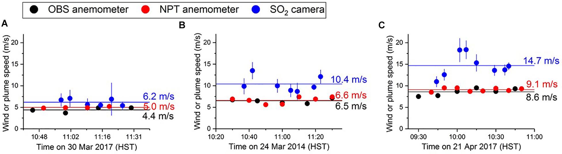
Figure 9. (A–C) Comparison of wind speeds derived from SO2 camera with wind speeds from meteorological stations OBS (10 m agl on rim of caldera) and NPT (3 m agl on floor of caldera; Figure 2) on three different days. Anemometer wind speeds are averaged over the intervals at which they are plotted. The SO2 camera wind speed was derived and plotted at times only coincident with DOAS vehicle traverse measurements performed on Crater Rim Drive.
On all 3 days, the average wind speeds obtained from the OBS and NPT anemometers were within 12% of one another, while the SO2 camera plume speed was systematically higher. The camera plume speeds also appear to be more variable than those reported by the anemometers; however, this is an artifact of different averaging methods for the anemometers (internal averaging over the 10–15-min interval) and the camera (discrete 10-s measurements averaged over the period of a single 3–5-min traverse.
The absolute difference between SO2 camera plume speed and anemometer wind speed appears to grow with increasing wind speeds. This is consistent with the expected vertical wind profile for plume speeds measured by the camera at 50–200 m agl. This discrepancy is expected to increase for larger wind speeds, and a power law is often used to describe the increasing horizontal mean wind speeds with altitude (also see section “Determining Plume Speed”). A reasonable agreement can be achieved between the anemometer and SO2 camera plume speeds by correcting the anemometer wind data, as is shown in Figure 10.
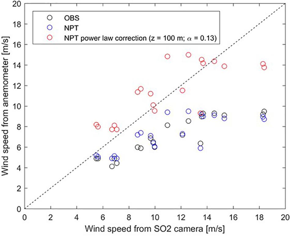
Figure 10. Comparison of wind speeds derived from the SO2 camera (horizontal axis) with wind speeds from anemometers at HVO and NPT. Data are from March 24, 2014, April 21, 2014, and March 30, 2017. Anemometer data is interpolated to timing of SO2 camera measurements. The wind speed calculated with SO2 camera data plot systematically higher than the anemometer data, with differences increasing for larger wind speeds. Applying a power law correction to the NPT data (red circles) brings them into the same range as the camera wind speeds.
Such a correction is extremely sensitive to the chosen model parameters (in this case the exponent), which depends on the surface roughness, a complex parameter and one that is especially difficult to estimate for the anemometer perched on the rim of the caldera. Applying a power law correction of the form v(z) = v(3m) ∗(z/3m)ˆα with z = 100m and α = 0.13 to the 3 m agl NPT wind speeds, brings them into the same range as the camera plume speeds, which were generally derived for a plume about 100 m above ground level. The α used here lies between values that characterize conditions over open water (0.11) and open land surfaces (0.143).
We also note that none of the measurement techniques, including the SO2 camera, measure plume speed at the exact location of Crater Rim Drive where the traverse measurements are made. Prior to 2008, gas emissions were characterized by a low ground-hugging plume which was predominantly influenced by wind speed. However, since the onset of the summit eruption, the plume buoyancy, rise rate, and horizontal speed are affected by both the local wind and lava lake conditions, which are extremely dynamic (Patrick et al., 2018). Therefore, it is not straightforward to correct the anemometer data to obtain accurate plume speeds for use in calculating emission rates from the road traverses. Instead, we interpret the discrepancy between our various methods of plume speed determination as an indicator of our measurement uncertainty. Based on the results obtained in the 3-day case study shown here, we expect that our wind measurements are within 30–40% of the true plume speed.
Comparison of Road Traverse and Array Emission Rates
We have shown that errors associated with obtaining accurate column densities and plume speed contribute to significant uncertainties in measuring SO2 emission rates by vehicle traverse on Crater Rim Drive under 2014–2017 degassing conditions. Here, we present examples of coincident traverse and array measurements to characterize the range of values that can arise with the noted uncertainties.
Figure 11 shows the time series of SO2 emission rates obtained from the spectrometer array (black dots) and by coincident mobile DOAS traverses (red bars) on Crater Rim Drive on March 30, 2017. The red bars indicate the range of values calculated for the DOAS traverses from the various SO2 spectral retrieval methods discussed in section “Comparison of Different SO2 Retrievals for Road Traverses.” The traverse measurements are shifted by +7 min to account for the time it took the plume to travel the 2.5 km from Crater Rim Drive to the array. The array values were calculated using the cross-correlation method for determining plume speed, and the traverses were analyzed assuming a plume speed of 4.4 m/s. This corresponds to the average wind speed measured by the OBS anemometer during the measurement interval, and based on the case study for this day, is assumed to be accurate within about 30–40%. The OBS station (Figure 2) wind speed value has historically been used to calculate road-based emission rates.
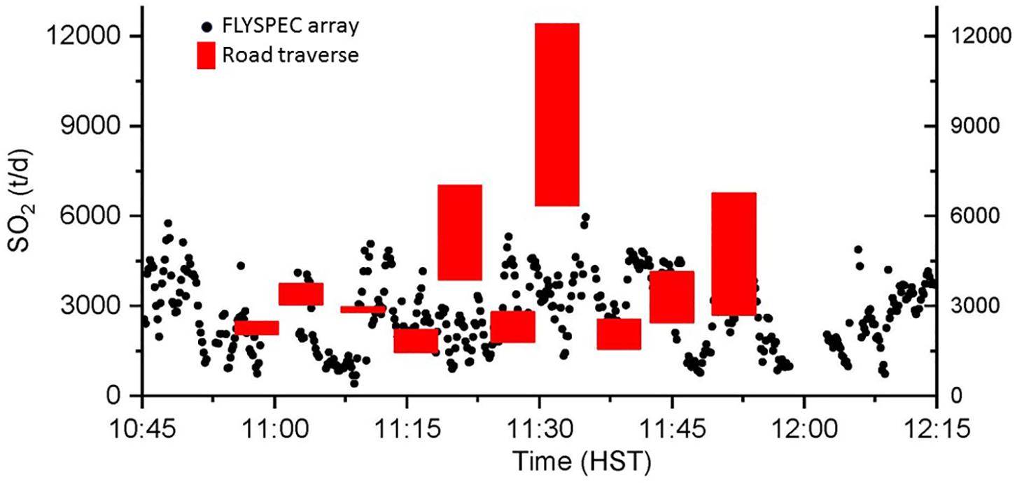
Figure 11. Comparison of SO2 emission rates from the FLYSPEC array (black dots) and the road- traverses (red bars) on March 30, 2017. The red bars indicate the range of values obtained from the various analysis methods described in section “Comparison of Different SO2 Retrievals for Road Traverses.” A constant wind speed of 4.4 m/s was assumed in analyzing the traverse data, which corresponds to the average wind speed measured by the OBS anemometer during the measurement period.
On the day presented here, the DOAS traverse and array emission rates agree broadly, with some notable outliers, which may be related to plume heterogeneities. As the plume emitted from the Overlook vent drifts downwind, it is mixed with background air by turbulent diffusion. This process reduces spatial gradients in SO2 concentration. Road traverses might pass directly under clouds of concentrated volcanic gas, then pass between such clouds in the next measurement. By the time the plume reaches the array, concentrated gas clouds are diluted, and gaps between such features have been at least partially filled in by gas from surrounding clouds. Therefore, the array will measure a more homogeneous plume. Road traverse results that are higher than array results may also be due to plume maxima falling between array sensors, yielding underestimation of emission rates by the array (see section “Errors Due to Location of Plume SO2 Maximum Between Array Sensors”).
The road traverse results on this day show atypical agreement with the array data (Figure 11 and Table 3). In general, the long-term road data record underestimates the emissions as compared to the array – on average, by about 60%. We attribute this to a combination of underestimated plume speeds and underreporting of column amounts due to radiative transfer issues. There may be a maximum threshold for the column amounts measured close to the vent, and thus, consistent under-reporting of emission rates calculated for Crater Rim Drive road traverses.
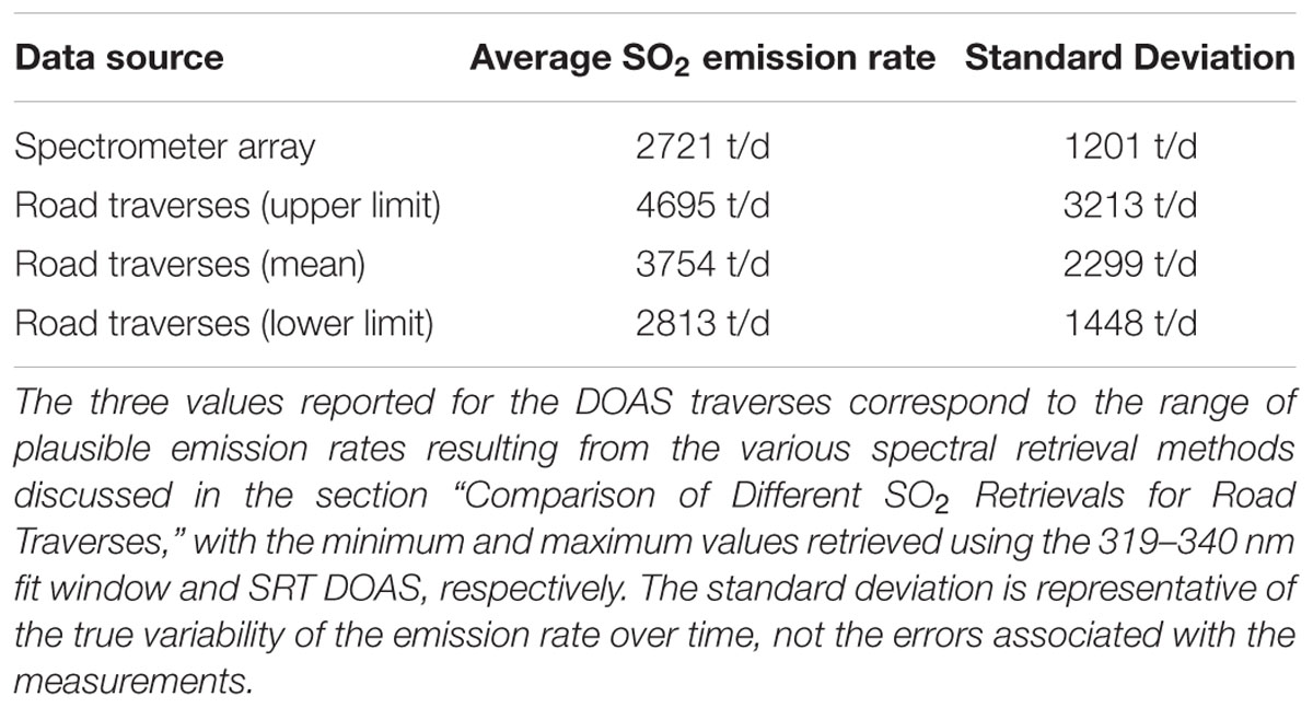
Table 3. Summary of average emission rates obtained from the array and by DOAS vehicle traverses on Crater Rim Drive between 11:05 and 11:52 HST on 30 March 2017.
Figure 12 presents a general comparison of FLYSPEC array and road traverse daily average emission rates from 2014 to 2017 separated into spattering and non-spattering lava lake conditions. A non-spattering lake condition is defined by relative seismic amplitude (RSAM) < 100 counts (see section “SO2 Short-Term Variability Reflects Lava Lake Dynamics”). The traverse data were collected and analyzed using a mobile FLYSPEC and DFW algorithm, or mobile DOAS and extended fit-window (319–340 nm); each traverse took 3–5 min to collect. These data show that on average, the road-based method returns emission rates that are about 60% less than those calculated from the FLYSPEC array for both the spattering and non-pattering cases. While the non-spattering lava lake condition produces a more translucent and gas-poor plume (Patrick et al., 2018), and errors due to radiative transfer effects should have less impact on calculated column densities, the data for both lava lake conditions are not significantly different. Maximum column densities for the non-spattering condition are still greater than 2500 ppmm, so the less opaque plume associated with more quiescent lake conditions can still cause significant errors in retrieved column amounts due to scattering effects. Although on average the road traverse data significantly underestimates emission rates as compared to the FLYSPEC array, as shown in the specific examples in this study, cases of parity, and even traverse values greater than array values do occur. This supports the general observation that the multiple uncertainties impacting the summit road-based data set are difficult to resolve.
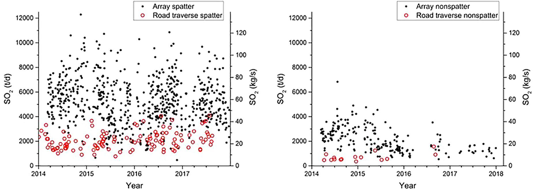
Figure 12. Emission rates from FLYSPEC array (black dots) and road traverses (red circles) separated into spattering (Left) and non-spattering (Right) lava lake conditions. On average, the road-based method returns emission rates that are about 60% less than those calculated from the FLYSPEC array for both lava lake conditions. Non-spattering episodes are defined by RSAM level < 100 counts.
Comparison of Array Emission Rates With Space-Based SO2 Measurements
The array emission rates agree well with OMI space based SO2 measurements. For 2014–2017, Kīlauea released an average of 5100 t/d, or 1.9 ± 0.1 Tg/yr according to array DFW results. This is consistent with Carn et al. (2017) who calculate a daily average of 5518 t/d for Kīlauea for the same period (Carn, 2018, pers. comm., 1 october).
Conclusion and Future Work
Long-lasting eruptions at the summit and East Rift Zone of Kīlauea Volcano have provided a testing ground for novel gas measurement techniques. Traditional SO2 UV spectroscopy measurements via road traverses, performed 10 km downwind of the East Rift Zone eruption accurately measure the generally low emissions from this area. However, the dense volcanic plume produced by the summit lava lake was challenging to quantify using traditional traverse or scanning measurements. Summit emissions during the reported period were best measured using an array of 10 upward looking UV spectrometers (FLYSPECs) spanning the width of the plume ∼3 km downwind of the vent. The FLYSPEC array provides 10-s SO2 emission rate data during daylight hours and prevailing trade wind conditions. To validate these novel measurements, we examined both column density values and calculated emission rates from the array. For column densities, we compared a variety of retrieval techniques with the array’s dual fit window (305–315 and 319.5–330 nm) approach. Comparing fits from (1) conventional DOAS 310–325 nm window, (2) 319–340 nm extended wavelength window, (3) 307–340 nm sliding lower bound (SLFB) window, and (4) Simulated Radiative Transfer DOAS treatment, we found the various methods returned column densities from -6 to +22% of the array values. We consider these results to confirm the validity of the FLYSPEC dual fit window treatment.
To confirm the emission rate values, we investigated the wind and plume speed measurements used to calculate emission rates. We found 3 m agl wind speeds adjacent to the array to be 22% less on average than plume speeds measured with 2 spectrometers located along the plume axis. Thus, the SO2 summit emission rates calculated using the ground-based wind speeds have been adjusted to account for this discrepancy.
Comparing array measurements with helicopter-traverses performed 3 and 6 km downwind of the vent show broad agreement with coincident array measurements with some notable outliers. Helicopter traverse measurements analyzed using a comparable fit window were within +24 and +55% of the array measurements. This discrepancy reflects the underestimation by the array due to the plume maxima being positioned between sensors, as well as the dynamic nature of the plume, differences in time base, viewing angle, and uncertainty of the wind speed for the downwind plume.
Our 1-day detailed case study comparing emission rates from the FLYSPEC array and road traverses shows reasonable agreement (Figure 11). However, the accuracy of the road-based measurements is severely limited by the large discrepancy found between results from different spectral retrieval methods (-30 to +100%, Figure 8). Looking at a longer time series comparison of emission rates shows that the road traverse results differ from the array emission rate values, on average, by a factor of ∼2.5 when using similar retrieval methods for both analyses. The multiple errors for the road-traverse data due to radiative transfer, plume geometry, and wind speed uncertainties create challenging measurement conditions which are difficult to address. The use of SRT-DOAS retrievals can help address the radiative transfer effects for the road data, but the dynamic nature and variable geometry of the plume as well as varying meteorological conditions during the 2014–2017 period creates challenges in the practical application of SRT-DOAS. We surmise that the accuracy of the road-data is insufficient to quantitatively validate the array emission rates for the period in question.
Agreement between SO2 emissions measured from space by OMI and the FLYSPEC array for 2014–2017 are exceptionally good. Daily SO2 values for the two datasets are 5518 t/d and 5100 t/d, respectively. The discrepancy of < 10% between the techniques suggests that space-based emission rates calculated using the new OMI planetary boundary layer SO2 column dataset is a good option for tracking emission rates during periods of vigorous outgassing at Kīlauea.
Technical issues contribute to uncertainties in the array SO2 measurements which could be considered for the future. These include improvements in plume speed calculation, calibration spectra, computer time synchronization, real-time emission rate filters, and spatial resolution of plume features as discussed below.
Plume speed: plume speeds are generated every 1.5 min, or ground based wind speed reported every 10 min, while 1-s column densities are used to calculate 10 s emission rates. The short-term variability in plume motion may not be captured by this treatment. Calibration spectra: we show that column densities retrieved with the array DFW are consistent with conventional and novel fit window comparisons; however, the reference and cell calibration spectra used for these fits could more accurately represent the conditions during sample spectra collection. Since the array is generally in the volcanic plume, there are limited opportunities to collect new calibration spectra for use in analyzing sample spectra. Exploring the use of synthetic reference spectra or use of the conventional modeled DOAS approach could be considered. Time synchronization: accurate and reliable emission rates, and importantly, plume speed calculations, depend on the synchronization of the 10 computer clocks. A robust algorithm for in situ clock checks is critical for accurate emission rate calculations. Emission rate filters: with the large number of instruments and high rate of data collection, spurious data points can occur due to time of day/sun angle and spectrometer inconsistencies. More refined real-time data could be achieved through improved emission rate filtering algorithms. Plume features: spatial resolution could be improved by incorporating scanning spectrometers with ≤ 45° scan angle. While this would provide more plume structure detail and could help avoid missing major plume features passing between stations, it would significantly increase the complexity and cost of the system.
The FLYSPEC array approach may be useful for other volcano observatories requiring high time resolution emission rate measurements. Advantages of the approach include straightforward measurements due to the simple upward looking geometry. The system is particularly useful in locations with a prevailing plume direction coupled with low altitude, inaccessible, or optically dense plumes. Depending on plume column densities, the array can be located at a distance downwind to minimize errors due to light scattering but provide sufficient signal for accurate retrievals. The dual window approach allows flexibility in retrieving variable column amounts accurately and thus can accommodate changes in eruptive activity and outgassing vigor. Disadvantages include the expense and challenge of maintaining multiple field spectrometer systems, the need for robust telemetry, and reduced spatial resolution as compared to scanning systems.
Author Contributions
TE collected, analyzed, and interpreted data, contributed to development of FLYSPEC array hardware and software, prepared manuscript. CK collected, analyzed, and interpreted data, co-wrote manuscript. KH and HG developed FLYSPEC array system, analyzed data, contributed to manuscript. AS collected and analyzed data, contributed to development of FLYSPEC array hardware and software.
Conflict of Interest Statement
KH does business as FLYSPEC, Inc., and sells spectrometer systems.
The remaining authors declare that the research was conducted in the absence of any commercial or financial relationships that could be construed as a potential conflict of interest.
Acknowledgments
Past and current HVO Volunteers Mike Cappos, Gail Ferguson, Howard Hoshide, Isabelle Taylor, Anne Fulton, Tracee Fukunaga, Mary Barr, Jennifer Lennon, and Lora Beatty are deeply thanked for assistance in field data collection and analysis. Thanks to Matt Patrick and Russell Atkinson for programming help, and Matt Patrick for valuable discussion. The Institute of Advanced Studies and the Durham COFUND fellowship scheme (funded by Durham University, United Kingdom, and the European Union) are thanked for providing the opportunity for this manuscript to come to fruition. Authors would also like to acknowledge that this work is conducted inside Hawai‘i Volcanoes National Park with permission from the National Park Service. Any use of trade, firm, or product names is for descriptive purposes only and does not imply endorsement by the U.S. Government.
Supplementary Material
The Supplementary Material for this article can be found online at: https://www.frontiersin.org/articles/10.3389/feart.2018.00214/full#supplementary-material
References
Aiuppa, A., Federico, C., Giudice, G., Gurrieri, S., Liuzzo, M., Shinohara, H., et al. (2006). Rates of carbon dioxide plume degassing from Mount Etna volcano. J. Geophys. Res. 111:B09207. doi: 10.1029/2006JB004307
Andres, R., Kyle, P. R., Stokes, J. B., and Rose, W. I. (1989). SO2 from episode 48A eruption, Hawaii: sulfur dioxide emissions from the episode 48A East Rift Zone eruption of Kilauea volcano, Hawaii. Bull. Volcanol. 52, 113–117. doi: 10.1007/BF00301550
Beirle, S., Horman, C., Penning de Vries, M., Dorner, S., Kern, C., and Wagner, T. (2013). Estimating the volcanic emission rate and atmospheric lifetime of SO2 from space: a case study for Kīlauea Volcano, Hawai‘i. Atmos. Chem. Phys. Discuss. 13:28631. doi: 10.5194/acpd-13-28695-2013
Beirle, S., Hörmann, C., Penning de Vries, M., Dörner, S., Kern, C., and Wagner, T. (2014). Estimating the volcanic emission rate and atmospheric lifetime of SO2 from space: a case study for Kilauea volcano, Hawai‘i. Atmos. Chem. Phys. 14, 8309–8322. doi: 10.5194/acp-14-8309-2014
Bluth, G. J. S., Shannon, J. M., Watson, M., Prata, A. J., and Realmuto, V. J. (2007). Development of an ultra-violet digital camera for volcanic SO2 imaging. J. Volcanol. Geothermal Res. 161, 47–56. doi: 10.1016/j.jvolgeores.2006.11.004
Bobrowski, N., Kern, C., Platt, U., Hörmann, C., and Wagner, T. (2010). Novel SO2 spectral evaluation scheme using the 360–390 nm wavelength range. Atmos. Meas. Tech. 3, 879–891. doi: 10.5194/amt-3-879-2010
Bogumil, K., Orphal, J., Homann, T., Voigt, S., Spietz, P., Fleischmann, O. C., et al. (2003). Measurements of molecular absorption spectra with the SCIAMACHY pre-flight model: instrument characterization and reference data for atmospheric remote-sensing in the 230–2380 nm region. J. Photochem. Photobiol. A Chem. 157, 167–184. doi: 10.1016/S1010-6030(03)00062-5
Businger, S., Huff, R., Pattantyus, A., and Horton, K. (2015). Observing and forecasting Vog dispersion from Kīlauea volcano, Hawaii. Bull. Am. Meteorol. Soc. 96, 1667–1686. doi: 10.1175/BAMS-D-14-00150.1
Carlsen, H. K., Hauksdottir, A., Valdimarsdottir, U. A., Gíslason, T., Einarsdottir, G., Runolfsson, H., et al. (2012). Health effects following the Eyjafjallajökull volcanic eruption: a cohort study. BMJ Open 2:e001851. doi: 10.1136/bmjopen-2012-001851
Carn, S. A., Fioletov, V. E., McLinden, C. A., Li, C., and Krotkov, N. A. (2017). A decade of global volcanic SO2 emissions measured from space. Sci. Rep. 7:44095. doi: 10.1038/srep44095
Casadevall, T. J., Stokes, J. B., Greenland, L. P., Malinconico, L. L., Casadevall, J. R., and Furukawa, B. T. (1987). “SO2 and CO2 emission rates at Kilauea Volcano, 1979–1984,” in Volcanism in Hawaii: U.S. Geological Survey Professional Paper 1350, Vol. 1, Chap. 29, eds R. W. Decker, T. L. Wright, and P. H. Stauffer, 771–780. Available at: https://pubs.usgs.gov/pp/1987/1350/
Chartier, T. A., Rose, W. I., and Stokes, J. B. (1988). Detailed record of SO2 emissions from Pu’u ‘O‘o between episodes 33 and 34 of the 1983–86 ERZ eruption, Kilauea, Hawaii. Bull. Volcanol. 50, 215–228. doi: 10.1007/BF01047485
Cronin, S. J., and Sharp, D. S. (2002). Environmental impacts on health from continuous volcanic activity at Yasur (Tanna) and Ambrym, Vanuatu. Int. J. Environ. Health Res. 12, 109–123. doi: 10.1080/09603120220129274
de Moor, J. M., Aiuppa, A., Pacheco, J., Avard, G., Kern, C., Liuzzo, M., et al. (2016). Short-period volcanic gas precursors to phreatic eruptions: insights from Poás Volcano, Costa Rica. Earth Planet. Sci. Lett. 442, 218–227. doi: 10.1016/j.epsl.2016.1002.1056
Delmelle, P., Stix, J., Baxter, P. J., Garcia-Alvarez, J., and Barquero, J. (2002). Atmospheric dispersion, environmental effects and potential health hazard associated with the low-altitude gas plume of Masaya volcano, Nicaragua. Bull. Volcanol. 64, 423–434. doi: 10.1007/s00445-002-0221-6
Edmonds, M., Herd, R. A., Galle, B., and Oppenheimer, C. M. (2003). Automated, high time-resolution measurements of SO2 flux at Sourfriére Hills Volcano, Montserrat. Bull. Volcanol. 65, 578–586. doi: 10.1007/s00445-003-0286-x
Eguchi, K., Uno, I., Yumimoto, K., Takemura, T., Nakajima, T. Y., Uematsu, M., et al. (2011). Modulation of cloud droplets and radiation over the North Pacific by sulfate aerosol erupted from Mount Kilauea. Sola 7, 77–80. doi: 10.2151/sola.2011-020
Elias, T., Kern, C., Horton, K. A., Garbeil, H., and Sutton, A. J. (2018). SO2 Emission Rates from Kilauea Volcano, Hawaii (2014-2017). Washington, DC: U.S. Geological Survey data Release, doi: 10.5066/F7794402
Elias, T., and Sutton, A. J. (2002). Sulfur Dioxide Emission Rates of Kīlauea Volcano, Hawai‘i, an Update: 1998–2001. U.S. Geological Survey Open-File Report 02–460, 29. Available at: https://pubs.usgs.gov/of/2002/of02-460/
Elias, T., and Sutton, A. J. (2007). Sulfur Dioxide Emission Rates from Kīlauea Volcano, Hawai‘i, an Update: 2002–2006. U.S. Geological Survey Open-File Report 2007–1114, Version 1.0, 37. Available at: https://pubs.usgs.gov/of/2007/1114/
Elias, T., and Sutton, A. J. (2012). Sulfur Dioxide Emission Rates from Kīlauea Volcano, Hawai‘i, 2007–2010. U.S. Geological Survey Open-File Report 2012–1107, 25. Available at: https://pubs.usgs.gov/of/2012/1107/
Elias, T., and Sutton, A. J. (2017). Volcanic Air Pollution Hazards in Hawaii. U.S. Geological Survey Fact Sheet 2017–3017. Available at: https://pubs.er.usgs.gov/publication/fs20173017
Elias, T., Sutton, A. J., Oppenheimer, C., Horton, K. A., Garbeil, H., Tsanev, V., et al. (2006). Comparison of COSPEC and two miniature ultraviolet spectrometer systems for SO2 measurements using scattered sunlight. Bull. Volcanol. 68, 313–322. doi: 10.1007/s00445-005-0026-5
Elias, T., Sutton, A. J., Stokes, J. B., and Casadevall, T. J. (1998). Sulfur Dioxide Emission Rates of Kīlauea Volcano, Hawai‘i, 1979–1997. U.S. Geological Survey Open-File Report 98–462. Available at: http://pubs.usgs.gov/of/1998/of98-462/
Fickel, M., and Delgado Granados, H. (2017). On the use of different spectral windows in DOAS evaluations: effects on the estimation of SO2 emission rate and mixing ratios during strong emission of Popocatépetl volcano. Chem. Geol. 462, 67–73. doi: 10.1016/j.chemgeo.2017.05.001
Galle, B., Johansson, M., Rivera, C., Zhang, Y., Kihlman, M., Kern, C., et al. (2010). Network for observation of volcanic and atmospheric change (NOVAC): a global network for volcanic gas monitoring: network layout and instrument description. J. Geophys. Res. 115:D05304. doi: 10.1029/2009JD011823
Galle, B., Oppenheimer, C., Geyer, A., McGonigle, A. J. S., Edmonds, M., and Horrocks, L. (2003). A miniaturized ultraviolet spectrometer for remote sensing of SO2 fluxes: a new tool for volcano surveillance. J. Volcanol. Geothermal Res. 119, 241–254. doi: 10.1016/S0377-0273(02)00356-6
Gerlach, T. M., McGee, K. A., Sutton, A. J., and Elias, T. (1998). Rates of volcanic CO2 degassing from airborne determinations of SO2 emission rates and plume CO2/SO2: test study at Pu’u ’O’o cone, Kilauea volcano, Hawaii. Geophys. Res. Lett. 25, 2675–2678. doi: 10.1029/98GL02030
Gliß, J., Stebel, K., Kylling, A., and Sudbø, A. (2018). Improved optical flow velocity analysis in SO2 camera images of volcanic plumes – implications for emission-rate retrievals investigated at Mt Etna, Italy and Guallatiri, Chile. Atmos. Meas. Tech. 11, 781–801. doi: 10.5194/amt-11-781-2018
Global Volcanism Program (2014). “Report on Kilauea (United States),” in Bulletin of the Global Volcanism Network, Vol. 39, ed. R. Wunderman (Washington, DC: Smithsonian Institution), 12. doi: 10.5479/si.GVP.BGVN201412-332010
Grainger, J. F., and Ring, J. (1962). A photoelectric grating spectrometer. Mon. Not. R. Astron. Soc. 125, 93–104. doi: 10.1093/mnras/125.2.93
Halliday, T. J., Lynham, J., and de Paula, A. (2018). VOG: using volcanic eruptions to estimate the health costs of particulates. Econ. J. doi: 10.1111/ecoj.12609
Halmer, M. M., Schmincke, H.-U., and Graf, H.-F. (2002). The annual volcanic gas input into the atmosphere, in particular into the stratosphere: a global data set for the past 100 years. J. Volcanol. Geothermal Res. 115, 511–528. doi: 10.1016/S0377-0273(01)00318-3
Horton, K. A., Garbeil, H., Sutton, A. J., Elias, T., and Businger, S. (2012). “Early monitoring results from the Halema‘uma‘u vog measurement and prediction FLYSPEC array,” in Proceedings of the Conferences on Extended Abstracts, AGU Chapman Hawaiian Volcanoes: From Source to Surface, (Waikoloa, HI: American Geophysical Union).
Horton, K. A., Williams-Jones, G., Garbeil, H., Elias, T., Sutton, A. J., Mouginis-Mark, P., et al. (2006). Real-time measurement of volcanic SO2 emissions: validation of a new UV correlation spectrometer (FLYSPEC). Bull. Volcanol. 68, 323–327. doi: 10.1007/s00445-005-0014-9
Kern, C., Deutschmann, T., Werner, C., Sutton, A. J., Elia, T., and Kelly, P. J. (2012). Improving the accuracy of SO2 column densities and emission rates obtained from upward-looking UV-spectroscopic measurements of volcanic plumes by taking realistic radiative transfer into account. J. Geophys. Res. 117:D20302. doi: 10.1029/2012JD017936
Kern, C., Kick, F., Lübcke, P., Vogel, L., Wöhrbach, M., and Platt, U. (2010). Theoretical description of functionality, applications, and limitations of SO2 cameras for the remote sensing of volcanic plumes. Atmos. Meas. Tech. 3, 733–749. doi: 10.5194/amt-3-733-2010
Kern, C., Sutton, J., Elias, T., Lee, L., Kamibayashi, K., Antolik, L., et al. (2015). An automated SO2 camera system for continuous, real-time monitoring of gas emissions from Kīlauea Volcano’s summit Overlook Crater. J. Volcanol. Geothermal Res. 300, 81–94. doi: 10.1016/j.jvolgeores.2014.12.004
Kern, C., Werner, C., Elias, T., Sutton, A. J., and Lubcke, P. (2013). Applying UV cameras for SO2 detection to distant or optically thick volcanic plumes. J. Volcanol. Geothermal Res. 262, 80–89. doi: 10.1016/j.jvolgeores.2013.06.009
Klein, A., Lübcke, P., Bobrowski, N., Kuhn, J., and Platt, U. (2017). Plume propagation direction determination with SO2 cameras. Atmos. Meas. Tech. 10, 979–987. doi: 10.5194/amt-10-979-2017
Mather, T. A., Pyle, D. M., Tsanev, V. I., McGonigle, A. J. S., Oppenheimer, C., and Allen, A. G. (2006). A reassessment of current volcanic emissions from the Central American arc with specific examples from Nicaragua. J. Volcanol. Geothermal Res. 149, 297–311. doi: 10.1016/j.jvolgeores.2005.07.021
Millan, M. M. (1980). Remote sensing of air pollutants. A study of some atmospheric scattering effects. Atmos. Environ. 14, 1241–1253. doi: 10.1016/0004-6981(80)90226-7
Millán, M. M., and Chung, Y. S. (1977). Detection of a plume 400 km from the source. Atmos. Environ. 11, 939–944. doi: 10.1016/j.jconhyd.2010.09.009
Moffat, A. J., and Millan, M. M. (1971). The application of optical correlation techniques to the remote sensing of SO2 plumes using skylight. Atmos. Environ. 5, 677–690. doi: 10.1016/0004-6981(71)90125-9
Moré, J. (1978). “The levenberg-marquardt algorithm: implementation and theory,” in Numerical Analysis, Vol. 630, ed. G. A. Watson (Berlin: Springer-Verlag).
Mori, T., Hirabayashi, J., Kazahaya, K., Mori, T., Ohwada, M., Miyashita, M., et al. (2007). A Compact Ultraviolet Spectrometer System (COMPUSS) for monitoring volcanic SO2 emission: validation and preliminary observation. Bull. Volcanol. Soc. Jan. 52, 105–112.
Mori, T., Mori, T., Kazahaya, K., Ohwada, M., Hirabayashi, J., and Yoshikawa, S. (2006). Effect of UV scattering on SO2 emission rate measurements. Geophys. Res. Lett. 33:L17315. doi: 10.1029/2006GL026285
Nadeau, P. A., Werner, C. A., Waite, G. P., Carn, S. A., Brewer, D., Elias, T., et al. (2015). Using SO2 camera imagery and seismicity to examine degassing and gas accumulation at Kīlauea Volcano, May 2010. J. Volcanol. Geothermal Res. 300, 70–80. doi: 10.1016/j.jvolgeores.2014.12.005
Oppenheimer, C., Scaillet, B., Woods, A., Sutton, A. J., Elias, T., and Moussallam, Y. (2018). Influence of eruptive style on volcanic gas emission chemistry and temperature. Nat. Geosci. 11, 678–681. doi: 10.1038/s41561-018-0194-5
Patrick, M., Orr, T., Sutton, J. A., Elias, T., and Swanson, D. (2013). The First Five Years of Kīlauea’s Summit Eruption in Halema‘uma‘u Crater, 2008–2013: U.S. Geological Survey Fact Sheet 2013–3116. Available at: https://pubs.er.usgs.gov/publication/fs20133116
Patrick, M. R., Orr, T., Sutton, A. J., and Lev, E. (2016a). Shallow and deep controls on lava lake surface motion at Kīlauea Volcano. J. Volcanol. Geothermal Res. 328, 247–261. doi: 10.1016/j.jvolgeores.2016.11.010
Patrick, M. R., Orr, T., Sutton, A. J., Lev, E., Thelen, W., and Fee, D. (2016b). Shallowly driven fluctuations in lava lake outgassing, Kīlauea Volcano, Hawai‘i. Earth Planet. Sci. Lett. 433, 326–338. doi: 10.1016/j.epsl.2015.10.052
Patrick, M. R., Orr, T., Swanson, D., Elias, T., and Shiro, B. (2018). Lava Lake Activity at the Summit of Kīlauea Volcano in 2016: U.S. Geological Survey Scientific Investigations Report 2018–5008, 58. Available at: https://pubs.er.usgs.gov/publication/sir20185008
Perner, D., and Platt, U. (1979). Detection of nitrous acid in the atmosphere by differential optical absorption. Geophys. Res. Lett. 7, 1053–1056. doi: 10.1029/GL007i012p01053
Peters, N., Hoffmann, A., Barnie, T., Herzoga, M., and Oppenheimer, C. (2015). Use of motion estimation algorithms for improved flux measurements using SO2 cameras. J. Volcanol. Geothermal Res. 300, 58–69. doi: 10.1016/j.jvolgeores.2014.08.031
Platt, U. (1994). “Differential optical absorption spectroscopy (DOAS),” in Air Monitoring by Spectroscopic Techniques Chemical Analysis Series, Vol. 127, ed. M. W. Sigrist (Hoboken, NJ: Wiley), 27–84.
Platt, U., and Stutz, J. (2008). Differential Optical Absorption Spectroscopy - Principles and Applications. Berlin: Springer. doi: 10.1007/978-3-540-75776-4
Robock, A. (2000). Volcanic eruptions and climate. Rev. Geophys. 38, 191–219. doi: 10.1029/1998RG000054
Stoiber, R. E., Malinconico, L. L., and Williams, S. N. (1983). “Use of the correlation spectrometer at volcanoes,” in Forecasting Volcanic Events, eds H. Tazieff and J. C. Sabroux (Amsterdam: Elsevier), 424–444.
Sutton, A. J., and Elias, T. (2014). “One hundred volatile years of volcanic gas studies at the Hawaiian Volcano Observatory,” in U.S. Geological Survey Professional Paper 1801, (Reston, VA: USGS).
Sutton, A. J., Elias, T., Gerlach, T. M., and Stokes, J. B. (2001). Implications for eruptive processes as indicated by sulfur dioxide emissions from Kilauea Volcano, Hawai‘i, 1979-1997. J. Volcanol. Geothermal Res. 108, 283–302. doi: 10.1016/S0377-0273(00)00291-2
Symonds, R. B., Rose, W. I., Bluth, G. J. S., and Gerlach, T. M. (1994). “Volcanic-gas studies: methods, results, and applications,” in Volatiles in Magmas, eds M. R. Carroll and J. R. Hollaway (Chantilly, VA: Mineralogical Society of America), 1–66.
Tam, E., Miike, R., Labrenz, S., Sutton, A. J., Elias, T., Davis, J., et al. (2016). Volcanic air pollution over the Island of Hawai‘i; emissions, dispersal, and composition. Association with respiratory symptoms and lung function in Hawai‘i Island school children. Environ. Int. 92–93, 543–552. doi: 10.1016/j.envint.2016.03.025
Uno, Eguchi, K., and Yumimoto, K. (2013). “Eruption of Mt. Kilauea impacted cloud droplet and radiation budget over North Pacific,” in Western Pacific Air-Sea Interaction Study, eds M. Uematsu, Y. Yokouchi, Y. W. Watanabe, S. Takeda, and Y. Yamanaka (Tokyo: TERRAPUB), 83–87.
van Manen, S. (2014). Perception of a chronic volcanic hazard: persistent degassing at Masaya volcano, Nicaragua. J. Appl. Volcanol. 3:1. doi: 10.1186/s13617-014-0009-3
Vandaele, A. C., Hermans, C., and Fally, S. (2009). Fourier transform measurements of SO2 absorption cross sections: II. Temperature dependence in the 29 000–44 000 cm-1 (227–345 nm) region. J. Quant. Spectrosc. Radiat. Transf. 110, 2115–2126. doi: 10.1016/j.jqsrt.2009.05.006
Wilson, D., Elias, T., Orr, T., Patrick, M., Sutton, J., and Swanson, D. (2008). Small explosion from new vent at Kilauea’s summit. Eos Trans. Am. Geophys. Union 89:203. doi: 10.1029/2008EO220003
Keywords: sulfur dioxide, Kīlauea, emission rate, DOAS, FLYSPEC
Citation: Elias T, Kern C, Horton KA, Sutton AJ and Garbeil H (2018) Measuring SO2 Emission Rates at Kīlauea Volcano, Hawaii, Using an Array of Upward-Looking UV Spectrometers, 2014–2017. Front. Earth Sci. 6:214. doi: 10.3389/feart.2018.00214
Received: 18 August 2018; Accepted: 05 November 2018;
Published: 17 December 2018.
Edited by:
Alessandro Aiuppa, Università degli Studi di Palermo, ItalyReviewed by:
Dmitri Rouwet, Istituto Nazionale di Geofisica e Vulcanologia, ItalyMarie Edmonds, University of Cambridge, United Kingdom
Copyright © 2018 Elias, Kern, Horton, Sutton and Garbeil. This is an open-access article distributed under the terms of the Creative Commons Attribution License (CC BY). The use, distribution or reproduction in other forums is permitted, provided the original author(s) and the copyright owner(s) are credited and that the original publication in this journal is cited, in accordance with accepted academic practice. No use, distribution or reproduction is permitted which does not comply with these terms.
*Correspondence: Tamar Elias, telias@usgs.gov