The scaling of experiments on volcanic systems
 Olivier Merle
- Laboratoire Magmas et Volcans, Université Blaise Pascal - Centre National de la Recherche Scientifique - IRD, Clermont Ferrand, France
In this article, the basic principles of the scaling procedure are first reviewed by a presentation of scale factors. Then, taking an idealized example of a brittle volcanic cone intruded by a viscous magma, the way to choose appropriate analog materials for both the brittle and ductile parts of the cone is explained by the use of model ratios. Lines of similarity are described to show that an experiment simulates a range of physical processes instead of a unique natural case. The pi theorem is presented as an alternative scaling procedure and discussed through the same idealized example to make the comparison with the model ratio procedure. The appropriateness of the use of gelatin as analog material for simulating dyke formation is investigated. Finally, the scaling of some particular experiments such as pyroclastic flows or volcanic explosions is briefly presented to show the diversity of scaling procedures in volcanology.
Introduction
From as early as the beginning of the nineteenth century, scientists have reproduced geological deformations in the laboratory. The oldest experimental study was performed by James Hall who recreated the folding of sedimentary strata by horizontal compression (Hall, 1815). Following Hall, a few other important works were carried out during the nineteenth century (e.g., Daubrée, 1879; Cadell, 1889; Willis, 1891/1892; Reyer, 1892). While the experimental approach continued in the first part of the twentieth century (e.g., Sollas, 1906; Cloos, 1928, 1955; Bucher, 1956), it remained rather episodic during that period.
It was in the early seventies that a revival in scaled modeling occurred through Ramberg's work at the Upsala experimental laboratory in Sweden. A key point in this recovery was the serious guarantee offered by Ramberg about the scaling of experiments, as detailed in his famous book which was first edited in 1969 (Ramberg, 1981). Following this impetus, other European universities set up experimental laboratories, like Imperial College in London, and the Geosciences Rennes laboratory in Rennes, which has conducted a huge amount of experimental studies on tectonic structures. Since then, experimental studies have earned their credentials, being acknowledged as a useful tool to understand geological processes.
The scaling of experiments is one of the main criticisms addressed by skeptics toward this scientific approach. Barenblatt (1996) writes that in the past “the dimensional analysis was cursed and reproached for being untrustworthy and unfounded, even mystical.” He adds that the reason for this skepticism is that just a few people really understood the content and true abilities of dimensional analysis. However, the general principles of scaling are quite simple and, if an experiment is well scaled, it has a good chance of providing useful insights into the physical evolution of the studied problem.
Due to the surge of experimental studies in volcanology over the last 20 years or so, it seems useful to detail the strengths and the weaknesses of this approach. The aim of this article is to present a kind of review and reappraisal of the scaling procedure. A simple example is taken to illustrate the procedure in a concrete way. A few other examples also show that the scaling procedure may be quite different according to the different volcanic systems studied by the experimenter.
The Goal of Scaled Models
The goal of scaled modeling is not to reproduce a specific natural example. What the experimenter wants to understand is the evolution through time of a physical system. The basic hypothesis is that the model simulates the evolution of the natural prototype in a way which is convenient to the observer, that is of short duration and small geometric scale.
The experimenter must define the main characteristics of the physical system he wants to investigate. Then, he must build up an experimental device which is as simple as possible. The set-up is merely an idealized version of the original. The conceptualization, by definition, is far from any specific natural case. The model is a simplification of the reality because the latter cannot be understood in all aspects of its deep complexity.
Usually, the experimenter tries to understand the role of a limited numbers of parameters in the evolution of the system. These parameters are closely dependent on the experiment itself and can be geometric, kinematic and/or dynamic. Each experiment is carried out at least twice to verify its reproducibility. Only one parameter must be changed for each new experiment to establish its specific role.
However, it would be hypocritical to deny that most experimenters have a specific natural case in mind when preparing a set of experiments, and in some case they may try to reproduce a specific scenario, timing and event. It is the field data that raise the geological problems, then the hypothetical solutions of these problems that generate ideas to make new experiments. A good experimenter is one who searches, beyond the specific natural case, for the universal laws that govern the physical system.
The Basic Principles
Two articles must be considered together as milestones in the history of experimental geology. Ampferer (1906) noted that, as lengths are reduced in a model, all other “constants” should also be reduced accordingly, like stiffness, flexibility and strength. Shortly after, Koenigsberger and Morath (1913) discussed the scale reduction in terms of the three fundamental units: length, mass, and time. Indeed, a scaled model is intended to be geometrically, kinematically, and dynamically similar to nature (e.g., Hubbert, 1937; Ramberg, 1981). This has important consequences for the building of scaled models. Scale factors must be defined. A scale factor is the ratio between a characteristic parameter in both the model and the original. Knowing the value of the parameter in the original, the same parameter must be scaled down in the model according to the scale factor.
The model is said to be geometrically similar if it is a geometric replica on a smaller scale to the natural system, which serves as the prototype or original. This means that the ratio between the corresponding distances in the model and the original is constant for a given model-original pair. This allows the definition of the length ratio (h*) between model and original:
where the subscripts m and n refer to model and nature, respectively.
The model is said to be kinematically similar if it remains geometrically similar to nature during the deformation. To fulfill this condition, a time ratio (t*) must be defined:
The time ratio is the ratio between the time needed to complete an intermediate movement in the model and the time to complete the corresponding intermediate movement in the original. The time ratio must remain constant during the total duration of the experiment from start to finish.
In reality, it is impossible to define this time ratio because the evolution of the physical process through time is unknown, so we cannot ensure that the time ratio remains constant at each stage of the deformation. However, by fixing the duration of the experiments, a time ratio (t*) can be defined if we have a rough estimate of the time needed in nature to complete the total deformation. In that case, the model is kinematically similar only if it is also dynamically similar to nature.
A model is said to be dynamically similar to nature if the ratio between mechanical forces in the model and in the prototype, compared kind for kind, is constant:
where the subscripts g, i, μ, and f refer to gravity, inertia, viscous, and frictional force, respectively. Of course, forces in the model and in the prototype must also have the same direction. Equation (3) has an important implication. It means that the mass ratio (m*) must be constant for corresponding volume throughout the model and original. Indeed, the ratio of body forces, for example inertia or gravity, cannot be constant if the ratio of mass is not. So, after h* and t*, a third important ratio is defined which ensures the mechanical similarity of the model:
Accordingly, the three model ratios, which allow a model to be well scaled, are length, time and mass ratios. Length [L], time [T], and mass [M] are three basic concepts in mechanics. All other concepts such as force [MLT−2], velocity [LT−3], viscosity [ML−1T−1], density [ML−3], stress [ML−1T−2], etc., are defined from these three fundamental dimensions. Likewise, all model ratios related to mechanical concepts and useful in the scaling procedure can be defined from model ratios of length (h*), time (t*), and mass (m*).
The Use of Scale Factors
These basic principles are enough to scale a model. Once the size of the model is chosen, a length ratio (h*) can be defined. Knowing the density of the rocks in the prototype, the density of the analog material allows the definition of a density ratio (d*). Finally, a stress ratio (σ*) may be defined from gravity stresses exerted in the model and the original:
where g* is the ratio between the gravitational acceleration in the model and the original. g* = 1 if no centrifuge is used for the experiment. The density of natural and analog materials varies only by a small amount. It follows that Equation (5) may simplify to σ* ≈ h*, which explains why many authors scale down quantities with a dimension of stress by the same factor as the linear dimensions (e.g., Hubbert, 1945; Davy and Cobbold, 1988; Brun, 1999).
Brittle Materials
The deformation of brittle materials is rate-independent, meaning that the same deformation in the model is achieved whatever the strain rate. Brittle materials are characterized by two constants: the cohesive shear strength, or cohesion (τ0), and the angle of internal friction (ϕ).
The cohesion has the dimension of a stress, so the cohesion (τ0m) of the brittle analog material must be scaled down by the same factor as the gravity stress.
The angle of internal friction is a dimensionless number. It must be identical (or close) in both the analog material and the volcano:
Ductile Materials
The scaling of ductile material is more challenging. The deformation of ductile material is rate-dependent and the strain rate strongly influences the whole deformation. We need to determine the viscosity of the analog material. The strain rate ratio (e*) is related to time and viscosity by the following relations:
As σ* = ρ*g*h*, the viscosity ratio (μ*) is:
Hubbert has shown that this equation is the basic one to scale models where gravity is the only significant force at work in the model (Hubbert, 1937). This ensures both dynamic and geometric similarity in experiments. If we have a reasonable knowledge of the duration of the deformation in nature, and given the fact that the duration of an experiment is often fixed to a few hours for practical convenience, the viscosity in the model is calculated from the viscosity in nature. The last point is the most tricky. Estimates of viscosity in a specific natural case may vary by one or two (or more) orders of magnitude, depending on the authors. So, the value of the natural viscosity (μn) chosen to scale the model is a bit speculative. This uncertainty means that a scaled model can only simulate a general physical process rather than a specific field example. We return to this point later.
The velocity [LT−1] being the ratio between length and time, the velocity ratio for any displacement in the model is simply:
Of course, the direction of corresponding velocity vectors in the model and the prototype must be the same.
The Choice of Analog Materials
To illustrate the method of scale ratio, we take the example of a simple volcanic cone vertically intruded by magma (Figure 1). The aim of the experiment could be the study of the cone deformation during the ascent of the magma (e.g., Donnadieu and Merle, 1998).
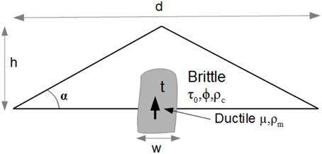
Figure 1. Idealized example of ductile magma intruding a brittle cone. τ0, ϕ, ρc are the cohesion, the angle of internal friction and the density of the brittle cone, respectively. μ and ρm are the viscosity and the density of the magma, respectively. t is the time span for deformation.
Starting from scratch, it is convenient to use Equation (5). Unless a centrifuge is used, experiments are conducted in the Earth's gravity field (g* = 1). The analog materials used in this type of experiment are granular materials. The density of granular materials is generally half that of rocks so that the density ratio ρ* is close to 0.5 (e.g., Schellart, 2000). The height of the model is about 10 cm, which is a convenient height for the observer. Then the length ratio (h*) is about 10−4 if we plan to study a thousand meter high volcano (1 cm in the model represents 100 m in nature). In such a case, σ* = 5 × 10⁻⁵. This means that the model needs to be 20,000 times weaker than the original.
Brittle Material
The cohesion (τ0m) of the analog material can be determined from Equation (6). The difficulty is to assess the cohesion (τ0n) of a volcanic cone. The cohesion of intact rock is about 107 Pa (e.g., Handin, 1966; Jaeger and Cook, 1971). However, the rocks in a volcanic cone are very often intensely fractured and/or deeply altered by hydrothermal activity. The bulk cohesion is potentially lowered by one or two orders of magnitude with respect to intact rocks (e.g., Hoshino et al., 1972; Hoek and Bray, 1981; Schultz, 1996).
Consequently, the cohesion of the analog material can vary from 500 Pa with τ0n = 107 Pa to 5 Pa with τ0n = 105 Pa. This gives a lot of freedom in the choice of analog materials: we can decide to simulate the deformation of a “strong” or a “weak” volcano. There are many granular materials with a low cohesion like plaster, microbeads, flour, sand, etc. Many of them like sand, crystalline silica powder, sugar, corundum, pyrex, siliceous and glass microspheres, have been extensively studied and their mechanical properties including the cohesion and the angle of friction have been measured using shear apparatus (e.g., Krantz, 1991; Cobbold and Castro, 1999; Schellart, 2000; Lohrmann et al., 2003; Mourgues and Cobbold, 2003; Galland et al., 2006; Panien et al., 2006). A practical method to calculate the cohesion of any appropriate dry powder is given in the Appendix A.
The angle of internal friction of natural rocks is about 30–40° (e.g., Byerlee, 1978). According to Equation (7), the analog material must exhibit a similar angle of friction. Note that the angle of repose (α) (i.e., the angle between the surface slope of the cone and the horizontal, Figure 1) of any granular material is considered to be equal to the angle of internal friction (Coulomb, 1776, p. 361; Absi, 1993, p. 94), making it easy to measure when building the cone.
Ductile Material
For practical convenience, the duration of experiments is fixed to a few hours. If geological data give a reasonable approximation of the average duration of the natural process, the time ratio (t*) can be approximated first.
The main difficulty is to determine the viscosity value of the magma in nature. The viscosity of the original may vary greatly from 102/103 Pa s at 1200°C (basaltic magma) to 1011–1012 Pa s at 900°C (acid magma) and even 1015 Pa s for a magma with a high crystal content (e.g., Shaw, 1972; Eichelberger and Hayes, 1982; Murase et al., 1985; Nicolas and Ildefonse, 1996). Clearly, data on magma viscosity in nature are not precise enough to allow the experimenter to simulate a specific natural case. Once again, we model a physical process which operates within a wide range of viscosity varying over several orders of magnitude. This is especially true since viscosity is temperature-dependent, and therefore time-dependent, increasing with time as the magma temperature decreases. The impact on the model evolution due to this uncertainty is difficult to evaluate. The same problem is encountered in numerical simulation.
Whatever this uncertainty on the rock viscosity in nature, the appropriate viscosity needed in the model may be determined from Equation (9):
We can illustrate the order of magnitude of the viscosity (μm) using Figure 1. If g* = 1 (Earth's gravity field), t* = 3.5 × 10⁻³ (for instance a 2 month process in nature simulated in 5 h in the lab), ρ* = 0.5, h* = 10−4 (see above) and μn = 1011 Pa s (silicic magma), then the viscosity in the model should be 1.7 × 10⁵ Pa s to properly simulate the physical process under consideration.
The velocity (vn) of the magma ascent in nature is related to the duration of the deformation, so vn may be calculated from tn. Considering a vertical displacement of one thousand meters in 2 months, vn is about 2× 10⁻⁴ m/s. This slow velocity is in good agreement with a highly viscous magma (μn = 1011 Pas). The velocity in the model may be calculated from Equation (10):
This yields a velocity of 2 cm/h in the model. If the analog magma starts from the base of a cone 10 cm in height, the experiment duration will be about 5 h. This is a practical duration for an experiment. In the lab, the desired velocity for the vertical ascent of the magma analog may be imposed by a computer-controlled motor.
It is interesting to note that more than one ductile material can be used in a single experiment, for instance a low-viscosity layer at the base of the analog volcano and an intruding magma (e.g., Le Corvec and Walter, 2009). Once the time ratio (t*), the length ratio (h*) and the density ratio (ρ*) have been fixed, it follows from Equation (11) that the viscosity ratio (μ* = μm/μn) is a constant. This means that the viscosity ratio for sediments (μ*sd) and the viscosity ratio for magma (μ*mg) must be the same. Scaling these two ductile materials necessitates finding two different analog materials which fulfill the following relation μ* = μm(sd)/μn(sd) = μm(mg)/μn(mg). As it is a difficult task to find such materials, the same analog material is sometimes used for modeling both the weak layer and the magma, and results are considered qualitatively (e.g., Merle and Vendeville, 1995; Le Corvec and Walter, 2009).
Types of Experiments
The scaling procedure that we have examined so far can be applied successfully to volcanic processes using granular materials to reproduce the brittle deformation and viscous fluids (silicone, vegetable oil, honey, golden syrup, etc.) to reproduce the ductile deformation (e.g., Weijermars, 1986).
This mainly concerns experiments like the ascent of the magma within an edifice (our idealized example, e.g., Donnadieu and Merle, 1998), the formation of calderas (e.g., Komuro, 1987; Marti et al., 1994; Odonne et al., 1999; Acocella et al., 2000; Roche et al., 2000; Walter and Troll, 2001; Troll et al., 2002; Holohan et al., 2005; Geyer et al., 2006), volcano core-collapse and hydrothermal calderas (e.g., Van Wyk de Vries et al., 2000; Merle and Lénat, 2003; Cecchi et al., 2005; Merle et al., 2006, 2010; Barde-Cabusson and Merle, 2007), lava flows (e.g., Merle, 1998; Lescinsky and Merle, 2005), volcanic spreading (e.g., Merle and Borgia, 1996; Walter, 2003; Oehler et al., 2005; Walter et al., 2006; Delcamp et al., 2008; Platz et al., 2011; Byrne et al., 2013; Kervyn et al., 2014), volcanic domes (e.g., Buisson and Merle, 2002, 2005; Galland, 2012), resurgent domes (e.g., Acocella et al., 2001; Galland et al., 2009; Marotta and de Vita, 2014; Brothelande and Merle, 2015), magmatic intrusions (e.g., Merle and Vendeville, 1995; Roman-Bierdel et al., 1995; Galland et al., 2009; Galerne et al., 2011), interaction between regional tectonics and volcano deformation (e.g., Tibaldi, 1995; van Wyk de Vries and Merle, 1996, 1998; Lagmay et al., 2000; Branquet and van Wyk de Vries, 2001; Merle et al., 2001; Galland et al., 2003, 2007; Girard and van Wyk de Vries, 2005; Norini and Lagmay, 2005; Tibaldi et al., 2006; Holohan et al., 2008; Tibaldi, 2008; Norini and Acocella, 2011; Le Corvec et al., 2014), dyke, sill and laccolith formation (e.g., Galland et al., 2006; Mathieu et al., 2008; Abdelmalak et al., 2012), etc.
The Use of a Centrifuge
The use of a centrifuge does not change the basic principles of scaling. The difference is that the gravity acceleration is not the same in nature and in the model, so g* ≠ 1. The acceleration of the centrifuge may be about 103 or 104 g (Ramberg, 1971, 1981; Dixon and Summers, 1985) resulting in a gravity ratio g* = 103 or 104. The stress ratio (σ*) is modified. Taking again the example in Figure 1, the stress ratio is increased by three or four orders of magnitude (σ* = 5 × 10⁻² or 5 × 10⁻¹ instead of 5 × 10⁻⁵).
For a brittle material, the cohesion (τ0m) of the analog material is calculated from Equation (6). Accordingly, the cohesion of the brittle material in the example in Figure 1 must be increased by three or four orders of magnitude, which gives τ0m = 5 × 10⁵ or 5 × 10⁶ Pa if τ0n = 107 Pa and τ0m = 5 × 10³ or 5 × 10⁴ Pa if τ0n = 105 Pa. In other words, the material in the experiment must be 1000 or 10,000 times stronger than that for non-centrifuged models.
The advantage of the centrifuge is that it can perform very fast experiments. An experiment can last as little as 15 min (≈ 103 s). The time ratio (t*) is modified. In the example in Figure 1, where the deformation in nature lasts 2 months, t* = 2 × 10⁻⁴ and the viscosity of the analog material (μm) calculated from Equation (11) must be 106 Pa s with g* = 103 or 107 Pa s with g* = 104. Despite the reduction of tm, an increase g in the experiments necessitates using an analog material with a higher viscosity than in non-centrifuged experiments.
Lines of Similarity
Brittle Experiments
Experiments using only brittle materials are rate-independent. The two parameters which must be scaled are the cohesion and the angle of internal friction. Combining Equations (5) and (6), we obtain:
In other words, once model parameters are fixed, the cohesion (τ0m) and the length (hm) in nature are related by a relation of the type:
where a is a constant. Considering a purely brittle experiment where τ0m = 50 Pa and hm = 10−1 m, with g* = 1 and ρ* = 0.5, then a = 103 and Equation (14) yields τ0n = 103 hn. A graph may explain this relationship (Figure 2). It defines a line of similarity, which reveals that a single experiment simulates a range of natural cases that go from big volcanoes (2000 m high) with a relatively strong cohesion (106 Pa) to small volcanoes (100 vm high) with a low cohesion (105 Pa). This result is a clear illustration that experiments do not simulate a specific natural case, but a wider physical process for which Figure 2 gives the application field.
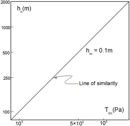
Figure 2. The line of similarity shows the range of cohesion (τ0n) and height (hn) in nature simulated by an experiment with a cone 0.1 m high (hm). Both horizontal and vertical axes have log scales.
Ductile Experiments
Experiments using ductile materials are rate-dependent. This means that time and viscosity are interrelated in nature. If the experiment in Figure 1 had been scaled as shown in the previous section, the experimenter would expect to study the slow ascent of a highly viscous magma within a brittle cone. In reality, the experimenter simulates a wider range of natural conditions.
Rearranging Equation (9), we obtain:
As soon as the duration (tm) and the height of the model are fixed (generally for practical convenience) and the choice of the analog material has been decided on from the scaling procedure, tm, μm, ρ*, and h* are constants in Equation (15). Considering experiments conducted in the Earth's gravity field (g* = 1), Equation (15) is in the form:
where b is a constant. At first sight, this is quite surprising as it reveals that the slow ascent of a highly viscous magma in a volcanic cone is not the only case investigated by the experimenter. As a matter of fact, Equation (16) works for a wide range of pairs of natural times and natural viscosities. These are plotted in Figure 3. Equation (16) allows a line of similarity to be drawn between nature and the model, which provides values for the time of the deformation and the viscosity of the magma in nature. The graph reveals that a single experiment models dynamic systems that range from slow deformation with a high-viscosity magma to very slow deformation with a very high-viscosity magma. As the height of the volcanoes (hm) cannot vary very much in nature, the length ratio h* is not very sensitive in this type of experiment but allows other lines of similarity to be defined (Figure 3).
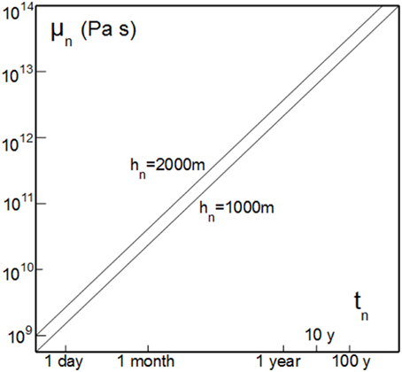
Figure 3. The two lines of similarity for hn = 1000 m and hn = 2000 m show the range of natural viscosities versus natural times simulated by an experiment lasting 5 h (t = 18.000 s) with a cone 0.1 m high (hm). Both horizontal and vertical axes have log scales. The constant b = 19,444 and 38,888 for hn = 1000 and 2000 m, respectively (μm = 1.75 104 Pa s, ρ* = 0.5). Explanation in the text.
Thinking that a model reproduces a specific field example, for which the viscosity and duration are known, would limit the applicability of the model, especially as these natural values are rather speculative. Again, the goal of the experiments is to understand a geological process, regardless of whether it happens by the rapid injection of low-viscosity magma or the slow injection of high-viscosity magma. However, this graph also shows the limitation of the model. The viscosity of the analog material (μm ≈ 104 Pas) does not allow the study of the vertical ascent of a low-viscosity magma (<109 Pa s, Figure 3) within a brittle cone. To do so, another analog material with a lower viscosity is needed (e.g., Galland et al., 2006; Mathieu et al., 2008).
Likewise, Equation (15) can be rewritten to show the relation between the natural viscosity (μn) and the vertical velocity (vn) of the magma:
where c is a constant. A graph similar to that of Figure 3 can be drawn showing the natural velocity as a function of viscosity in nature. In the same way, this reveals that a single experiment investigates a wide range of natural possibilities. Taking the case of the intrusion of magma into a sedimentary series (Merle and Vendeville, 1995), one single experiment models a range of physical processes from the rapid motion (109 m/h) of a low viscosity magma (104 Pas) to the slow motion (10−6 m/h) of a very viscous magma (1016 Pas) (see Figure 3 in Merle and Vendeville, 1995)
Equation (15) allows us to go even further. Indeed, the length ratio (h*) is never really fixed. For an experiment where all experimental parameters are established (hm, tm, μm, τ0m, ρm,etc.), the length ratio (h*) may vary according to the size of the geological structure that the experimenter wants to study. In other words, Equation (15) may be written:
where b1, b2, b3, … bx are related to different h*1, h*2, … h*x. This means that the same experiment can simulate various geological processes whose evolution is supposed to be identical.
To illustrate this point, we use an example from experiments studying the internal strain within gravity nappes resulting from the simultaneous combination of spreading and gliding (Merle, 1982; Brun and Merle, 1985). Such gravity nappes are located in the upper part of the crust in mountain chains. The scaling of these experiments is based on Equation (9) [Equation (1) in Brun and Merle (1985)]. The thickness of the nappe in nature is considered to be about 10 km. The duration of the deformation in nature and the viscosity of sedimentary rocks are about 107 years (ten millions years) and 1019 Pa s, respectively. In the model, tm = 1 day, μm = 104 Pas, hm = 2 cm, ρm = 1200 kg/m3. The length ratio (h*) is 2 × 10⁻⁶. Using Equation (9), these experiments are perfectly scaled to simulate the internal strain of a large gravity nappe.
In these gravity nappe experiments, Equation (18) is μn = 0.11 106 tn, which allows a line of similarity to be drawn (Figure 4, insert). Surprisingly, the same experiments also simulate the internal strain within lava flows. If we consider lava flows of 20 (20 m) and 2 m (2 m) thick, then h* = 10−3 and h* = 10−2, respectively. Equation (18) becomes μn = 231.5 tn and μn = 23.15 tn, respectively. Figure 4 shows the two lines of similarity calculated from these two other length ratios. This reveals that the experiments of Merle (1982), initially devoted to the study of large gravity nappes (μn = 1019 Pas and tn = 107 years), also model the internal strain within some lava flows, as defined by Figure 4.
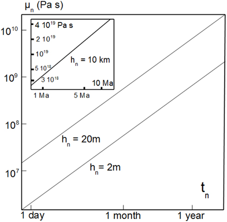
Figure 4. The two lines of similarity show that experiments on thick (hn = 10 km) spreading nappes (Merle, 1982) (the line of similarity of this experiment is shown in the insert) also simulate the strain within thin lava flows (hn = 20 m and hn = 2 m). Both horizontal and vertical axes have log scales. Explanation in the text.
The pi Theorem
Following Bertrand (1878), Waschi (1892) established the basis of the dimensional analysis in a well-known theorem. If a physical process involves n variables, or parameters a, there must be some kind of functional relationship between these variables, which can be written in implicit form as:
The actual form of this function may not be known but it describes the physics of the phenomenon. If p variables of these n variables are expressed in a fundamental unit (L, M, T, I, θ, N, J) then Equation (19) reduces to a simpler one in (n-p) variables:
where x1, x2, x3, … xn−p are monomial functions of a1, a2, … an.
In 1914, Buckingham extended this theorem, stating that there is an equivalent relation in terms of non-dimensional numbers. According to Buckingham (1914), if n variables of a physical process are expressed in p fundamental units, it is possible to re-arrange the n variables to form (n-p) independent dimensional numbers that describe the physics of the phenomenon. If the prototype is described by an equation similar to (19), having n variables expressed by p fundamental units, there is an equivalent relation to Equation (20) in terms of (n-p) independent dimensionless number π:
It is important to note that each dimensionless number must be independent and cannot be expressed as a product of another one. In relation to Buckingham's statement, Middleton and Wilcock (1994) write that “it is not obvious that this is true but it can be proved, though it is a curiosity of the history of dimensional analysis that many published “proofs” of this have subsequently been shown to be incomplete or invalid.”
The Waschi-Buckingham theorem, or simply the pi theorem, can be used to scale experiments. In Earth sciences, Tibaldi (1995) and Merle and Borgia (1996) were the first to scale experiments using it. The principle is to establish a list of dimensional numbers that describe the physical process. The experiment is said to be well scaled if each dimensional number in nature (πn) and model (πm) is of the same order of magnitude (πn≈ πm).
In practical terms, the experimenter has to: (1) Make a list of the n variables that are involved in the studied process; (2) Write the dimensions of these variables; (3) Determine the number p of fundamental units in which the n variables of the problem are expressed; and (4) Construct the (n-p) dimensional numbers used to describe the physics of the phenomenon. Unfortunately, the pi theorem does not guarantee that there is only one set of (n-p) dimensional numbers, so that various choices are possible when we reduce a list of dimensional variables to a set of dimensionless numbers. The challenge is then to determine the appropriate (n-p) dimensionless numbers.
Let us consider the n variables of the example (Figure 1) that are listed in Table 1 with their dimensions. The 10 variables (n = 10) are linked by a functional relation of that kind written in implicit form:
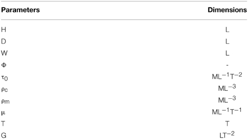
Table 1. The 10 principal parameters of the idealized example (Figure 1) are expressed in three dimensions only, which are length [L], mass [M], and time [T].
This function is not known. As in any purely mechanical problem, the 10 variables n are expressed through only three fundamental units (p = 3), which are length [L], mass [M], and time [T] (Table 1). So, we need seven dimensionless numbers (n − p = 7), which can be formed from the re-arrangement of the 10 variables, to scale this experiment. Then, instead of Equation (22), we can write a functional relation between 7 dimensionless numbers:
The first two dimensionless numbers may be the geometric ratio of the system:
These two dimensional numbers ensure that the model is geometrically similar to nature. Concerning the scaling of brittle material, the first parameter to be scaled is the angle of internal friction ϕ, which by definition is a dimensionless number. So, the third dimensional number is:
Due to the variety of shape of terrestrial volcanoes, π1 is not critical. For granular materials, the angle of repose (α) is considered as being equal to the angle of internal friction (ϕm), so that ϕm = α = atan [2 h/d]. This shows that, for granular materials, π3is not an independent dimensionless number as it can be expressed as a function of π1 (π3 = atan [2π1]). Moreover, once ϕm is close to 30/40°, this ensures a model slope of about 30/40°, similar to many volcanoes in nature, making π1 unnecessary.
The angle of internal friction (ϕ) controls the angle (θ) between the principal stress σ1 and the fault, as described by the formulae θ = π /4 – ϕ/2. According to Byerlee's law (Byerlee, 1978), most of the rocks in the upper part of the crust have ϕn ≈ 40° (τ = 0.85 σN). The analog granular materials used in this type of experiment generally have ϕm ≈ 35° (e.g., Merle et al., 2001; Holohan et al., 2008). Taking ϕn = 40° and ϕm = 35°, we obtain θn = 25° and θm = 27.5°, which is roughly the same. This shows that π3, together with π1, is not a dimensionless number which deserves much consideration either.
The cohesion (τ0) is the second parameter of the brittle material that has to be scaled. This can be done from Equation (6). The fourth dimensionless number is the ratio between the gravity stress and the cohesion:
This dimensionless number is a very important one in these types of experiments as it allows the cohesion to be scaled. Due to its high value in nature (105 to 107 Pa), cohesion has to be scaled down by several orders of magnitude in models. Small-scale experiments would not be feasible if analog materials with very low cohesions did not exist.
This ratio is nameless. Hubbert (1945) used a similar dimensionless number (i.e., the ratio between rock strength (σs) and gravity (ρ gh), π = σs/ρ gh) to demonstrate that very weak materials must be used in models to simulate geological structures. In recognition of Hubbert's considerable work on the theory of scale modeling in geology, I propose to call the ratio between gravity and cohesion the Hubbert number.
The fifth dimensionless number is the ratio between the density of the brittle cone and the density of the ductile magma:
The magma ascent may result from either buoyancy or overpressure, so this ratio is either higher or lower than 1. However, no matter which case is under consideration (buoyancy or overpressure), the density contrast in nature is low, so the π5 number is close to 1. Given the characteristics of analog materials at our disposal, this condition is always fulfilled in models. Consequently, this dimensionless number is not critical and does not deserve consideration.
The dependence between time and viscosity must be scaled. In the same way that Equation (6) allowed the determination of the fourth dimensionless number, the sixth dimensionless number may be formed by rearranging Equation (11):
This dimensionless number is the ratio between gravity and viscous forces (Fg/Fv). It has been proposed to call it the Ramberg number (Pollard and Fletcher, 2005). Together with the Hubbert number π4, this is a very important dimensionless number, which allows the viscosity in models to be scaled down.
In nature, there is a mechanical coupling between the brittle cone and the ductile magma. A dimensional number must verify that the resistance of the brittle cone with respect to the resistance of the ductile magma is the same in nature and in the model. This brittle/ductile coupling may be estimated by the ratio between the failure force in the brittle part and the viscous force in the ductile part.
The failure force per unit area is given by the Navier-Coulomb criterion of brittle failure τ = τ0 + σ tanϕ, where τ and σ are the shear and normal stresses acting at failure along the plane of rupture. Following reasonable approximations, the shear force τ per unit area may be expressed as a function of the principal stress σ1, which gives τ = 0.5 σ1tanϕ (see Appendix B). Considering the experiment in Figure 1, the main principal stress σ1 may be considered as being due to volcano loading (ρcgh) plus the viscous force (μ/t) of the ascending magma. Thus, the ratio between the failure force and the viscous force is:
As ρc≈ ρm, the π7 dimensionless number may be expressed as a product of the π6 Ramberg number:
or
According to the pi theorem, there is one dimensionless number too many. Using one renders the other unnecessary.
It might be important to ensure that inertia forces are negligible in the model, as in nature. This can be checked with the Reynolds number (Re), which is the ratio between inertia and viscous force (Fi/Fv).
It is not necessary for the Reynolds number to be of the same order of magnitude in the model and nature. It merely needs to be very low in both cases. In the example in Figure 1, π8 in nature and the model is about 5.4 10−9 and 7.7 10−8, respectively. The Reynolds number displays such small values that inertial forces are negligible with respect to viscous force. This is always true in this type of experiment, because the experiments last for too long a time span. In other words, calculating the Reynolds number to scale in such experiments is not necessary.
We have seen that only three dimensionless numbers (π2, π4, and π6) really need to be considered when scaling the experiment in Figure 1. Also, it must be noted that gm = gn (no centrifuge), so that g is a constant which has no influence when natural and model values of π4and π6 are compared. The gravitational acceleration g can thus be removed from these dimensionless numbers. Likewise, as ρcm ≈ ρcn and ρmm ≈ ρmn, the density values have little influence on the dimensional numbers. So, eliminating these two variables, we can write:
and:
Note that π′4 and π′6are not dimensionless. In the end, the physical process has only 6 variables (w, d, h, τ0, μ, t) that have to be taken into consideration and we only need three (n-p = 3) numbers (π2, π′4, π′6) to scale this experiment.
This example shows that choosing variables that play a role in the system is far from easy. Likewise, the significance of dimensional numbers must be discussed to determine which ones are really important. A proper application of the pi theorem to scale an experiment requires such a discussion. As mentioned before, more than (n-p) dimensional numbers may be formed from a set of variables. From Equation (22), eight have been proposed instead of seven, and others could have been discussed as well, like, for instance, the Froude, the Argand (England and McKenzie, 1982) or the Smolukowski (Ramberg, 1981) dimensionless numbers. The use of the pi theorem in scaling is a bit empirical, to say the least.
One thing is clear nevertheless. In experiments with brittle and ductile materials, the Hubbert and Ramberg numbers are the two fundamental dimensionless numbers which must be taken into consideration. Together with one or two geometric dimensionless numbers, they are enough to scale these types of experiments (Table 2).
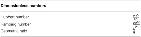
Table 2. The Hubbert and the Ramberg dimensionless numbers (plus one geometric ratio) are enough to scale the example in Figure 1.
The Use of Gelatin
Experimental studies on dyke formations need to intrude a fluid into a material, which fractures under the fluid pressure. Although granular materials can be used (see references in the section Types of experiments), gelatin is the classic analog material for this type of experiment (e.g., Hubbert and Willis, 1957; Hyndman and Alt, 1987; Takada, 1990; Heimpfel and Olson, 1994; Menand and Tait, 2002; Walter and Troll, 2003; Acocella and Tibaldi, 2005; Canon-Tapia and Merle, 2006; Menand et al., 2010). The rheology of gelatin is complex and it is doubtful that it can be considered as an analog for a volcanic edifice or the uppermost few hundred meters of the crust. This is because gelatin fails in tension, but not in shear, and is not appropriate for simulating faults within the crust (e.g., Galland et al., 2006).
Gelatin is a brittle visco-elastic solid but, on the time scale of the experiment, it behaves as a perfect elastic solid before failure. If we look at the elastic part of the gelatin's deformation, it is defined by a relation between normal stress (σ) and normal strain (e):
The proportionality coefficient E is the Young's modulus. As the Young's modulus has the dimension of a stress, it should be scaled down in models by a factor given by the stress ratio. The Young's modulus for gelatin is in the range of 103−104 Pa (e.g., Menand and Tait, 2002). In the example in Figure 1, σ* = 5 × 10⁻⁵. As the Young's modulus of rocks is about 1010 or 1011 Pa (e.g., Turcotte and Schubert, 1982), this yields a Young's modulus for the analog materials of about 5 × 10⁵ or 5 × 10⁶. The Young's modulus of the ideal analog material differs by at least one order of magnitude from that of the gelatin.
Looking at the rupture, the cohesion (τ0m) of the gelatin is about 103 Pa (Acocella and Tibaldi, 2005). Likewise the cohesion in the model must be scaled down by the same stress factor. Taking τ0n = 107 Pa, the cohesion in the model should be about 0.5 103 Pa, which is close to the cohesion of the gelatin. However, gelatin cannot simulate lower natural cohesions (106 Pa or 105 Pa). As it is rare that volcanoes are constituted of, unaltered, non-fractured, intact rocks, gelatin is a good analog only for some strong upper parts of the crust.
To overcome these difficulties, a more sophisticated approach has been put forward (e.g., Taisne and Tait, 2009; Kavanagh et al., 2013). The dyke propagation must be examined on a smaller length scale. The true length scale is the buoyancy length Lb, which is the length over which magma buoyancy driving ascent balances resistance from the fracture. This buoyancy length Lb is a function of the ratio between the fracture toughness (Kc) (i.e., the ability of a material containing a crack to resist fracture) and the buoyancy pressure gradient (Δρg) (see Equation 2 in Taisne and Tait, 2009). This allows the definition of the buoyancy length ratio:
If air is injected into gelatin, natural and experimental data make it possible to calculate the length ratio L*b, which is about 10−4 (Kavanagh et al., 2013). This is the same as in the example in Figure 1. The Young's modulus ratio E* may be calculated from the buoyancy length ratio L*b (Kavanagh et al., 2013):
where Ψ is the thickness of the dyke head at the opening of the dyke. E* varies from 10−6 –10−5. With a Young's modulus for rocks of about 1010–1011 Pa (e.g., Turcotte and Schubert, 1982), the appropriate analog material should exhibit a Young's modulus in the range of 104–106 Pa. Again, these values are a bit too high when compared with the average values of the Young's modulus for the gelatin, which are estimated to be in the range of 103–104 Pa (see Figure 2 in Menand and Tait, 2002).
However, the interest of this approach is to define a characteristic length scale for dyke formation which has nothing to do with the depth at which the deformation takes place. This specificity is not apparent in our idealized example (Figure 1) as this characteristic length scale is close to the length ratio of the example (L*b ≈ h*). If we consider a dyke forming at a depth of 20 km, this approach yields the same result for the Young's modulus needed in the experiments (i.e., 104–106 Pa).
Despite this difficulty in achieving perfect scaling using gelatin, experiments give interesting results on dyke propagation in nature. These discrepancies in the scaling have been noticed by several authors but they are probably minor in comparison with qualitative results from these experiments.
Pyroclastic Flows
Experiments on pyroclastic flows have to be examined separately because the physics mainly involves fluid dynamics and presents specific problems. Let us take the example of a dense, fluidized mixture of gas and particles, which may be the basal avalanche of a larger pyroclastic flow. The volume fraction of the particles is an important parameter making this flow a highly concentrated one, or non-turbulent if one refers to the terminology used for single-phase fluids. Due to the fluidization process, the flow may travel very far at an extremely rapid velocity. Clearly, the fluidization results from interstitial pore fluid pressure which counterbalances interparticle friction during motion.
Following Roche (2012) and considering a biphasic flow (gas and particles), the diameter (d) and the density (ρs) of the particle are two important parameters in the flow regime. The density (ρf) and dynamic viscosity (μ) of the interstitial fluid has to be considered, as well as the hydraulic permeability (k) and the diffusion coefficient (D) of the granular mixture, which also play an important role in controlling pore pressure generation and diffusion processes. Of course, the flow is also characterized by its thickness (h), length (L), and velocity (Uf). The gravitational acceleration (g) is the last parameter to take into consideration. In addition, there are two non-dimensional parameters: the particle volume fraction (εs) and the slope (α) along which the flow occurs. These two last parameters are chosen in the model to be equal to that in nature so they do not require further consideration. According to the pi theorem, and taking into consideration the 10 parameters (d,ρs,ρf,μ,k,D,h,L,Uf,g) minus three fundamental dimensions (length, mass, and time), seven dimensionless parameters should be enough to scale the model.
The useful dimensionless numbers in such experiments have been discussed in detail by Iverson (1997). Again, choosing the appropriate numbers is not easy. Roche (2012) uses seven dimensional numbers, which are the mass number (Ma), the Froude number (Fr), the Bagnold number (Ba), the Darcy number (Da), the Savage number (Sa) (Savage, 1984), the fluidization number (Fl), and the pore pressure number (Pr) (Iverson and Denlinger, 2001).
It is beyond the scope of this paper to define the role of all these dimensional numbers (see Iverson, 1997 for further details). The mass number reveals that air instead of water must be used as the fluid in experiments. High pore fluid pressure (high Darcy number and low Bagnold number) ensures an inviscid flow, which is supercritical, as confirmed by a Froude number higher than 1. At the end of the flow, when pore pressure becomes negligible, the low Savage number indicates that the flow propagates in a dry granular frictional regime (i.e., non-collisional). However, the high pore pressure number in models shows that pressure diffusion is faster than in the prototype, making the experimental flow run-out distance shorter than in nature. Thus, the thickness-to-length ratio of the deposit is not the same in nature and experiments. Despite this small discrepancy, the scaling is good enough to give many insights into the dynamics of pyroclastic flows (Roche, 2012). Again, the goal of modeling is not to duplicate a natural example but to explore the physical processes that take place during the flow.
Turbulent, dilute flows may also be studied experimentally. The scaling is achieved through several dimensionless numbers which are typically used in fluid dynamics, such as the Richardson, Froude, Stokes, and Reynolds numbers. These make it possible to ensure dynamic similarity between experiments and natural dilute density currents. An example of the discussion about these dimensional numbers may be found in Andrews and Manga (2012), which use talc powder turbulently suspended in air to simulate turbulent pyroclastic flows density currents.
Volcanic Explosions
To show the variety of volcanic systems that can be studied by scale modeling, the final example is of volcanic explosions. These could be triggered by phreatomagmatic eruptions, which form wide craters relative to their heights, resulting from excavation and collapse of surrounding rocks.
The problem is best tackled by the relation between the explosion energy (E) and both the crater diameter (d) and the explosion depth (h). It has been shown that the energy (E) is proportional to the third power of (d) and (h), which merely reveals that E is proportional to the volume [L3] of material disrupted. A simple general relation between energy (E) and crater diameter (d) has been calculated (Sato and Taniguchi, 1997):
Such a relationship is deduced from numerous artificial explosions, and is supposed to be applicable to natural phreatomagmatic craters. Scaled diameters (Sd) and scaled depths (Sh) can be defined from their relationships to energy. For instance, scaled diameter (Sd) is in the form:
Plotting the scaled depth versus the scaled diameter indicates that the main factor governing the crater diameter is the explosion depth (Goto et al., 2001). It also shows that, as the explosion depth (h) increases from zero to hmax, the diameter first enlarges then decreases for the deepest explosions (Goto et al., 2001). For a given crater diameter, this yields two solutions for the explosion depth, making the explosion depth difficult to assess in natural phreatomagmatic explosions from the simple measurement of diameter crater. However, small craters due to deep explosions are improbable in nature because this would require too much energy with respect to the strength of the host rocks.
To ensure good scaling, models must first fulfill the following condition: the diameter of the experimental crater versus the energy of the explosive charge must plot along (or nearly so) the line defined by Equation (38). This is probably not enough as this does not guarantee a ratio d/h similar to volcanic eruptions.
As noted by Goto et al. (2001), the rock strength is an important factor controlling the disruption of the host rock. Using the Hubbert number (Equation 26), it may be possible to determine the cohesion τ0m which would be appropriate for scaled experiments. The length ratio d* can vary from 10−3 to 10−2 in such experiments (see examples of natural and experimental data in Ross et al., 2013). The cohesion of the host rocks can vary from 107 Pa (i.e., strong granite) to 105 Pa (i.e., deeply altered and fractured volcanic rocks). This yields a range of cohesions τ0m for analog materials which varies from 0.5 105 Pa (dn = 1.5 × 10² m, dm = 1.5 m, ρ* = 0.5, τ0n = 107 Pa) to 0.5 × 10² Pa (dn = 1.5 × 10³ m, dm = 1.5 m, ρ* = 0.5, τ0n = 105 Pa).
Experiments using sand, pea gravel and crushed asphalt, such as those described in Valentine et al. (2012) and Ross et al. (2013), appear to be better scaled for large natural explosive craters (1500 m) with altered host rocks (τ0 = 105 Pa) than for small explosive craters (150 m) with resistant host rocks (τ0 = 107 Pa). It should be said, however, that analog materials in these experiments are moistened, which increases the cohesion τ0m to undetermined values.
Conclusion
Scale modeling has proved to be a useful tool in volcanology. A wide variety of volcanic systems have been studied over the last 20 years providing valuable insights into the understanding of these systems. The scaling procedure follows relatively simple rules that can be applied by anyone. Analog materials such as granular materials for brittle deformation or different kinds of silicone and oil for ductile deformation are easily available on the market. They are generally cheap and easy to handle. The experimental devices to set up in the laboratory are not expensive (if no centrifuge is involved) and can be done by the experimenter himself. For this reason, the cost/results ratio of this approach is excellent. If the experimenter is aware of the limitations of the method, scale modeling is “cheap and good” science.
Conflict of Interest Statement
The author declares that the research was conducted in the absence of any commercial or financial relationships that could be construed as a potential conflict of interest.
Acknowledgments
I thank Andrea Borgia for having drawn my attention to the pi theorem in 1995. This research was financed by the French Government Laboratory of Excellence initiative n°ANR-10-LABX-0006, the Région Auvergne and the European Regional Development Fund. This is Laboratory of Excellence ClerVolc contribution number 156. The two reviewers are thanked for their useful comments.
References
Abdelmalak, M. M., Mourgues, R., Galland, O., and Bureau, D. (2012). Fracture mode analysis and related surface deformation during dyke intrusion: results from 2D experimental modelling. Earth Planet. Sci. Lett. 359–360, 93–105. doi: 10.1016/j.epsl.2012.10.008
Absi, E. (1993). Pathologie Des Fondations et Des Ouvrages En Terre. Annales de L'institut Technique du Bâtiment et Des Travaux Publics, Série. Ouagadougou: Sols et Fondations.
Acocella, V., Cifelli, F., and Funiciello, R. (2000). Analogue models of collapse calderas and resurgent domes. J. Volcanol. Getherm. Res. 104, 81–96. doi: 10.1016/S0377-0273(00)00201-8
Acocella, V., Cifelli, F., and Funiciello, R. (2001). The control of overburden thickness on resurgent domes: insights from analogue models. J. Vocanol. Geotherm. Res. 111, 137–153. doi: 10.1016/S0377-0273(01)00224-4
Acocella, V., and Tibaldi, A. (2005). Dyke propagation driven by volcano collapse: a general model tested at Stomboli, Italy. Geophys. Res. Lett. 32, L08308. doi: 10.1029/2004GL022248
Andrews, J. A., and Manga, M. (2012). Experimental study of turbulence, sedimentation, and coignimbrite mass partitioning in dilute pyroclastic density currents. J. Volcanol. Geotherm. Res. 225–226, 30–44. doi: 10.1016/j.jvolgeores.2012.02.011
Barde-Cabusson, S., and Merle, O. (2007). From steep-slope volcano to flat caldera floor. Geophys. Res. Lett. 34, L10305. doi: 10.1029/2007gl029784
Barenblatt, G. I. (1996). Scaling, Self-Similarity, and Intermediate Asymptotics. Cambridge: Cambridge University Press. doi: 10.1017/cbo9781107050242
Branquet, Y., and van Wyk de Vries, B. (2001). Effects of volcanic loading on regional compressive structures: new insights from natural examples and analogue modelling. Comptes Rendus de L'académie Des Sci. 333, 455–461. doi: 10.1016/S1251-8050(01)01660-3
Brothelande, E., and Merle, O. (2015). Estimation of magma depth in resurgent domes: an experimental approach. Earth Planet. Sci. Lett. 412, 143–151. doi: 10.1016/j.epsl.2014.12.011
Brun, J. P. (1999). Narrow rifts versus wide rifts: inferences for the mechanics of rifting from laboratory experiments. Philos. Trans. R. Soc. Lond. A 357, 695–712. doi: 10.1098/rsta.1999.0349
Brun, J. P., and Merle, O. (1985). Strain pattern in models of spreading-gliding nappes. Tectonics 4, 705-719. doi: 10.1029/TC004i007p00705
Bucher, W. H. (1956). Role of gravity in orogenesis. Bull. Geol. Soc. Am. 67, 1295-1318. doi: 10.1130/0016-7606(1956)67[1295:rogio]2.0.co;2
Buckingham, E. (1914). On physically similar system: illustration of the use of dimensional analysis. Phys. Rev. 4, 345–376. doi: 10.1103/PhysRev.4.345
Buisson, C., and Merle, O. (2002). Experiments on internal strain in lava dome cross-sections. Bull. Volcanol. 64, 363–371. doi: 10.1007/s00445-002-0213-6
Buisson, C., and Merle, O. (2005). “Influence of the crustal thickness on dome destabilization,” in Kinematics and Dynamics of Lava Flows: Geological Society of America Special Paper396, eds M. Manga and G. Ventura (Boulder, CO: Geological Society of America, Inc.), 181–188.
Byrne, P. K., Holohan, E. P., Kervyn, M., van Wyk de Vries, B., Troll, V. R., and Murray, J. B. (2013). Sagging-spreading continuum of large volcano structure. Geology 41, 339–342. doi: 10.1130/G33990.1
Cadell, H. M. (1889). Experimental researches in moutain building. Trans. R. Soc. Edimbourg (Pt. 1), 35, 339–343.
Canon-Tapia, E., and Merle, O. (2006). Dyke nucleation and early growth from pressurized magma chambers: insights from analogue models. J. Volcanol. Geotherm. Res. 158, 207–220. doi: 10.1016/j.jvolgeores.2006.05.003
Cecchi, E., van Wyk de Vries, B., and Lavest, J. M. (2005). Flank spreading and collapse of weak-cored volcanoes. Bull. Volcanol. 67, 72–91. doi: 10.1007/s00445-004-0369-3
Cloos, E. (1955). Experimental analysis of fracture patterns. Geol. Soc. Am. Bull. 66, 241–256. doi: 10.1130/0016-7606(1955)66[241:EAOFP]2.0.CO;2
Cobbold, P. R., and Castro, L. (1999). Fluid pressure and effective stress in sandbox modelling. Tectonophysics 301, 1–19. doi: 10.1016/S0040-1951(98)00215-7
Daubrée, A. (1879). Expériences sur la deformation des fossiles en relation avec la schistosité des roches. Etudes Synthétiques de Géologie Expérimentale. Paris: Dunod.
Davy, P., and Cobbold, P. R. (1988). Indentation tectonics in nature and experiment. I. Experiments scaled for gravity. Bull. Geol. Inst. Uppsala 14, 129–141.
Delcamp, A., van Wyk de Vries, B., and James, M. (2008). The influence of edifice slope and substrata on volcano spreading. J. Volcanol. Geotherm. Res. 177, 925–943. doi: 10.1016/j.jvolgeores.2008.07.014
Dixon, J. M., and Summers, D. G. (1985). Recent development in centrifuge modelling of tectonic processes: equipment, model construction techniques and rheology of model materials. J. Struct. Geol. Lond. 134, 201–213.
Donnadieu, F., and Merle, O. (1998). Experiments on the indentation process during cryptodome intrusion: new insights into Mt St Helens deformation. Geology 26, 79–82.
Eichelberger, J. C., and Hayes, D. B. (1982). Magmatic models for the Mount St Helens blast of May 18. J. Geophys. Res. 87, 7727–7738. doi: 10.1029/JB087iB09p07727
England, P. C., and McKenzie, D. (1982). A thin viscous sheet model for continental deformation. Geophys. J. R. Astron. Soc. 70, 295–321. doi: 10.1111/j.1365-246X.1982.tb04969.x
Galerne, C., Galland, O., Neumann, E. R., and Planke, S. (2011). 3D relationships between sills and their feeders: evidence from the golden valley sill complex (Karoo basin) and experimental modelling. J. Volcanol. Geotherm. Res. 202, 189–199. doi: 10.1016/j.jvolgeores.2011.02.006
Galland, O. (2012). Experimental modelling of ground deformation associated with shallow magma intrusions. Earth Planet. Sci. Lett. 317/318, 145–156. doi: 10.1016/j.epsl.2011.10.017
Galland, O., Cobbold, P. R., de Bremond d'Ars, J., and Hallot, E. (2007). Rise and emplacement of magma during horizontal shortening of the brittle crust: insights from experimental modelling. J. Geophys. Res. 112, B06402. doi: 10.1029/2006jb004604
Galland, O., Cobbold, P. R., Hallot, E., and de Bremond d'Ars, J. (2006). Use of vegetable oil and silica powder for scale modelling of magmatic intrusion in a deforming brittle crust. Earth Planet. Sci. Lett. 243, 786–804. doi: 10.1016/j.epsl.2006.01.014
Galland, O., de Bremond d'Ars, J., Cobbold, P. R., and Hallot, E. (2003). Physical models of magmatic intrusion during thrusting. Terra Nova 15, 405–409. doi: 10.1046/j.1365-3121.2003.00512.x
Galland, O., Planke, S., Neumann, E. R., and Malthe-Sorenssen, A. (2009). Experimental modelling of shallow magma emplacement: application to saucer-shaped intrusions. Earth Planet. Lett. 277, 373–383. doi: 10.1016/j.epsl.2008.11.003
Geyer, A., Folch, A., and Marti, J. (2006). Relationship between caldera collapse and magma chamber withdrawal: an experimental approach. J. Volcanol. Geotherm. Res. 157, 375–386. doi: 10.1016/j.jvolgeores.2006.05.001
Girard, G., and van Wyk de Vries, B. (2005). The Managua graben and Las Sierras-Masaya volcanic complex (Nicaragua); pull-apart localization by an intrusive complex: results from analogue modelling. J. Volcanol. Geotherm. Res. 144, 37–57. doi: 10.1016/j.jvolgeores.2004.11.016
Goto, A., Tanigushi, H., Yoshida, M., Tsukasa, O., and Oshima, H. (2001). Effects of explosion energy and depth to the formation of blast wave and craters: field explosion experiments for the understanding of volcanic explosion. Geophys. Res. Lett. 28, 4287–4290. doi: 10.1029/2001GL013213
Hall, J. (1815). On the vertical position and convolutions of certain strata, and their relation with granite. Trans. R. Soc. Edinburgh 7, 85–86. doi: 10.1017/S0080456800019268
Handin, J. (1966). “Strength and ductility,” in Handbook of Physical Constants, Vol. 97, ed S. P. Clark, (Boulder, CO: Geol. Soc. Am. Memoir) 223. doi: 10.1130/MEM97-p223
Heimpfel, M., and Olson, P. (1994). “Buoyancy-driven fracture and magma transport through the lithosphere: models and experiments,” in Magmatic Systems, ed M. P. Ryan (San Diego, CA: Academic Press), 223–240.
Holohan, E. P., Troll, V. P., Walter, T. R., Münn, S., McDonnel, S., and Shipton, Z. K. (2005). Elliptical calderas in active tectonic settings: an experimental approach. J. Volcanol. Geotherm. Res. 144, 119–136. doi: 10.1016/j.jvolgeores.2004.11.020
Holohan, E. P., van Wyk de Vries, B., and Troll, V. R. (2008). Analogue models of caldera collapse in strike-slip tectonic regimes. Bull. Volcanol. 70, 773–796. doi: 10.1007/s00445-007-0166-x
Hoshino, K. H., Koide, K., Inami, S., Iwamura, S., and Mitsui, S. (1972). Mechanical properties of Japanese tertiary sedimentary rocks under high confining pressures. Geol. Surv. Jpn. Rep. 244.
Hubbert, M. K. (1937). Theory of scale models as applied to the study of geologic structures. Geol Soc. Am. Bull. 48, 1459-1520.
Hubbert, M. K., and Rubey, W. W. (1959). Role of fluid pressure in mechanics of overthrust faulting, I. mechanics of fluid-filled porous solids and its application to overthrust faulting. Geol. Soc. Am. Bull. 70, 115-166. doi: 10.1130/0016-7606(1959)70[115:rofpim]2.0.co;2
Hubbert, M. K., and Willis, D. G. (1957). “Mechanics of hydraulic fracturing,” in Structural Geology, ed M. K. Hubbert (New York, NY: Hafner Publishing Company), 175–190.
Hyndman, D. W., and Alt, D. (1987). Radial dikes, laccoliths, and gelatin models. J. Geol. 95, 763–774. doi: 10.1086/629176
Iverson, R. M. (1997). The physics of debris flows. Rev. Geophys. 35, 245–296. doi: 10.1029/97RG00426
Iverson, R. M., and Denlinger, R. P. (2001). Flow of variably fluidized granular masses across three-dimensional terrain 1. Coulomb mixture theory. J. Geophys. Res. 106, 537–552. doi: 10.1029/2000JB900329
Jaeger, J. C., and Cook, N. G. W. (1971). Fundamental of Rocks Mechanics. New York, NY: Chapman and Hall.
Kavanagh, J. L., Menand, T., and Daniels, K. A. (2013). Gelatine as a crustal analogue: determining elastic properties for modelling magmatic intrusions. Tectonophysics 582, 101–111. doi: 10.1016/j.tecto.2012.09.032
Kervyn, M., van Wyk de Vries, B., Walter, T. R., Njome, M. S., Suh, C. E., and Ernst, G. G. J. (2014). Directional flank spreading at mount Cameroun volcano: evidence from analogue modeling. J. Geophys. Res. 119, 7542–7563. doi: 10.1002/2014JB011330
Koenigsberger, J. and Morath, O. (1913). Theoretische Grundlagen der experimentellen Tektonik. Z. Deut. Geol. Gessell. 65, 65–86.
Komuro, H. (1987). Experiments on cauldron formation: a polygonal cauldron and ring fractures. J. Volcanol. Geotherm. Res. 31, 139–149. doi: 10.1016/0377-0273(87)90011-4
Krantz, R. W., (1991). Measurements of friction coefficients and cohesion for faulting and fault reactivation in laboratory models using sand and sand mixtures. Tectonophysics 188, 203–207. doi: 10.1016/0040-1951(91)90323-K
Lagmay, A. M. F., van Wyk de Vries, B., Kerle, N., and Pyle, D. M. (2000). Vocano instability induced by strike-slip faulting. Bull. Volcanol. 62, 331–346. doi: 10.1007/s004450000103
Le Corvec, N., and Walter, T. R. (2009). Volcano spreading and fault interaction influenced by rift zone intrusions: insights from analogue experiments analyzed with digital image correlation technique. J. Volcanol. Geotherm. Res. 183, 170–182. doi: 10.1016/j.jvolgeores.2009.02.006
Le Corvec, N., Walter, T. R., Ruch, J., Bonforte, A., and Puglisi, G. (2014). Experimental study of the interplay between magmatic rift intrusion and flank instability with application to the 2001 Mount Etna eruption. J. Geophys. Res. 119, 5356–5368. doi: 10.1002/2014JB011224
Lescinsky, D., and Merle, O. (2005). Extensional and compressional strain in lava flows and the formation of fractures in surface crust. Kinemat. Dyn. Lava Flows 396, 161–177.
Lohrmann, J., Kukowski, N., Adam, J., and Oncken, O. (2003). The impact on analogue material properties on the geometry, kinematics and dynamics of convergent sand wedges. J. Struct. Geol. 25, 1691–1711. doi: 10.1016/S0191-8141(03)00005-1
Marotta, E., and de Vita, S. (2014). The role of pre-existing tectonic structures and magma chamber shape on the geometry of resurgent blocks, analogue models. J. Volcanol. Geotherm. Res. 272, 23–38. doi: 10.1016/j.jvolgeores.2013.12.005
Marti, J., Ablay, G. J., Redshaw, L. T., and Sparks, R. S. J. (1994). Experimental studies on collapse calderas. J. Geol. Soc. Lond. 151, 919–929. doi: 10.1144/gsjgs.151.6.0919
Mathieu, L., van Wyk de Vries, B., Holohan, E., and Troll, V. (2008). Dykes, cups, saucers and sills: analogue experiments on magma intrusion into brittle rocks. Earth Planet. Sci. Lett. 271, 1–13. doi: 10.1016/j.epsl.2008.02.020
Menand, T., Daniels, K. A., and Benghiat, P. (2010). Dyke propagation and sill formation in a compressive tectonic environment. J. Geophys. Res. 115, B08201. doi: 10.1029/2009jb006791
Menand, T., and Tait, S. R. (2002). The propagation of a buoyant liquid-filled fissure from a source under constant pressure: an experimental approach. J. Geophys. Res. 107, 2306. doi: 10.1029/2001jb000589
Merle, O. (1982). Cinématique et déformation de la nappe du Parpaillon, Alpes Occidentales. Ph.D. thesis, Rennes, 147p.
Merle, O. (1998). Internal strain within lava flows from analogue modelling. J. Volcanol. Geotherm. Res. 81, 189–206. doi: 10.1016/S0377-0273(98)00009-2
Merle, O., Barde-Cabusson, S., Maury, R. C., Legendre, C., Guille, G., and Blais, S. (2006). Volcano core collapse triggered by regional faulting. J. Volcanol. Geotherm. Res. 158, 269–280. doi: 10.1016/j.jvolgeores.2006.06.002
Merle, O., and Borgia, A. (1996). Scaled experiments on volcanic spreading. J. Geophys. Res. 101, 13805–13817. doi: 10.1029/95JB03736
Merle, O., and Lénat, J.-F. (2003). Hybrid collapse mechanism at Piton de la Fournaise (Reunion Island, Indian Ocean). J. Geophys. Res. 108, 2166–2176. doi: 10.1029/2002JB002014
Merle, O., van Wyk de Vries, B., and Barde-Cabusson, S. (2010). Hydrothermal calderas. Bull. Volcanol. 72, 131–147. doi: 10.1007/s00445-009-0314-6
Merle, O., and Vendeville, B. (1995). Experimental modelling of thin-skinned shortening around magmatic intrusions. Bull. Volcanol. 57, 33–43.
Merle, O., Vidal, N., and Van Wyk de Vries, B. (2001). Experiments on vertical basement fault reactivations below volcanoes. J. Geophys. Res. 106, 2153–2162. doi: 10.1029/2000JB900352
Middleton, G. V., and Wilcock, P. R. (1994). Mechanics in the Earth and Environmental Sciences. Cambridge: Cambridge University Press.
Mourgues, R., and Cobbold, P. R. (2003). Some tectonic consequences of fluid overpressures and seepage forces as demonstrated by sandbox modeling. Tectonophysics 376, 75–97. doi: 10.1016/S0040-1951(03)00348-2
Murase, T., McBirney, A. R., and Melson, W. G. (1985). Viscosity of the dome of Mount St Helens. J. Volcanol. Geotherm. Res. 24, 193–204. doi: 10.1016/0377-0273(85)90033-2
Nicolas, A., and Ildefonse, B. (1996). Flow mechanics and viscosity in basaltic magma chambers. Geophys. Res. Lett. 23, 2013–2016. doi: 10.1029/96GL02073
Norini, G., and Acocella, V. (2011). Analogue modeling of flank instability at Mount Etna: understanding the driving factors. J. Geophys. Res. 116, B07206. doi: 10.1029/2011jb008216
Norini, G., and Lagmay, A. M. F. (2005). Deformed symmetrical volcanoes. Geology 33, 605–608. doi: 10.1130/G21565.1
Odonne, F., Ménard, I., Massonnat, G. J., and Rolando, J.-P. (1999). Abnormal reverse faulting above a depleting reservoir. Geology 27, 111–114.
Oehler, J. F., van Wyk de Vries, B., and Labazuy, P. (2005). Landslides and spreading of oceanic hot-spot and arc shield volcanoes on low strength layers; an analogue modelling approach. J. Volcanol. Geotherm. Res. 144, 169–189. doi: 10.1016/j.jvolgeores.2004.11.023
Panien, M., Schreurs, G., and Pfiffner, A. (2006). Mechanical behavior of granular materials used in analogue modelling: insights from grain characterization, ring-shear tests and analogue experiments. J. Struct. Geol. 28, 1710–1724. doi: 10.1016/j.jsg.2006.05.004
Platz, T., Munn, S., Walter, T. R., Procter, J. N., Mc Guire, P. C., Dumke, A., et al. (2011). Vertical and lateral collapse of Tharsis Tholus, Mars. Earth Planet. Sci. Lett. 305, 445–455. doi: 10.1016/j.epsl.2011.03.012
Pollard, D. D., and Fletcher, R. C. (2005). Fundamental of Structural Geology. Cambridge: Cambridge University Press.
Price, N. J. (1966). Fault and Joint Development in Brittle and Semi-Brittle Rock. Oxford: Pergamon Press.
Ramberg, H. (1971). Dynamic models simulating rift valleys and continental drift. Lithos 4, 259–276. doi: 10.1016/0024-4937(71)90006-5
Roche, O. (2012). Depositional processes and gas pore pressure in pyroclastic flows: an experimental perspective. Bull. Volcanol. 74, 1807–1820. doi: 10.1007/s00445-012-0639-4
Roche, O., Druitt, T. H., and Merle, O. (2000). Experimental study of caldera formation. J. Geophys. Res. 105, 395–416. doi: 10.1029/1999JB900298
Roman-Bierdel, T., Gapais, D., and Brun, J. P. (1995). Analogue models of laccolith formation. J. Struct. Geol. 17, 1337–1346. doi: 10.1016/0191-8141(95)00012-3
Ross, P.-S., White, J. D. L., Valentine, G. A., Taddeucci, J., Sonder, I., and Andrews, R. G. (2013). Experimental birth of a maar-diatreme volcano. J. Volcanol. Geotherm. Res. 260, 1–12. doi: 10.1016/j.jvolgeores.2013.05.005
Sato, H., and Taniguchi, H. (1997). Relationship between crater size and ejecta volume of recent magmatic and phreato-magmatic eruptions: implication for energy partitioning. Geophys. Res. Lett. 24, 205–208. doi: 10.1029/96GL04004
Savage, S. B. (1984). The mechanics of rapid granular flows. Adv. Appl. Mech. 24, 289–366. doi: 10.1016/s0065-2156(08)70047-4
Schellart, W. P. (2000). Shear test results for cohesion and friction coefficients for different granular materials: scaling implications for their usage in analogue modelling. Tectonophysics 324, 1–16. doi: 10.1016/S0040-1951(00)00111-6
Schultz, R. A. (1996). Relative scale and the strength and deformability of rock masses. J. Struct. Geol. 18, 1139–1149. doi: 10.1016/0191-8141(96)00045-4
Shaw, H. R. (1972). Viscosities of magmatic silicate liquids: an empirical method of prediction. Am. J. Sci. 272, 870–893. doi: 10.2475/ajs.272.9.870
Sollas, W. J. (1906). - Recumbent folds produced as a result of flow. Q. J. Geol. Soc. Lond. 62, 716-721.
Taisne, B., and Tait, S. (2009). Eruption versus intrusion? Arrest of propagation of constant volume, buoyant, liquid-filled cracks in an elastic, brittle host. J. Geophys. Res. 114. doi: 10.1029/2009JB006297
Takada, A. (1990). Experimental study on propagation of liquid-filled crack in gelatin: shape and velocity in hydrostatic stress condition. J. Geophys. Res. 95, 8471–8481. doi: 10.1029/JB095iB06p08471
Tibaldi, A. (1995). Morphology of pyroclastic cones and tectonics. J. Geophys. Res. 100, 24521–24535. doi: 10.1029/95JB02250
Tibaldi, A. (2008). Contractional tectonics and magma paths in volcanoes. J. Volcanol. Geotherm. Res. 176, 291–301. doi: 10.1016/j.jvolgeores.2008.04.008
Tibaldi, A., Bistachi, L., Pasquarè F. A., and Vezzoli, L. (2006). Extensional tectonics and volcano lateral collapses: insights from Ollague volcano (Chile-Bolivia) and analogue modelling. Terra Nova 18, 282–289. doi: 10.1111/j.1365-3121.2006.00691.x
Troll, V. R., Walter, T. R., and Schmincke, H. U. (2002). Cyclic caldera collapse piston or piecemeal subsidence? Field and experimental data. Geology 30, 135–138. doi: 10.1130/0091-7613(2002)030<0135:CCCPOP>2.0.CO;2
Turcotte, D. L., and Schubert, G. (1982). Applications of Continuum Physics to Geological Problems. New York, NY: John Wiley & sons ed.
Valentine, G. A., White, J. D. L., Simon, P.-S., Amin, J., Taddeucci, J., Sonder, I., et al. (2012). Experimental craters formed by single and multiple buried explosions and implications for volcanic craters with emphasis on maars. Geophys. Res. Lett. 39, 20. doi: 10.1029/2012GL053716
Van Wyk de Vries, B., Kerle, N., and Petley, D. (2000). Sector collapse forming at casita volcano, Nicaragua. Geology 28, 167–170. doi: 10.1130/0091-7613(2000)28<167:SCFACV>2.0.CO;2
van Wyk de Vries, B., and Merle, O. (1996). The effect of volcanic construct on rift fault patterns. Geology 24, 643–646.
van Wyk de Vries, B., and Merle, O. (1998). Extension induced by volcanic loading in strike-slip fault zones. Geology 26, 983–986.
Walter, T. R. (2003). Buttressing and fractional spreading of Tenerife, an experimental approach on the formation of rift zones. J. Geophys. Res. 30, 1296. doi: 10.1029/2002GL016610
Walter, T. R., Klugel, A., and Munn, S. (2006). Gravitational spreading and formation of new rift zones on overlapping volcanoes. Terra Nova 18, 26–33. doi: 10.1111/j.1365-3121.2005.00656.x
Walter, T. R., and Troll, V. R. (2001). Formation of periphery faults: an experimental study. Bull. Volcanol. 63, 191–203. doi: 10.1007/s004450100135
Walter, T. R., and Troll, V. R. (2003). Experiments on rift zone evolution in unstable volcanic edifices. J. Volcanol. Geotherm. Res. 127, 107–120. doi: 10.1016/S0377-0273(03)00181-1
Weijermars, R. (1986). Flow behaviour and physical chemistry of bouncing putties and related polymers in view of tectonic laboratory applications. Tectonophysics 124, 325–358.
Willis, B. (1891/1892). The Mechanics of Appalachian Structure. 13th Annual Report. U.S. Geol. Surv., 217–281.
Appendix A
The cohesion of the analog material may be calculated from the highest vertical wall which remains stable without failure. As known from civil engineering studies (e.g., Philipponat and Hubert, 1997), the upper part of the vertical wall is in tension, whereas the lower part is in compression (Figure A1). Increasing H leads to failure which occurs at H/2, a singular point where the least stress axis σ3 is nullified. From the Mohr–Coulomb theory, it is known that the two principal stress axes σ1 (=ρgh) and σ3 are linked by the following equation when failure occurs:
Where
and
with τ0 and ϕ the cohesion and the angle of friction of the material, respectively [see Equations (7–9) in (Hubbert and Rubey, 1959)].
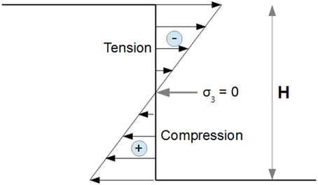
Figure A1. The σ3 distribution as a function of H along a vertical wall (after Philipponat and Hubert, 1997).
At the point H/2 where σ3 is nullified, Equation (A1) simplifies to:
from which τ0 can be extracted (Merle et al., 2001):
Appendix B
The failure force per unit area is given by the Navier-Coulomb criterion of brittle failure:
where τ and σN are the shear and normal stresses acting at failure along the plane of rupture.
The relation between σN and the main principal stresses σ1 and σ3 is given by the classical formula of the Mohr circle (see Equation (6) in Price, 1966):
where θ is the angle between the rupture plane and σ1. The angle θ is close to 30° for most rocks, making cos 2θ = 0.5. In a volcanic edifice where rocks are altered and fractured, the cohesion τ0 (106/105 Pa) is one or two orders of magnitude less than for intact rocks (107 Pa). Compared to the principal stresses σ1 and σ3 needed to fracture the rocks (2.8 × 10⁷ Pa in an edifice of 1000 m high), the cohesion can be considered as being negligible. From Equations (A1–A3), it follows (ϕ = 30°):
Then, solving equation (A7) for σ1, yields:
and, from Equation (A6), the failure force per unit area is:
Keywords: volcanology, scaling, experiments, scaled-models, scale factors, pi theorem, Volcanology
Citation: Merle O (2015) The scaling of experiments on volcanic systems. Front. Earth Sci. 3:26. doi: 10.3389/feart.2015.00026
Received: 12 March 2015; Accepted: 24 May 2015;
Published: 12 June 2015.
Edited by:
Adelina Geyer, Institute of Earth Sciences Jaume Almera (ICTJA-CSIC), SpainReviewed by:
Alvaro Marquez, Universidad Rey Juan Carlos, SpainThomas R. Walter, GFZ German Research Centre for Geosciences, Germany
Copyright © 2015 Merle. This is an open-access article distributed under the terms of the Creative Commons Attribution License (CC BY). The use, distribution or reproduction in other forums is permitted, provided the original author(s) or licensor are credited and that the original publication in this journal is cited, in accordance with accepted academic practice. No use, distribution or reproduction is permitted which does not comply with these terms.
*Correspondence: Olivier Merle, Laboratoire Magmas et Volcans, Université Blaise Pascal - Centre National de la Recherche Scientifique - IRD, OPGC, 5 rue Kessler, 63038 Clermont Ferrand, France, o.merle@opgc.fr