Mitigation of model error effects in neural network-based structural damage detection

1 Introduction

The knowledge of the actual structural health condition of the built heritage is a key aspect for its preservation and maintenance. Several factors, such as ageing, seismic events, exposure to adverse environmental conditions and so on, can cause damage to a structure. The lack of knowledge or the underestimation of the structural damage may lead to a progressive or an abrupt decline of the structural health that may prevent its serviceability or cause collapses. The monitoring of the structural health over time enables to recognize critical situations and carry out effective countermeasures to prevent collapses. The structural health monitoring (SHM) is that branch of research aimed at developing different solutions, in terms of sensor equipment (Savoia et al., 2014; Castagnetti et al., 2019) and procedures, to detect changes and abnormalities in the structural response to different sources of excitation (Bassoli et al., 2015; 2018a; Vincenzi et al., 2019). Typical SHM systems are designed to investigate the dynamic behaviour of a structure (Bassoli et al., 2018b), being it directly related to the global structural integrity. The dynamic properties of a structure, indeed, depend on its stiffness, that typically reduces when damage occurs. Despite the possibility of artificially excite a structure, most common and less invasive monitoring approaches rely on the measurement of the vibration response to unknown environmental source of excitation and the subsequent identification of the structural dynamic features (Brincker et al., 2001; Rainieri and Fabbrocino, 2010). Modal properties are often assumed as representative features of the structural health state, since they can provide information about both the global (e.g. natural frequencies) and the local (e.g. mode shapes or modal curvatures) structural behaviour (Doebling et al., 1996; Sohn et al., 2002; Comanducci et al., 2016).

Damage detection methods are commonly divided in two main groups: model-based and data-driven methods. The first group directly adopts numerical models to describe the structure and identify, localize and quantify damage (Hosamo et al., 2022). The stiffness reduction of an element or a group of elements, representing the damage severity, can be detected by repeating the model calibration for different measurement epochs (Friswell, 2008; Alves et al., 2020; Rosati et al., 2022). Model updating allows to reduce as much as possible the discrepancy between the experimental observations and the same quantities predicted by the numerical model by adjusting suitable model parameters (Ponsi et al., 2021; 2022). This discrepancy is expressed by means of specific functions that, in the case of modal properties, are related to frequency and mode shape residuals. The efficiency and accuracy of the damage detection procedure strongly depend on several aspects, such as the quality and the quantity of available experimental observations, the model parametrization, the definition of the optimization problem and the algorithm employed for its resolution (Mthembu et al., 2011; Reynders, 2012; Bianconi et al., 2020; Standoli et al., 2021). The quantification of the uncertainty affecting the updated parameters can be performed with a Bayesian approach (Monchetti et al., 2022), thus allowing the detection to be performed in stochastic terms (Bartoli et al., 2019).

Model based damage detection methods are usually time-consuming and do not enable the real-time identification of a damaged condition. On the contrary, data-driven methods are based on the extraction of damage-sensitive features directly from the measured response, without needing to develop and calibrate a structural model. As a consequence, the computational effort required by these methods is strongly reduced and a real-time identification of the structure condition can be carried out. In this context, the choice of the damage-sensitive features plays a fundamental role.

Early data-driven methods adopted natural frequencies and mode shapes as damage-sensitive features (Doebling et al., 1996). However, the low sensitivity to local damage and the high sensitivity to environmental conditions of natural frequencies and the uncertainty in the identification of mode shapes make the use of these parameters not particularly suited for damage identification purposes. Trying to overcome these limitations, other damage-sensitive features related to modal properties have been proposed in literature, such as the mode shape curvature (Pandey et al., 1991), the modal strain energy and the modal flexibility (Pandey and Biswas, 1994). However, being these indices related to mode shapes, their computation magnifies the effect of noise and errors and they require a dense sensor network. In contrast to modal data, damage detection methods based on frequency response functions (FRF) (Limongelli, 2010), operational deflection shapes (ODF) and transmissibility (Ribeiro et al., 2000) have been proposed. The main drawbacks related to FRF application involve the choice of the optimum frequency range and the need to measure excitation force and structural response simultaneously.

Studies and results presented in literature highlight the necessity to develop statistical models for feature discrimination, since the effect of noise or other external factors on the selected features may lead to false alarms or mask damage effects (Sohn et al., 2002). Machine learning (ML) techniques represent an effective solution to this problem since they are capable of working with uncertain and noise-corrupted data (Khan and Yairi, 2018; Klepac and Subgranon, 2022). The application of these techniques to the field of damage detection is quite recent, but a vast amount of works have been produced. The widespread adoption of ML techniques is due to the great computational development in recent years that enables collecting, handling and elaborating a huge amount of data. In this context, damage detection procedure is addressed as a pattern recognition problem, whose main phases are data acquisition, feature extraction and classification. The last task is usually accomplished by ML classifiers, among which artificial neural networks (ANN) are the most diffused (Luleci et al., 2022). Review works that aim at the classification of ML-based damage detection techniques are those of Avci et al. (2021) and Hou and Xia (2021). ML damage detection methods can be distinguished depending on the employed feature extraction technique (Avci et al., 2021). Parametric methods use structural dynamic parameters to determine the presence, location and severity of damage. These parameters are physical parameters like modal frequencies, masses, dampings and mode shapes. In this case, modal identification techniques are employed for feature extraction. Some examples of the parametric ML methods for damage detection that can be found in literature are Lam and Ng (2008), Bakhary et al. (2010) and Betti et al. (2015). On the other hand, non-parametric methods detect damage directly from the acquired accelerations by means of statistical tools. Time series modelling and signal processing techniques are employed to extract damage sensitive features that are then provided to a classifier (Figueiredo et al., 2010; Osama and Onur, 2016). Numerical models are not directly involved in the identification of a damaged state with data-driven methods, but they may be employed to create data related to damaged scenarios that cannot be reproduced in a real situation. Several methods, indeed, have been developed starting from information generated by models, like the integrated use of spatial Fourier analysis and artificial neural networks of Pawar et al. (2006) or the two-phase detection method of Yuen and Lam (2006).

This paper proposes a complete procedure for damage detection that exploits ML techniques, in particular artificial neural networks. In the context of civil engineering applications, it is possible to measure a large amount of data related to the undamaged condition of a structure, while it is basically impossible to measure the structural response in damaged conditions. This means that experimental data relative to different damage scenarios required to train and test the neural network cannot be available. This is the reason why FE models are widely employed to generate data relative to different damage scenarios. To this purpose, a FE model of the structure should be built and calibrated with reference to the experimental measurements acquired from the monitoring system installed on the structure. However, even if the FE model is accurately calibrated, experimental results and model predictions will never exactly match and their difference represents the model error. Being the neural network tested and trained with respect to the data generated from the numerical model, the model error can significantly compromise the effectiveness of the damage detection procedure. Taking into account and mitigating the effect of the model error is the key aspect of the proposed procedure. To show the effectiveness of the presented procedure and its suitability to different applications, both a numerical and a real case study are presented. The numerical case study is a railway bridge for which real experimental data are replaced by pseudo-experimental data generated by a numerical model. The real case study is the widely adopted ASCE benchmark structure described in Dyke et al. (2001, 2003), namely a steel braced frame. Although in the first case the proposed procedure is presented with simulated data only, we have accounted for critical aspects to ensure that the results are representative of real situations, namely the stochastic modelling of measurement errors and the use of two different numerical models to account for the model error. In the paper, the response of an accurate model (called the “reference” model) is considered in place of the experimental data while a simpler model (called the “support” model) is used to train the network. This allows us to account for the fact that simulated data never exactly reproduce the reference results even if the numerical model is well calibrated with respect to the experimental data. Moreover, different networks are studied, each of one taking as input modal properties that have been elaborated in different ways. A proposal is presented in order to prevent the misclassification of the undamaged condition due to the model error. In particular, the residual error obtained at the end of the calibration procedure is added to the modal properties computed by the reference model. As concerns the ASCE benchmark structure, only the “support” model is developed, and the model error is computed with reference to the experimental modal features.

The paper is organized as follows. Section 2 briefly describes the neural network adopted in the damage identification procedure, while Section 3 outlines the proposed procedure. The application of the procedure to the numerical and the real case study and the corresponding results are presented in detail in Section 4 and Section 5, respectively. Finally, conclusions are drawn in Section 6.

2 Multi-layer perceptron for classification

Multi-layer perceptron (MLP) is surely the most popular kind of ANN that applies supervised training. It is composed of neurons arranged into layers. Each neuron in a given layer is connected to all the neurons in the following layer (Rosenblatt, 1963; Murtagh, 1991; Ramchoun et al., 2016). The connections between neurons do not form cycles, therefore the information elaborated by the system moves only in the forward direction, from the input layer to the output one (Haykin, 1999). For this reason, the MLP is also denoted as feed-forward neural network.

In general terms, the connection between the output a_i,j of ith neuron belonging to the jth layer and the output a_i,j+1 of the ith neuron belonging to the j+1-th layer is expressed by:

where b_i,j+1 and w_i,j+1 are the bias (or threshold) coefficient and the weight coefficient, respectively, that characterize the connection. N_j is the number of neurons composing the jth layer. The function f (x_i,j+1) is the so-called transfer function that introduces non-linearity in the process. Being the network employed for classification, a common choice for the transfer function of the output layer is the soft-max function, suggested, for instance, by Bishop (2006). Considering a vector x that has a number of components N_c equal to the number of classes, the value of the soft-max function for the component x_i is:

This value represents the probability that the sample represented by x belongs to the ith class. The transfer function of the hidden layers is generally chosen among the Sigmoid logistic function, the hyperbolic tangent function and the rectified linear unit (ReLU) function. The reader is referred to Bishop (2006) for the expressions of these functions.

Network training is the process where the network coefficients are tuned in order to increase the ability of the network to make correct predictions on the basis of the available data and to prevent their over-fitting. The ability of a network in classification problems is quantified by the average cross-entropy loss function E, that measures the discrepancy between the prediction vectors s_n and the corresponding targets t_n related to the training set. This function is expressed as:

where N_t is the number of samples that constitute the training set.

The optimization of the network coefficients can be performed with different gradient-based algorithms. In this work, the scaled conjugate gradient back-propagation algorithm (Møller, 1993) is adopted. This algorithm is particularly suitable for problems with a large number of neurons. The problem of data over-fitting has been addressed by providing a sufficient number of data that allows the generalization of the network (Ying, 2019), as detailed in Sections 4.2 and 5.3 for the numerical case study and the ASCE benchmark structure, respectively.

3 The proposed damage detection procedure

This paper outlines a complete damage detection procedure relied on MLP. All the major aspects that impact on the MLP-based damage detection procedure are addressed and characterized in this work. The damage detection is based on the variation of modal properties induced by damage. The aim of the MLP is to classify the structure in an undamaged, lightly damaged or severely damaged condition on the basis of the modal properties given as input. For this kind of problems, as for all the problems addressed by ML algorithms, there are a series of aspects to be investigated and fixed that are crucial for the achievement of good performance. They mainly involve the creation or the collection of a database which is subsequently provided to the MLP for its training. The quality and the size of the database must be adequate to characterize the problem under consideration and to train the MLP in an accurate way.

It has already been pointed out that is common to have a large amount of data related to the undamaged condition of a structure but it is rarely possible to measure the structural response in damaged conditions. To this purpose, a FE model of the structure is built and calibrated with reference to the experimental measurements acquired from the monitoring system installed on the structure and the neural network can be trained with respect to the data generated from the numerical model. However, even if the FE model is accurately calibrated, experimental results and model predictions will never exactly match and their difference represents the model error. In this research, both a numerical and a real case study are considered. In particular, the numerical case study is represented by the steel railway bridge shown in Figure 1A, while the real case study is the ASCE benchmark structure of Figure 1B. As far as the numerical case study is concerned, we have taken into account some key aspects to make results representative of real applications, namely the stochastic modelling of measurement errors and the use of two different numerical models to account for the model error. In particular, a “reference” FE model (called model R) is created to represent the real structure and generate the pseudo-experimental response of the structure. The modal properties of model R are assumed as reference to calibrate a “support” model (model S), whose modal features obtained for different damage scenarios are adopted to train the neural network. As concerns the ASCE benchmark structure, only the “support” model is developed, and the model error is computed with reference to the experimental modal features.

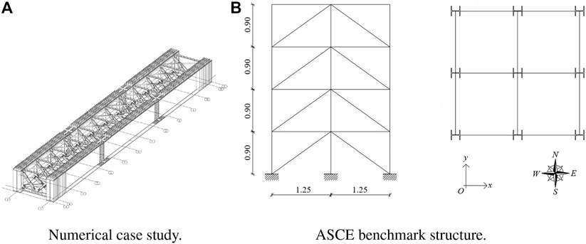
FIGURE 1. View of (A) the steel railway bridge representing the numerical case study and of (B) the ASCE benchmark steel braced frame. For the sake of clarity, the concrete slab is not shown in (A).

Once the dataset of modal features has been generated, another important aspect is to tune the hyper-parameters of the network such as to guarantee its best performance. In this regard, the choice of suitable approaches for the hyper-parameter search and for the dataset subdivision is motivated and described.

ANN have been proved to be capable of working with uncertain and noise-corrupted data (Khan and Yairi, 2018). However, when the level of noise is such to cover the effect of the system modification over the input features, a rapid decrease of performance is expected. For this reason, a white noise process with a significant noise level is added to the structural response of both models. At the same time, a multivariate statistics technique, namely the PCA, is applied for noise-filtering and a comparison between networks that use noise-corrupted data and filtered data is performed. In summary, to calibrate the network and to test the effectiveness of the neural network for damage detection, the fundamental steps of the proposed procedure are the following.

• Select the case study, obtain the reference dataset of modal properties in the undamaged condition (from the response of model R for the numerical case study and from the experimental measures for the real case study) and built the support model (model S);

• Generate the dataset for the network training from the numerical model (model S) and collect the dataset for the network test from the real structure (experimental data) or from the model R (in the case of pseudo-experimental data);

• Apply noise filtering of the data with principal component analysis to obtain a cleaned database;

• Perform the hyper-parameters tuning and the training of the final networks;

• Test the networks with new data (simulated or measured) to assess the effect of model and measurements errors.

All the procedure details are presented in the next section with reference to the numerical case study.

4 Numerical case study

In this section, the proposed procedure, described in Section 3, is applied to a numerical case study. The case study is a steel railway girder bridge approximately 40 m long and 4.3 m wide. Two simple supported steel girders carry a concrete slab 34 cm thick. The slab is connected to the top flanges of the girders through pegs that prevent the slip between the adjacent surfaces. The two steel girders are connected to each other by a complex bracing system. It is a three-dimensional system composed of a basic 3D truss, whose dimensions are 3.5 m × 2.4 m × 2.4 m, that recurs for the whole length of the bridge. A 3D view of the girders and of the bracing system is reported in Figure 1A.

4.1 Numerical modelling and calibration

A detailed FE model of the railway bridge is developed using the FE software MIDAS CIVIL. This model is adopted to create the dataset replacing the experimental observations in the undamaged state as well as to test of the networks in the last phase of the procedure. Flanges and webs of the steel girders and the concrete slab are modelled with shell elements, while beam and truss elements are used for the bracing system. The top flanges of the girders are connected to the concrete slab through rigid links. Thicknesses of the plate elements are chosen according to the dimensions of the modelled member. The value of the elastic modulus assumed for concrete and steel is 31475 MPa and 210000 MPa, respectively. The typical restrain condition of a bridge involves the use of hinges and rollers in order to allow the thermal deformations of the bridge in the two horizontal directions, while the displacement in the vertical direction are prevented. When the amplitude of the excitation is small, as in the case of environmental excitation, the displacement of the rollers are expected to be negligible due to the friction within the support system. For this reason, the restrain conditions are imposed at the extremal sections of both the girders by preventing the displacements of the nodes of the bottom flanges in all directions, while rotations are allowed.

A simpler model (model S) has been developed for the generation of the network training dataset. The model S is a simply supported beam with 100 finite elements characterized by an equivalent rectangular cross section. Each beam element has both flexural and shear deformability. The properties of the cross section are defined through the calibration procedure described below.

Natural frequencies and mode shapes of both FE models are obtained performing modal analysis and modifying the exact values of the structural response by adding noise with the aim to reproduce measurement errors and uncertainties characterizing the modal identification procedure. A dynamic monitoring system is assumed to be installed on the bridge. The measurement equipment is supposed to be composed of five accelerometers (A1-A5) connected to the structure and placed along the bridge length at specific locations. With respect to the numeration A1-A5, the locations are at 6, 13, 20, 27 and 34 m from the left extremity of the bridge. Therefore, the mode shape components are available only for the points corresponding to the sensor locations. A Gaussian noise with a coefficient of variation depending on the property type is added to the exact values computed by the models. It is assumed that the temperature effects on modal properties have been filtered out through, for instance, the procedure presented in Comanducci et al. (2016), Maes et al. (2022). Therefore, the introduced Gaussian noise represents the residual variability. The coefficient of variation is set to .01 for frequencies and .05 for mode shapes. Moreover, to introduce non-negligible uncertainties also for near-zero components of mode shapes, a further specific source of error is introduced by adding a noise extracted from a uniform distribution.

The values of the elastic and shear modulus of model S are calibrated with respect to the response of model R. In particular, these parameters are chosen with the aim to minimize the discrepancy function e_F, that reads:

where f_R,m denotes the mth frequency of the model R in its undamaged condition and f_S,m denotes the corresponding frequency of model S computed for the values of the updating parameters collected in the vector θ. M is the number of considered natural frequencies, in this case the frequencies of the first four vertical bending modes. The function e_F thus represents the discrepancy between the frequencies computed by the two models. Mode shapes have not been included in the calibration since they are not sensitive to the modification of the chosen structural parameters, which are uniform along the bridge length. The calibration procedure has been carried out with a surrogate-assisted evolutionary algorithm that employs an improved sampling strategy (Vincenzi and Gambarelli, 2017; Ponsi et al., 2021). The calibrated natural frequencies of model S are compared to the frequencies of model R in Table 1. As a consequence of the different modelling strategies adopted, a residual discrepancy persists also after the calibration. The same goes for the mode shapes as shown in Figure 2, where the comparison for mode two and three is presented.

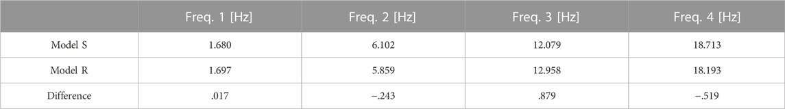
TABLE 1. Numerical case study: comparison between natural frequencies of model S and R after calibration.

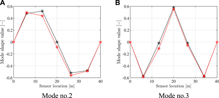
FIGURE 2. Numerical case study: comparison between mode shapes computed by model S (black asterisks) and model R (red asterisks); (A) mode no. 2 and (B) mode no. 3.

4.2 Damage scenarios

Damage is simulated in both models through the reduction of the elastic modulus of one or more finite elements. Considering the elastic modulus E_u of an undamaged element and the reduced elastic modulus E_d of a damaged element, it is possible to define the damage severity r as:

As concerns model S, several damage scenarios are created by varying damage severity and location of a single damaged element, that may assume different values. In detail, damage location varies with a step-size of 5% of the bridge length over the whole structure, while its severity varies from 0% to 40% with a step-size of 2.5%. The structure condition is considered as lightly damaged if the severity of damage is lower than 15%, otherwise it is considered as severely damaged. Considering the stochastic modelling of measurement errors, 200 samples compose the dataset for each damage scenario. The single sample is obtained by adding the randomly extracted values of noise to the exact value of the modal response. The response of the model for the undamaged scenario is repeated a number of times equal to 1/3 of the number of simulations in the damaged conditions. In this manner, the sizes of the datasets related to the three classes are comparable.

Finally, seven further scenarios are created for model R. The first represents the undamaged state of the model, while the remaining six are the damage scenarios described in Table 2. For each damage scenario, Table 2 defines the damaged element and the damage location and extension. Damage in the steel beam (with reference to scenarios S2, S3 and S4) is introduced by decreasing the elastic modulus of an element row of the bottom flange to a quasi-zero value, aiming at simulating material discontinuity. For scenarios involving damage of the concrete slab, i.e. S5, S6, and S7, the elastic modulus of concrete is reduced by 50% to simulate a cracked condition. In S5 and S6 a whole element row along the slab width is damaged, while in S7 a nearly semi-circular area of the concrete slab is damaged.

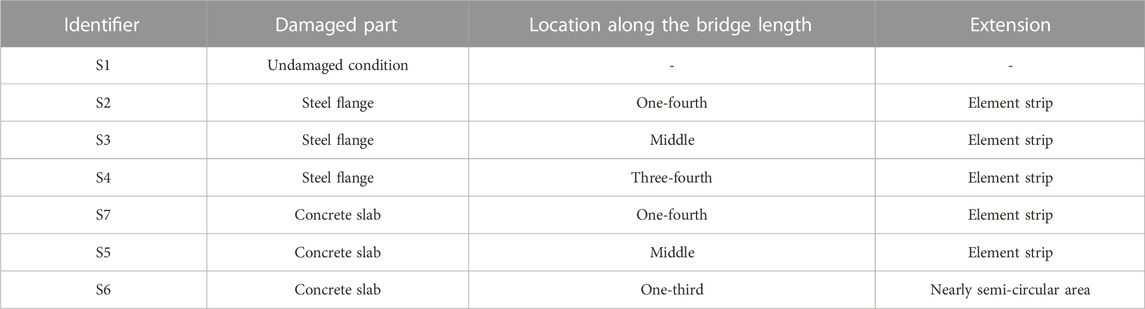
TABLE 2. Numerical case study: description of the damage scenarios of model R.

4.3 Network definition

This section describes the networks employed in the procedure, with reference to the construction of the input vector of the MLP. These networks, together with their identifiers and main features, are listed in Table 3. All these networks have an input vector composed of the natural frequencies of the four bending modes followed by the corresponding mode shape components. Only the mode shape components corresponding to the five sensors of the monitoring system (A1-A5 defined in Section 4.1) are considered, resulting in a input vector of dimensions 24 × 1. As explained in the same section, noise is added to the exact values of the modal features to account for measurements errors and uncertainties in the identification procedure. Thus, the network input becomes a 24 × N matrix, being N the number of modal parameter sets considered.

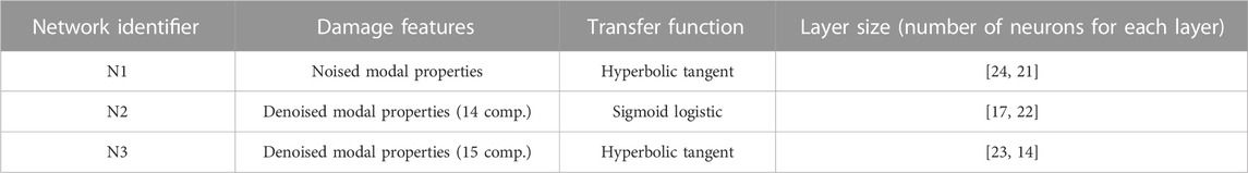
TABLE 3. Numerical case study: studied networks and their optimal architecture.

In this work, three different networks are investigated that stand out for the preprocessing of the dynamic features given as input. The network N1 takes as input noise-corrupted modal properties, while for network N2 and N3 a noise filtering is performed through the PCA (see Table 3).

The PCA is a well-known technique of multivariate statistics that is usually employed for data compression or noise filtering. First, a large set of variables is transformed into a smaller one that contains most of the information stored in the large set. The loss of information is accepted in order to visualize and analyse data in a simpler manner. Principal components are linear combinations of the original variables, realized in such a way that the new variables are uncorrelated and most of the information contained in the original variables is compressed into the first new variables. By reversing the transformation and retaining only the most important components, it is possible to filter the noise affecting the original variables. The fundamental steps of PCA are briefly described in the following.

• Normalization of data in order to avoid that variables characterized by larger standard deviations dominate the process. For a given variable x_i, that in this work is a component of the MLP input vector, with mean μ_i and standard deviation σ_i, the normalized variable z_i (i = 1, … 24) is obtained as:

Normalized data can be organized in columns forming the matrix Z.

• Identification of the correlations between variables through the computation of the covariance matrix $\mathbf{\Sigma }\left(\mathbf{Z}\right)$;

• Computation of the eigenvalues s_i and the eigenvectors l_i of the covariance matrix Σ. The eigenvectors represent the principal components, while the corresponding eigenvalues give the amount of variance in each principal component.

• Discarding the components of lower significance on the basis of the relative amount of variance rv_i:

In particular, the eigenvectors are ordered based on the descending value of the corresponding eigenvalue. The matrix that stores the eigenvectors as columns is denoted by L. There is no a fixed rule for discarding the components of lower significance, since the operation highly depends on the available data. A common practice is to keep the first p principal components that allow to retain almost the 95% of total amount of variance, namely

The selected components organized by columns will form the loading matrix L_P.

• Transformation of the data along the principal component axes

After the transformation, most of the information contained in the original data is described with a lower number of variables. Matrix T is denoted as score matrix and its elements as principal component scores.

• Reconstruction of the original variables through the loading matrix L_P, discarding the last principal components whose variability is associated to noise:

A baseline set of frequencies and mode shapes is created considering only data referred to the undamaged state. The matrices Z_f and Z_ϕ for frequencies and mode shapes have dimensions N_f × M_und and N_ϕ × M_und, respectively. N_f and N_ϕ are the number of frequencies and mode shape components considered, while M_und is the number of samples composing the undamaged dataset. Then, PCA is separately applied to the frequency and mode shape sets in order to compute the loading matrices L_P,f and L_P,ϕ. At the end, data are reconstructed in the original coordinate system using Eq. 11. The core of the problem lies in the choice of the number of principal components to retain. In this instance, frequency set is analysed: each principal component describes about 25% of the total variance. Consequently, all the four principal components are retained and the original data are conserved. As concerns mode shapes, the cumulative percentage of variance described by the principal components is represented in Figure 3. The cumulative percentage of variance described by retaining 14, 15 or 16 principal components is 91.5%, 96.0%, and 99.9%, respectively. Since the value of 99.9% is high and is likely that it includes the variability due to noise, only the cases of 14 or 15 principal components are selected. In the first case (14 components) the reconstructed data form the input vector of network N2, while 15 components are selected for the network N3. It is worth noticing that baseline sets are composed of only data related to the undamaged scenario, but the operation of noise filtering is applied also to the dataset of the damaged scenarios.

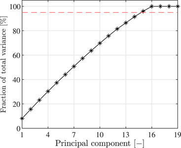
FIGURE 3. Numerical case study: cumulative percentage of total variance explained by the principal components of the mode shape baseline. Red dashed line: threshold value of 95%.

4.4 Architecture optimization

The architecture optimization involves the tuning of a series of hyper-parameters in order to improve as much as possible the performance of a network. The optimization is performed by means of Randomized Grid Search (Bergstra and Bengio, 2012) and k-fold Cross Validation (Arlot and Celisse, 2009). They are described referring to a generic network, but the procedure is applied to all the networks defined in Section 4.3. Randomized Grid Search is a strategy of hyper-parameter search that is very diffused in the Machine Learning community. First, it is necessary to select the hyper-parameters to be tuned and their range of variation. In this case the hyper-parameters considered are the number of hidden layers, their size and the type of transfer function used. The hidden layers can be one or two, their size may vary between the dimension of the output vector and the dimension of the input vector. In the present study, the dimension of the output vector is 3, corresponding to the three possible damage conditions, namely undamaged, lightly damaged and severely damaged, while the dimensions of the input vector is 24. As introduced in Section 2, the possible transfer functions are: the Sigmoid logistic function, the hyperbolic tangent function and the rectified linear unit (ReLU) function. The combinations of all the possible values that each hyper-parameter can assume, based on the range of variation previously defined, are realized by creating a grid. Trying out all the possible combinations of the grid can be very time-consuming so a randomized strategy is used instead. The Randomized Grid Search algorithm randomly extract a triplet of values for the hyper-parameters from the grid and evaluates the related network performance. This operation is repeated for a fixed number of times and the optimal hyper-parameter combination will be the one that provides the best network performance.

The network performance is evaluated by means of k-fold Cross Validation. This approach represents an evolution of the classic approach based on the simple split of the whole dataset in training, validation and test subset. These subsets remain unchanged once they have been defined. However, the network performances are highly dependent on the training and the validation set. The network may perform very differently when it is trained and evaluated on a different subset of data. The idea behind k-fold Cross Validation is to repeat training and validation on different subsets of the data. Initially, the whole dataset is split into a subset dedicated to the cross validation and an hold-out subset. The latter is not involved in cross validation and it will be employed after the tuning to assess the network generalization. With reference to the dataset described in Section 4.2, the 2% of the undamaged dataset and of the damaged dataset are used to construct the hold-out set, while the remaining data of the undamaged and damage scenarios compose the cross validation subset. This subset is further split into k folds. The evaluation of the network performance consists of k iterations: at each iteration the kth fold is used as validation set and all the remaining folds are used as training set. The process is repeated until every fold has been used as validation set. At each iteration, a performance score is obtained. It is the value of the network loss function (Eq. 4) computed on the validation set. The overall performance score is given by the average value of all the k scores. By training and testing a network with the k-fold cross validation, we get a more accurate representation of how well the network might perform on new data. Once the optimal hyper-parameters values are found, they are employed to construct the final network that is subsequently trained on the whole cross validation set. Finally, the trained model is tested on the hold-out set.

Results of the architecture optimization for the numerical case study are shown in the following. The optimization has been performed in accordance with the Randomized Grid Search and k-fold Cross Validation approach, both of them described in Section 4.4. The Randomized Grid Search has been implemented by extracting 100 random triplets of hyper-parameter values from the grid, namely the number of layers, their size and the transfer function, for each network type. First, some qualitative observations about the influence of the hyper-parameters on the network performance are drawn. Focusing on the samples characterized by a single layer, Figure 4 shows the loss function of the networks N1 (Figure 4A) and N2 (Figure 4B) based on the number of neurons in the layer. In both cases, regardless of the transfer function type, the loss function value decreases with the number of neurons increment. For a fixed number of neurons, the performance obtained with a Sigmoid logistic function and hyperbolic tangent function are better than those obtained with a ReLU function. In the case of network N2 (Figure 4B) the difference is more marked compared to network N1 (Figure 4A). No result is shown for network N3 since the behaviour is very similar to that of N1.

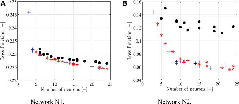
FIGURE 4. Numerical case study: performance of the networks with a single hidden layer in function of the number of neurons and the transfer function type; (A) Network N1 and (B) Network N2. Black •: ReLU transfer function; blue +: Sigmoid logistic transfer function; red ∗: hyperbolic tangent transfer function.

Figure 5 shows the loss function values for the cases where the networks are characterized by two hidden layers. In general, the use of a second hidden layer improves the performance of all the networks: it can be easily noted comparing the minimum values of Figure 4 and Figure 5. For network N3 (Figure 5B) the performance score obtained with the ReLU function is always larger than the scores obtained with sigmoid logistic and hyperbolic tangent function. The same considerations are valid for N2 (Figure 5B) even if the differences in terms of performance scores are reduced. The optimal architectures found are indicated in Table 3. According to the previous observations, for all the networks they are composed by two hidden layers and they are not characterized by the ReLU transfer function.

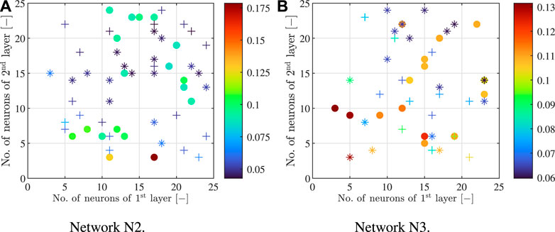
FIGURE 5. Numerical case study: performance of the networks with two hidden layers in function of the number of neurons in each layer and the transfer function type; (A) Network N2 and (B) Network N3. •: ReLU transfer function; +: Sigmoid logistic transfer function; ∗: hyperbolic tangent transfer function.

4.5 Training and test of the final networks with the dataset of model S

Once the optimal architecture has been found, the final networks N1, N2, and N3 are trained over the whole cross validation set and tested over the hold-out set, that has not been part of the dataset used for hyper-parameter tuning. The trained networks are compared in terms of accuracy and percentage of uncertain predictions. The accuracy is a measure of the errors that a network commits and it derives from the comparison between network predictions and the associated target class. The accuracy of each network is calculated with reference to two different criteria, namely a “strict” and a “soft” accuracy.

The strict accuracy is obtained when the predicted output exactly corresponds to the target. The analysis of the strict accuracy of the final networks N1, N2, and N3 can be performed thanks to the confusion matrices that are shown in Figure 6. For each network, the confusion matrix is computed with reference to the training dataset (Figures 6A,C,E) and to the test dataset (Figures 6B,D,F). The overall strict accuracy value of each matrix can be seen in the matrix corner located in the right-bottom angle. The same values are summed up in Table 4. Analysing a generic matrix along columns, it is possible to see how the subset of data that has a specific target class, identified by the column, has been classified by the network. Conversely, along a row it is possible to see which are the target classes of the data that have been classified in that way by the network. Combining the information along the columns and rows, it follows that the main diagonal of the matrix contains the samples correctly recognized in each class.

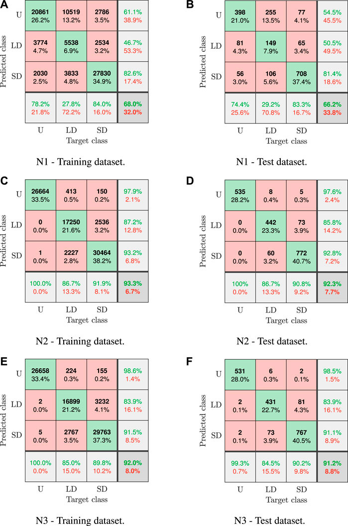
FIGURE 6. Numerical case study: confusion matricies of the trained final networks N1, N2, and N3 computed for (A,C,E) the training dataset and (B,D,F) the test dataset. U, undamaged; LD, light damage; SD, severe damage.

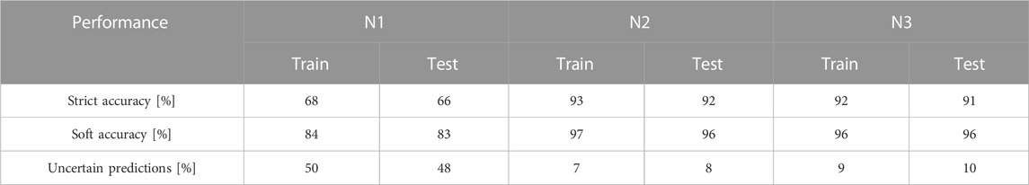
TABLE 4. Numerical case study: performances of networks N1, N2 and N3 for the dataset of model S.

As a general observation valid for all the networks, the difference between the matrices computed for the training and the test dataset is very limited. This confirm the high level of generalization reached by the networks and it excludes over-fitting of data. Matrices of networks N2 and N3 are similar (Figures 6C–F), so the same considerations can be formulated: a practically zero percentage of samples whose target class is the undamaged condition is mistakenly classified in a damaged condition, while the principal error source is due to the classification of samples whose target class is the low damage condition in the severe damage condition, or vice versa. The analysis for N1 is different, since the predominant error committed is the classification as undamaged of samples with low damage target condition. This is the main reason of the bad accuracy of N1.

According to the criterion of the soft accuracy, a tolerance of 5% to the damage severity boundaries reported in Section 4.2 for the three classes is applied. If the classification output is not correct but the damage severity is included in the tolerance range, the mistake made is considered light. Therefore, the “soft accuracy” takes into account only errors that are out of the tolerance range. The values of the “soft accuracy” are summed up in Table 4. For all the networks, this value is larger than the “strict accuracy” value, confirming how a fraction of mistakes committed by the networks are light in the sense that has been previously explained. The increment obtained moving from “strict accuracy” to “soft accuracy” is more marked for network N1.

The percentage of uncertain predictions is computed considering the probability expressed by the output layer of the MLP. Let y_ord = [p₁, p₂, p₃] be the output vector of the network with probabilities ordered in descending order (i.e. p₁ > p₂ > p₃) associated to each class. If a small gap is found between the probability p₁ and p₂, the damage class is defined with higher uncertainty with respect to the case when p₁ ≫ p₂. For this reason, a threshold value μ equal to .33 is defined, which discriminates certain predictions from uncertain ones. When p1 − p2 < μ the result is considered uncertain. The percentage of uncertain predictions listed in Table 4 agree with the considerations formulated focusing on the accuracy values: the performance of network N1 is the worst, since it has a percentage of almost 50% of uncertain predictions. On the contrary, N2 and N3 are characterized by values equal or smaller than 10%.

In conclusion, the noise-corrupted modal properties taken as input by N1 do not allow to clearly identify damage because the effect of noise covers the variation of modal properties caused by damage. When PCA is applied to filter noise, as in the case of N2 and N3, very good values for accuracy and percentage of uncertain predictions are obtained. The choice between 14 or 15 principal components for the construction of the loading matrix does not produce substantial differences in this phase.

4.6 Test with the dataset of model R

Test with model R is realized with the aim to investigate the effect of the model error on the accuracy of networks N1, N2, and N3. First, the exact values of modal properties computed by model R, thus without introducing measurement errors, are provided to the networks. The first part of Table 5 collects the classification results of the seven scenarios listed in Table 2. All networks identify all scenarios as damaged, including the scenario S1 that corresponds to the undamaged state of the detailed model R. The model error is evidently the cause of these bad results. Although model S has been calibrated based on the response of model R, residual errors still remain both for natural frequencies (Table 1) and mode shapes, as highlighted in Figure 2 for mode 2 and 3. These residual errors are interpreted by the networks as variations of the modal properties with respect to the target undamaged condition.

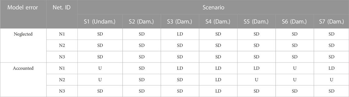
TABLE 5. Numerical case study: results of the test with model R considering or not the model error. U: undamaged condition; SD: severe damage; LD: light damage.

A proposal is here presented in order to prevent the misclassification of the undamaged condition due to the model error. The residual error obtained at the end of the calibration must be added to the modal properties computed by the reference model (model R or, in real case studies, the experimental modal properties). The residual error has to be applied for all the structural conditions, both undamaged and damaged, despite it was computed referring only to the undamaged state. There is no guarantee that the residual error does not change when the structure is damaged, but its computation for different damage scenarios is not feasible in almost all real applications. Moreover, the proposal to adjust the network input data by adding the residual term aims to cut down the effect of model error for the undamaged condition. In the authors’ opinion, it is of less relevance if it slightly alters the prediction of modal properties in the damaged condition.

The classification results obtained accounting for the model error are presented in the second part of Table 5. As concerns N1 and N2, the first four scenarios are correctly identified. Scenarios involving damage in the concrete slab (S5, S6, and S7) are correctly identified by the network N1 except for S6, while the network N2 identifies all of them as undamaged. This result confirms that identifying local damage of the concrete slab is not an easy task. There is no improvement in the predictions of network N3, since they are basically the same of the first part of Table 5. The false alarm related to the misclassification of scenario S1 is not avoided.

The behaviour of the networks with reference to the identification of the undamaged condition is analysed also by adding the measurement noise. In particular, the exact values of modal properties computed by model R are corrupted by a Gaussian noise. The frequency and the mode shape coefficients of variation (CVs) varies in the range [1%, 10%]. For each value of the CVs, 100 samples of pseudo-experimental data are extracted and the predictions of networks N1 and N2 are computed. Network N3 is not considered in this analysis since it is not able to correctly identity the undamaged condition also when exact modal properties are employed. The plots of the network accuracy in function of the frequency and mode shape CVs are illustrated in Figure 7. Both the plots are not smooth but a clear trend can be detected. An increase in the frequency and mode shape CVs, namely an increase of the noise amplitude, determines a reduction of the accuracy of N1 and N2. However, the entity of this reduction is very different. The accuracy of N1 is insufficient for a large part of the domain of Figure 7A and the minimum value is around 10%. On the other hand, the accuracy of N2 is larger than 70% for almost the entire plot, with the only exception of the part of the domain characterized by the highest values of both frequency and mode shape CVs (see Figure 7B). Finally, the accuracy of both N1 and N2 has proved to be more sensitive to the increment of mode shape CV, even if it is not completely insensitive to the frequency CV. This behaviour could be caused by the fact that the input vector of the networks is composed in largest part by the mode shape components (20) compared to the natural frequencies (4).

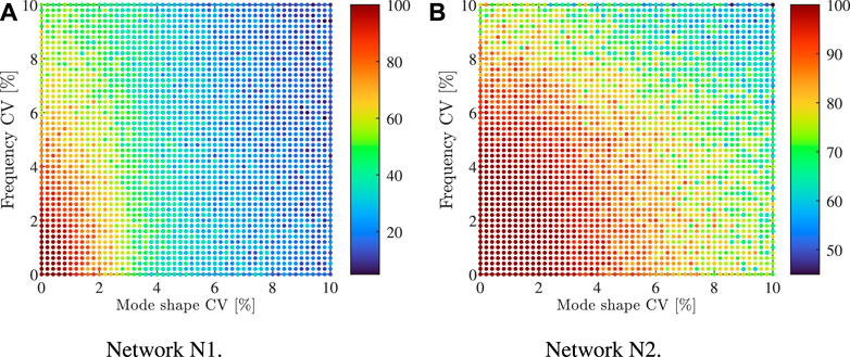
FIGURE 7. Numerical case study: plot of the accuracy of the network (A) N1 and (B) N2 for different values of the frequency and mode shape coefficient of variation (CV).

5 ASCE benchmark structure

In this section, the damage detection procedure described in Section 3 is applied to a real case study, namely the steel braced frame employed as benchmark problem for SHM purposes by the IASC-ASCE SHM Task Group in the early 2000s (Dyke et al., 2001; 2003).

5.1 Description of the structure and the experimental test

The structure has four stories with an overall height of 3.6 m and a 2-bay by 2-bay plan of dimension 2.5 m × 2.5 m. The structural elements are composed of columns, floor beams and braces, while each floor is composed of four slabs, one for each bay. A schematic plan view where the orientation of the column section is delineated with respect to a x-y coordinate system can be found in Figure 1B. Further details about the properties of the structural element sections, that are unusual because they have been designed for a scale model, and the values of the floor masses can be found in Johnson E. et al. (2004).

This structure was located at the Earthquake Engineering Research Laboratory at the University of British Columbia and was subjected to several experimental tests. The different tests are characterized by different structural configurations. The first one is the fully braced configuration described in the previous paragraph, while the remaining configurations can be considered as damaged scenarios of the first structural condition since specific braces are removed. Five damage configurations are the object of this study. They are denoted with the numbers 2–6. In configuration two the braces located at all floors in the East side are removed. For the configurations three to five the focus is addressed to the braces located in the South-East corner. Braces of all floors are removed for configuration 3, braces of the first and fourth floor are removed for configuration 4, while only those of the first floor are removed for configuration 5. Finally, configuration 6 is characterized by the removal of the braces of the second floor on the North side.

For each configuration, the structure has been tested exploiting an environmental source of excitation. For each frame floor, including its base, three accelerometric sensors were employed and disposed in almost the same positions. With reference to the plan view represented in Figure 1B, sensors are located in proximity of the central alignment of columns that is parallel to the y-axis. The central sensor measures accelerations along the y direction, while the other two measure accelerations along the x direction. More details about the specifics of the instrumentation and the tests can be found in Dyke et al. (2003).

The dynamic identification of the frame modal properties for all the configurations has been performed by the authors of this work. The modal extraction has been carried out with the Stochastic Subspace Identification (SSI) method (Overschee and Moor, 1996; Peeters and De Roeck, 1999). The identified modes and their natural frequency are listed in Table 6 for all the configurations.

TABLE 6. ASCE benchmark structure: natural frequencies in Hz of the identified modes for the different configurations. B1: first bending mode; B2: second bending mode; T: torsional mode; x or y: mode direction.

5.2 Numerical modelling and calibration

The FE model of the frame adopted for ANN dataset generation is obtained thanks to the MATLAB based FE code released by the IASC-ASCE SHM Task Group and available at the web site http://datacenterhub.org/. The columns and the beams are modelled as Euler-Bernoulli elements and the braces as truss elements. The connections among columns and beams are able to transfer the bending moment. The in-plane rigid floor behaviour has been considered by constraining the horizontal translations and the rotation in the floor plane of the nodes in each floor to be the same. In total, the model has 120 degrees of freedom. The FE code allows computing compute mass and stiffness matrices and provides the implementation of a lumped mass matrix.

If the nominal values of material and geometrical properties of the elements are used for the model, as provided in the Matlab code, there is a remarkable difference between the experimental and numerical frequencies. For this reason, a calibration procedure has been implemented in order to reduce as much as possible the differences. The elastic modulus of the elements, whose value is the same for columns, beams and braces, is tuned with this aim. In this way, only the natural frequencies can be adjusted, while mode shapes are insensitive to a uniform modification of a stiffness property in the whole structure. Other strategies could be adopted in order to increase the correlation between experimental and numerical mode shapes [see for instance Ponsi et al. (2021; 2022)]. In this work, the authors aim at showing that the proposed procedure is effective also in the case of residual differences between the modal parameters after the calibration procedure. For this reason, a more complex calibration strategy is not adopted. The comparison between the calibrated modal properties and their experimental counterparts is shown in Table 7. It can be seen how there is an almost exact correspondence for the frequencies of the first two modes, while larger errors are obtained for the last three modes, with a maximum of 11% for the torsional mode. As regard mode shapes, a good correlation is found for all the modes.

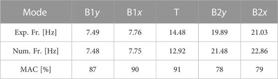
TABLE 7. ASCE benchmark structure: comparison between the experimental and the calibrated numerical modal properties of the steel braced frame. B1: first bending mode; B2: second bending mode; T: torsional mode; x or y: mode direction.

5.3 Dataset generation

The calibrated FE model of the frame is used for the generation of the dataset dedicated to the network training and test. The dataset is composed of the modal properties computed by the model in its undamaged condition, namely the condition characterized by the values of the model parameters that have been found thanks to the calibration, and by the modal properties related to different damage scenarios. The scenarios have been created by simulating damage on each brace of the frame. Only the braces are considered as possible damaged elements since the experimental damaged configurations are limited to these elements. Damage is simulated by reducing the elastic modulus of a brace of a specific quantity expressed by the damage severity (see Eq. 6). The latter ranges in the interval [0%, 90%] with step size 10%. For each damage scenario, 200 samples are generated by adding measurement noise (Gaussian noise) to the exact values of modal properties. The coefficients of variation for frequencies and mode shapes are set to 1% and 5%, respectively. The same operation is performed for the undamaged condition of the model, but in this case the number of sample is greater, in such a way that the size of the undamaged scenario is about 1/3 of the size of the whole dataset.

5.4 Network definition, training, and test

As a fist trial, only a single network is studied for the ASCE benchmark. This network has an input vector composed of the natural frequencies of the five modes described in Section 5.1, followed by the corresponding mode shape components. Only the mode shape components corresponding to the sensors of the monitoring system are considered, resulting in a input vector of dimensions 80 × 1. No filtering technique has been applied to the data before network training and a single network architecture has been considered. The network has two hidden layers, each of them composed of 30 neurons and characterized by a hyperbolic tangent function. The results of the k-fold cross-validation, that has been performed in compliance with the description of Section 4.4, are very satisfactory. Indeed, for each of the five iterations where one of the five fold is alternately selected as validation set, the accuracy is larger than 98%. Due to the excellent results, PCA (Section 4.3) is not applied to filter noise and the architecture optimization (Section 4.4) is not performed. Nevertheless, if the accuracy values were unsatisfactory, the previous techniques could be applied without further complications compared to the numerical case study of Section 4.

As a last step, the final network has been trained on the whole set used for cross-validation and tested on the hold-out set. The accuracy of the training set is very high, namely 99.8%, and also for the test set an excellent value is obtained (98.7%). A very small percentage of samples whose target class is the severe damage condition are misclassified in the light damage condition, and vice versa. On the other hand, the target undamaged samples are almost always classified in a correct way. The results of the test with the experimental data described in Section 5.1 are presented in Table 8. The behaviour is the same observed in Section 4.6, i.e. when model error is neglected the network classifies all the configuration, including the undamaged one, in the severe damage condition. Conversely, the addition of model error to the experimental data enables to correctly classify the undamaged configuration (1) and the damaged configurations (2–6) as severe damage conditions.

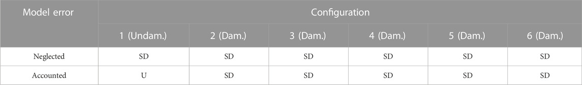
TABLE 8. ASCE benchmark structure: results of the test with the experimental data. U: undamaged; LD: light damage; SD: severe damage.

6 Conclusion

This paper presented a neural network-based damage identification procedure that employs modal properties as damage sensitive features. Particular emphasis is given to the importance of accounting for the model error in the damage detection procedure. In civil engineering applications, indeed, it is not feasible to obtain large amount of data relative to damaged conditions to train the network. As a consequence, finite element models need to be employed to simulate damaged scenarios. The unavoidable differences between the real structure and the numerical model, although small, compromise the efficiency of the damage detection procedure. Two case studies are analysed with the aim of showing both the effectiveness and the suitability to different applications of the proposed procedure. The first case study is a steel railway bridge and in this case only simulated data are considered. The second case study is the ASCE benchmark steel braced frame. Although the analyses related to the first case study are based on simulated data only, a series of key aspects are taken into account to ensure that results are representative of real applications. In particular, a Gaussian noise is added to simulate measurement errors and identification uncertainties and two numerical models are developed to account for model error. Model R is a detailed finite element model of the bridge that is adopted to represent the real structure and generate the pseudo-experimental observations, while model S, simpler than model R, is calibrated with respect to model R and employed to create datasets relative to different damage scenarios to train the networks.

Dealing with the numerical case study, damage detection has been performed adopting three different networks, one assuming as input noise-corrupted modal properties (network N1) and the others using noise-filtered modal properties (networks N2 and N3). Noise filtering has been carried out by means of the Principal Component Analysis technique. As concerns the training and test phase with model S, network N1 has shown the worst performances, while N2 and N3 have presented large values of accuracy and low percentages of uncertain predictions. The test phase with model R has highlighted the need to account for the model error. Being the networks calibrated with reference to data generated from model S, they are not able to identify the undamaged condition when dealing with data from model R, as they recognize the difference between the modal properties of the two models as damage. On the contrary, if the input data are corrected with the residual error obtained after the model calibration, networks N1 and N2 correctly identify the healthy state and the presence of damage on the steel beam. Damage on the concrete slab has been more difficultly identified. Finally, results obtained by also adding measurement noise have shown for N2 a limited reduction of the accuracy with an increasing level of noise. Results obtained for the ASCE benchmark structure are consistent with those obtained from the numerical case study. In this case, a single network was defined, that assumed non-filtered modal properties as input. The great level of damage introduced in the experimental tests and for the creation of the network dataset, namely the damaging or the complete removal of a single or a group of braces, made the noise effect on the modal properties negligible compared to the effect of damage.

To sum up, presented analyses highlighted the importance of accounting for the model error in the damage identification procedure. If neglected, the model error is identified as damage due to the unavoidable differences between the real structure and the finite element model required to train the network. The procedure proposed in this paper is well suited to real-time damage identification. This is made possible by the use of black box modelling such as neural networks, as in this case the time-consuming part of the procedure (namely the network training) is performed in a preliminary phase before the actual monitoring. This would not be possible with damage identification methods based on physical modelling, being them very time consuming in real applications. Moreover, the use of noise-free data is often essential to avoid false identification of damaged scenarios, especially when the amplitude of noise is comparable to that of the changes induced by damage. In this context, Principal Component Analysis is one of the simplest, efficient and fast numerical method to achieve these goals and define a truly real-time procedure.

Data availability statement

The raw data supporting the conclusions of this article will be made available by the authors, without undue reservation.

Author contributions

FP and EB contributed to conception and design of the study. FP organized the database and performed the simulations. All authors contributed to the interpretation of results. LV supervised the work. EB and FP wrote the first draft of the manuscript. All authors contributed to manuscript revision, read, and approved the submitted version.

Conflict of interest

The authors declare that the research was conducted in the absence of any commercial or financial relationships that could be construed as a potential conflict of interest.

Publisher’s note

All claims expressed in this article are solely those of the authors and do not necessarily represent those of their affiliated organizations, or those of the publisher, the editors and the reviewers. Any product that may be evaluated in this article, or claim that may be made by its manufacturer, is not guaranteed or endorsed by the publisher.

References

Alves, V. N., de Oliveira, M. M., Ribeiro, D., Calçada, R., and Cury, A. (2020). Model-based damage identification of railway bridges using genetic algorithms. Eng. Fail. Anal. 118, 104845. doi:10.1016/j.engfailanal.2020.104845
Arlot, S., and Celisse, A. (2009). A survey of cross validation procedures for model selection. Stat. Surv. 4. doi:10.1214/09-SS054
Avci, O., Abdeljaber, O., Kiranyaz, S., Hussein, M., Gabbouj, M., and Inman, D. J. (2021). A review of vibration-based damage detection in civil structures: From traditional methods to machine learning and deep learning applications. Mech. Syst. Signal Process. 147, 107077. doi:10.1016/j.ymssp.2020.107077
Bakhary, N., Hao, H., and Deeks, A. J. (2010). Substructuring technique for damage detection using statistical multi-stage artificial neural network. Adv. Struct. Eng. 13, 619–639. doi:10.1260/1369-4332.13.4.619
Bartoli, G., Betti, M., Marra, A. M., and Monchetti, S. (2019). A bayesian model updating framework for robust seismic fragility analysis of non-isolated historic masonry towers. Philosophical Trans. R. Soc. A Math. Phys. Eng. Sci. 377, 20190024. doi:10.1098/rsta.2019.0024
Bassoli, E., Gambarelli, P., and Vincenzi, L. (2018a). Human-induced vibrations of a curved cable-stayed footbridge. J. Constr. Steel Res. 146, 84–96. doi:10.1016/j.jcsr.2018.02.001
Bassoli, E., Vincenzi, L., Bovo, M., and Mazzotti, C. (2015). “Dynamic identification of an ancient masonry bell tower using a MEMS-based acquisition system,” in Proceedings of the 2015 IEEE Workshop on Environmental, Energy and Structural Monitoring Systems, Trento, Italy.
Bassoli, E., Vincenzi, L., D’Altri, A. M., de Miranda, S., Forghieri, M., and Castellazzi, G. (2018b). Ambient vibration-based finite element model updating of an earthquake-damaged masonry tower. Struct. Control Health Monit. 25, e2150. doi:10.1002/stc.2150
Bergstra, J., and Bengio, Y. (2012). Random search for hyper-parameter optimization. J. Mach. Learn. Res. 13.
Betti, M., Facchini, L., and Biagini, P. (2015). Damage detection on a three-storey steel frame using artificial neural networks and genetic algorithms. Meccanica 50, 875–886. doi:10.1007/s11012-014-0085-9
Bianconi, F., Salachoris, G. P., Clementi, F., and Lenci, S. (2020). A genetic algorithm procedure for the automatic updating of fem based on ambient vibration tests. Sensors 20, 3315. doi:10.3390/s20113315
Brincker, R., Zhang, L., and Andersen, P. (2001). Modal identification of output-only systems using frequency domain decomposition. Smart Mater. Struct. 10, 441–445. doi:10.1088/0964-1726/10/3/303
Castagnetti, C., Bassoli, E., Vincenzi, L., and Mancini, F. (2019). Dynamic assessment of masonry towers based on terrestrial radar interferometer and accelerometers. Sensors 19, 1319. doi:10.3390/s19061319
Comanducci, G., Magalhães, F., Ubertini, F., and Cunha, Á. (2016). On vibration-based damage detection by multivariate statistical techniques: Application to a long-span arch bridge. Struct. Health Monit. 15, 505–524. doi:10.1177/1475921716650630
Doebling, S. W., Farrar, C. R., Prime, M. B., and Schevitz, D. W. (1996), Damage identification and health monitoring of structural and mechanical systems from changes in their vibration characteristics: A literature review. Los Alamos, NM: Communications Arts and Services Group (CIC-1) of Los Alamos National Laboratory. Technical Report LA-13070-MS.
Dyke, S., Bernal, D., Beck, J., and Ventura, C. (2003). “Experimental phase II of the structural health monitoring benchmark problem,” in Proceedings of the 16th ASCE Engineering Mechanics Conference.
Dyke, S., Bernal, J., Beck, C., and Ventura, C. (2001). “An experimental benchmark problem in structural health monitoring,” in Proceedings of the 3rd International Workshop on Structural Health Monitoring.
Figueiredo, E., Park, G., Farrar, C. R., Worden, K., and Figueiras, J. (2010). Machine learning algorithms for damage detection under operational and environmental variability. Struct. Health Monit. 10, 559–572. doi:10.1177/1475921710388971
Friswell, M. I. (2008). Damage identification using inverse methods. Vienna: Springer Vienna, 13–66.
Haykin, S. (1999). Neural networks: A comprehensive foundation. Englewood Cliffs, NJ: Prentice-Hall. International edition.
Hosamo, H., Nielsen, H., Alnmr, A., Svennevig, P., and Svidt, K. (2022). A review of the digital twin technologyfor fault detection in buildings. Front. Built Environ. 8, 1013196. doi:10.3389/fbuil.2022.1013196
Hou, R., and Xia, Y. (2021). Review on the new development of vibration-based damage identification for civil engineering structures: 2010–2019. J. Sound Vib. 491, 115741. doi:10.1016/j.jsv.2020.115741
Johnson, E., A., Lam, H., F., Katafygiotis, L., S., and Beck, J., L. (2004). Phase i iasc-asce structural health monitoring benchmark problem using simulated data. J. Eng. Mech. 130, 3–15. doi:10.1061/(asce)0733-9399(2004)130:1(3)
Khan, S., and Yairi, T. (2018). A review on the application of deep learning in system health management. Mech. Syst. Signal Process. 107, 241–265. doi:10.1016/j.ymssp.2017.11.024
Klepac, S., Subgranon, A., and Olabarrieta, M. (2022). A case study and parametric analysis of predicting hurricane-induced building damage using data-driven machine learning approach. Front. Built Environ. 8, 1015804. doi:10.3389/fbuil.2022.1015804
Lam, H. F., and Ng, C. T. (2008). The selection of pattern features for structural damage detection using an extended Bayesian ANN algorithm. Eng. Struct. 30, 2762–2770. doi:10.1016/j.engstruct.2008.03.012
Limongelli, M. (2010). Frequency response function interpolation for damage detection under changing environment. Mech. Syst. Signal Process. 24, 2898–2913. doi:10.1016/j.ymssp.2010.03.004
Luleci, F., Catbas, F., and Avci, O. (2022). A literature review: Generative adversarial networks for civil structural health monitoring. Front. Built Environ. 8, 1027379. doi:10.3389/fbuil.2022.1027379
Maes, K., Van Meerbeeck, L., Reynders, E., and Lombaert, G. (2022), Validation of vibration-based structural health monitoring on retrofitted railway bridge kw51. Mech. Syst. Signal Process., 165. doi:10.1016/j.ymssp.2021.108380
Møller, M. (1993). A scaled conjugate gradient algorithm for fast supervised learning. Neural Netw. 6, 525–533. doi:10.1016/S0893-6080(05)80056-5
Monchetti, S., Viscardi, C., Betti, M., and Bartoli, G. (2022). Bayesian-based model updating using natural frequency data for historic masonry towers. Probabilistic Eng. Mech. 70, 103337. doi:10.1016/j.probengmech.2022.103337
Mthembu, L., Marwala, T., Friswell, M. I., and Adhikari, S. (2011). Model selection in finite element model updating using the bayesian evidence statistic. Mech. Syst. Signal Process. 25, 2399–2412. doi:10.1016/j.ymssp.2011.04.001
Murtagh, F. (1991). Multilayer perceptrons for classification and regression. Neurocomputing 2, 183–197. doi:10.1016/0925-2312(91)90023-5
Osama, A., and Onur, A. (2016). Nonparametric structural damage detection algorithm for ambient vibration response: Utilizing artificial neural networks and self-organizing maps. J. Archit. Eng. 22, 04016004. doi:10.1061/(ASCE)AE.1943-5568.0000205
Overschee, P., and Moor, B. (1996). Subspace identification for linear systems. Theory - implemntation - applications. 1 edn. Springer.
Pandey, A., and Biswas, M. (1994). Damage detection in structures using changes in flexibility. J. Sound Vib. 169, 3–17. doi:10.1006/jsvi.1994.1002
Pandey, A., Biswas, M., and Samman, M. (1991). Damage detection from changes in curvature mode shapes. J. Sound Vib. 145, 321–332. doi:10.1016/0022-460X(91)90595-B
Pawar, P. M., Venkatesulu Reddy, K., and Ganguli, R. (2006). Damage detection in beams using spatial Fourier analysis and neural networks. J. Intelligent Material Syst. Struct. 18, 347–359. doi:10.1177/1045389X06066292
Peeters, B., and De Roeck, G. (1999). Reference-based stochastic subspace identification for output-only modal analysis. Mech. Syst. Signal Process. 13, 855–878. doi:10.1006/mssp.1999.1249
Ponsi, F., Bassoli, E., and Vincenzi, L. (2021). A multi-objective optimization approach for fe model updating based on a selection criterion of the preferred pareto-optimal solution. Structures 33, 916–934. doi:10.1016/j.istruc.2021.04.084
Ponsi, F., Bassoli, E., and Vincenzi, L. (2022). Bayesian and deterministic surrogate-assisted approaches for model updating of historical masonry towers. J. Civ. Struct. Health Monit. 12, 1469–1492. doi:10.1007/s13349-022-00594-0
Rainieri, C., and Fabbrocino, G. (2010). Automated output-only dynamic identification of civil engineering structures. Mech. Syst. Signal Process. 24, 678–695. doi:10.1016/j.ymssp.2009.10.003
Ramchoun, H., Ghanou, Y., Ettaouil, M., and Janati Idrissi, M. A. (2016). Multilayer perceptron: Architecture optimization and training.
Reynders, E. (2012). System identification methods for (operational) modal analysis: Review and comparison. Archives Comput. Methods Eng. 19, 51–124. doi:10.1007/s11831-012-9069-x
Ribeiro, A., Silva, J., and Maia, N. (2000). On the generalization of the transmissibility concept. Mech. Syst. Signal Process. 14, 29–35. doi:10.1006/mssp.1999.1268
Rosati, I., Fabbrocino, G., and Rainieri, C. (2022). A discussion about the douglas-reid model updating method and its prospective application to continuous vibration-based shm of a historical building. Eng. Struct. 273, 115058. doi:10.1016/j.engstruct.2022.115058
Rosenblatt, F. (1963). Principles of neurodynamics. perceptrons and the theory of brain mechanisms. Am. J. Psychol. 76, 705. doi:10.2307/1419730
Savoia, M., Vincenzi, L., Bassoli, E., Gambarelli, P., Betti, R., and Testa, R. (2014). “Identification of the manhattan bridge dynamic properties for fatigue assessment,” in Safety, Reliability, Risk and Life-Cycle Performance of Structures and Infrastructures - Proceedings of the 11th International Conference on Structural Safety and Reliability, ICOSSAR 2013, 12 January 2017, 4667–4674. Cited By :3 Export Date.
Sohn, H., Farrar, C. R., Hemez, F. M., and Czarnecki, J. J. (2002). “A review of structural health monitoring literature 1996–2001,” in Proceedings of the 3rd World Conference on Structural Control, Como, Italy.
Standoli, G., Salachoris, G. P., Masciotta, M. G., and Clementi, F. (2021). Modal-based fe model updating via genetic algorithms: Exploiting artificial intelligence to build realistic numerical models of historical structures. Constr. Build. Mater. 303, 124393. doi:10.1016/j.conbuildmat.2021.124393
Vincenzi, L., Bassoli, E., Ponsi, F., Castagnetti, C., and Mancini, F. (2019). Dynamic monitoring and evaluation of bell ringing effects for the structural assessment of a masonry bell tower. J. Civ. Struct. Health Monit. 9, 439–458. doi:10.1007/s13349-019-00344-9
Vincenzi, L., and Gambarelli, P. (2017). A proper infill sampling strategy for improving the speed performance of a Surrogate-Assisted Evolutionary Algorithm. Comput. Struct. 178, 58–70. doi:10.1016/j.compstruc.2016.10.004
Ying, X. (2019). An overview of overfitting and its solutions. J. Phys. Conf. Ser. 1168, 022022. doi:10.1088/1742-6596/1168/2/022022
Keywords: damage detection, data-driven methods, artificial neural networks, principal component analysis, model error
Citation: Ponsi F, Bassoli E and Vincenzi L (2023) Mitigation of model error effects in neural network-based structural damage detection. Front. Built Environ. 8:1109995. doi: 10.3389/fbuil.2022.1109995
Received: 28 November 2022; Accepted: 30 December 2022;
Published: 16 January 2023.
Edited by:
Giovanni Castellazzi, University of Bologna, ItalyReviewed by:
Cristina Gentilini, University of Bologna, ItalyFrancesco Clementi, Marche Polytechnic University, Italy
Copyright © 2023 Ponsi, Bassoli and Vincenzi. This is an open-access article distributed under the terms of the Creative Commons Attribution License (CC BY). The use, distribution or reproduction in other forums is permitted, provided the original author(s) and the copyright owner(s) are credited and that the original publication in this journal is cited, in accordance with accepted academic practice. No use, distribution or reproduction is permitted which does not comply with these terms.
*Correspondence: Elisa Bassoli, elisa.bassoli@unimore.it