Sequential Simulations of Steel Frame Buildings Under Multi-Phase Hazardous Loads During Earthquake and Tsunami

Introduction

An immense disaster followed the Great East Japan Earthquake, which occurred on March 11, 2011, when a subsequent huge tsunami washed away almost everything in its way. Soon after the event, people started to design and construct buildings for tsunami evacuation uses, particularly in those areas where no other natural evacuation points exist nearby. According to reports (NILIM, 2011; PARI, 2011), buildings were damaged not only by the tsunami but by large debris such as cars, containers, and even ships, which moved inland with tremendous force. Figure 1 shows photos of some disaster sites where such damages to buildings were reported and where the remains of reinforced concrete buildings had been left untouched for an extended period. Following the event, the Ministry of Land, Infrastructure, Transport and Tourism of Japan established a provisional guideline on the structural design of tsunami evacuation buildings (MLIT, 2011), and the National Institute for Land and Infrastructure Management of Japan proposed several structural design examples that are intended to withstand estimated wave forces (NILIM, 2012). However, it should be noted that these evacuation buildings should cope, not only with strong ground motions and tsunami waves but also with impacts caused by tsunami debris. Each event may produce different categories of loads, whose effects on the buildings may vary.

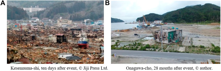
FIGURE 1. Views of disaster sites. (A) Kesennuma-shi, ten days after event, ©Jiji Press Ltd. (B) Onagawa-cho, 28 months after event, ©author.

Numerical simulations of tsunami waves acting on structures have been widely conducted since the occurrence of the 2004 Indian Ocean tsunami. For example, Shigihara et al. (2009) carried out two-dimensional and three-dimensional analyses on a bridge subjected to a tsunami wave force and confirmed that the latter model was more effective in simulating the flow paths around the bridge and evaluating the impact of the wave force acting on the bridge girder. Lau et al. (2011) conducted hydraulic experiments on a bridge model—a realistic model with piers and decks on an actual scale—measured the forces and pressures, and compared them with numerical results obtained via a commercial computational fluid dynamics program. A method to predict the maximum values of various tsunami wave forces on bridge decks was proposed. Asai et al. (2014) conducted a numerical simulation on a tsunami evacuation building model using stabilized incompressible smoothed particle hydrodynamics (SPH) and successfully verified the obtained fluid forces with those in the current design code in Japan. Furthermore, Miyagawa and Asai (2015) conducted a washout simulation of a bridge using the SPH method, in which a rigid body motion was introduced for the fluid-rigid interaction behavior. Sarfaraz and Pak (2017) also used the SPH method to evaluate tsunami-induced loads on bridge superstructures and succeeded in proposing simple design equations. In addition, several studies were conducted using simulated tsunami wave forces, and no other dynamic loads, such as seismic excitations or debris impact, were introduced. However, in reality, structures are likely to face tsunamis after being damaged by seismic excitations and could possibly experience debris collisions in a tsunami flow. Therefore, evaluations of these multi-phase loads should be considered in the design of safer tsunami evacuation buildings. In this respect, Goda et al. (2017) developed a computational framework for coupled simulation of strong motion and tsunami due to megathrust subduction earthquakes which can be used to multi-hazard risk assessments of buildings and infrastructure in the coastal region. Macabuag et al. (2018) proposed a methodology, applying several statistical techniques advanced in the field of fragility analysis, to quantify the effect of debris impact on fragility and vulnerability curve derivation using a building-by-building damage dataset obtained from the 2011 Great East Japan Earthquake and Tsunami. Carey et al. (2019) proposed a methodology to predict damage from sequential earthquake and tsunami hazards by making multihazard interaction diagrams and applied to a soil–foundation–bridge model. Petrone et al. (2020) investigated the response of a reinforced concrete frame subjected to realistic ground motion and tsunami inundation time histories to find that there was a small impact of the preceding earthquake ground shaking on the tsunami fragility. These works were mainly aiming to quantify risk assessments of structures under multi-hazard situation. However, as Carey et al. (2019) suggested, the three-dimensional effects of debris impact and more accurate calculation of hydrodynamic forces, preferably considering fluid–structure interaction effects, should be taken into account to obtain more detailed information.

This study aims to develop effective analytical tools that can comprehensively be applied to buildings under multi-phase hazardous loads such as seismic motion, fluid force, and debris impact. Simulations by two kinds of analytical tools were conducted. First, a sequential simulation of a steel frame building under seismic excitation, tsunami force, and impact force induced by debris collision was conducted using the ASI (Adaptively Shifted Integration)-Gauss code (Lynn and Isobe, 2007), which simulates behaviors of structures by simple modeling. Then, the effects of each load on the behavior of the building were investigated. The steel frame building model was first excited under a seismic acceleration observed in Kesennuma-shi during the earthquake, and then drag and buoyant forces driven by a tsunami wave were applied. Finally, the collapse behavior of the building was investigated by implementing a sophisticated contact algorithm in the numerical code to express a collision between debris and a building.

The second simulation was done by using the stabilized finite element method (FEM) (Tezduyer, 1991) based on the volume of fluid (VOF) method (Aliabadi and Tezduyar, 2000; Tanaka et al., 2012), to estimate a drag coefficient of an actual tsunami evacuation building with openings. Foster et al. (2017) proposed a set of equations for predicting forces on rectangular buildings impinged by nominally unsteady tsunami inundation flows by conducting experiments using a tsunami generator. However, it is usually very costly to obtain precise drag coefficients or forces acting on surface of a building especially when openings exist. In this study, the practicability of an estimated wave force using the drag coefficient, which was simply estimated using the inundation heights and flow velocities of tsunamis, was confirmed by comparing with the wave force obtained from the fluid analysis. Finally, a sequential simulation with a debris collision phase at the end was conducted using the ASI-Gauss code to simulate the washout behavior of the building.

To concisely describe the study, this paper is organized as follows. In Numerical Frameworks, the outline of numerical frameworks used in this paper is described. In Behavior of a Steel Frame Building Under Multi-Phase Loads, the numerical model, conditions, and results of a sequential simulation conducted on a steel frame building are introduced. The relations of the impact conditions, such as velocity, inundation height, and floating state of debris, on the surface of the building to its maximum story drift angle are discussed. In Evaluation of the Wave Force and Debris Impact Analysis of a Tsunami Evacuation Building, the results obtained from a fluid analysis are presented, and the practicability of an estimated wave force is evaluated by comparing it with a simulated one. Finally, the behavior of an actual tsunami evacuation building under debris collisions is shown. Conclusions presents the conclusions drawn from the results.

Numerical Frameworks

ASI-Gauss Code

The structural analyses in this paper were all conducted using the ASI-Gauss code utilizing linear Timoshenko beam elements (Lynn and Isobe, 2007), which can reduce memory use without losing its numerical accuracy. In this code, elasto-plastic behavior of an element is simulated appropriately, and a convergent solution is achieved with only two elements per member by shifting the numerical integration point adaptively to form a plastic hinge at exactly the point where a fully plastic section is formed.

Yielding of an element is determined by using the following equation:

where $M_x$, $M_y$, and $N$ are the bending moments around the x-axis, y-axis, and axial force, respectively, and $f_y$ is the yield function. The variables with subscript 0 are the resultant forces that form a fully plastic section in an element when they act independently on the cross section.

When the plastic hinge is determined to be unloaded, the corresponding numerical integration point is shifted back to its normal position. Here, the normal position indicates the location where the numerical integration point is placed when the element acts elastically. Generally, the normal position of the numerical integration point in linear Timoshenko beam element is midpoint, which is optimal for one-point integration. On the other hand, the normal positions of the numerical integration points are placed, in the ASI-Gauss code, at appropriate locations for two-point integration by forming a member with two elements. In this way, the stress evaluation points coincide with the Gaussian integration points of the member. It is effective to reduce inaccuracy that comes from one-point integration, evaluating low-order displacement function of the beam element.

Considerations of member fracture, elemental contact and contact release are inevitable to simulate collapse behaviors of structures. However, a precise and detailed consideration of these phenomena may lead to excessive consumption of memory resources and CPU time. In the ASI-Gauss code, some algorithms simple enough to match the rough approximations of structural members by beam elements, are adopted.

Member fracture is expressed, in this code, by reducing the sectional forces of the element immediately after the occurrence of a fractured section on either end of the element. Member fracture can be determined using bending strains, shear strains and axial tensile strains that occur in the elements, as shown in the following equation:

where ${\kappa }_x, {\kappa }_y, {\gamma }_{xz}, {\gamma }_{yz}, {\epsilon }_z$, ${\kappa }_{x0}, {\kappa }_{y0}, {\gamma }_{xz0}, {\gamma }_{yz0}$ and ${\epsilon }_{z0}$ are the bending strains around the x- and y-axes, the shear strains for the x- and y-axes, the axial tensile strain and the critical values for these strains, respectively. The critical strain values used in the analysis were obtained from experiments, performed to evaluate shear deformation behavior of high strength bolts connecting structural members (Hirashima et al., 2007). These critical values should be carefully selected and validated, if possible, because a difference in the critical values may affect the results in detail though there should be less influence in the general trends.

Contact between objects is determined in this code, first by evaluating the geometric relations of the four nodes of two beam elements in potential contact (Isobe, 2014). Once they are determined to be in contact, the elements are bound with a total of four gap elements between the nodes. The sectional forces are delivered through these gap elements to the connecting elements. To express contact release, the gap elements are automatically eliminated at the time when the mean value of the deformation of gap elements is reduced to a specified ratio.

As the extremely large rotations and strains are expected to occur in these kinds of dynamic collapse analyses, a time integration scheme based on the updated Lagrangian formulation (ULF) is used in this numerical code. The nodal displacement increment vector based upon the ULF, at step n, is expressed as follows:

where $\left\{\Delta u\right\}$is the initial nodal displacement increment vector. [⁰T] and [^uT] in Eq. 3, are the transformation matrix from global coordinates to the initial elemental coordinates and the transformation matrix from the initial elemental coordinates to elemental coordinates at step n, respectively. Here, [^uT] is calculated by successive iteration and is expressed as follows:

where [ⁿT] is the transformation matrix from elemental coordinates at step n-1 to elemental coordinates at step n. The matrix [ⁿT] is calculated as follows:

where

By defining the nodal displacement increments between step n-1 and n as ${\Delta }_{n-1}{u}_1$, ${\Delta }_{n-1}{v}_1$, ${\Delta }_{n-1}{w}_1$, $\cdots$, ${\Delta }_{n-1}{\theta }_{x2}$, ${\Delta }_{n-1}{\theta }_{y2}$ and ${\Delta }_{n-1}{\theta }_{z2}$ respectively, $\cos {(}^n\alpha )$, $\cos {(}^n\beta )$ and ${}^n\gamma$ in Eq. 6 can be calculated as follows:

where ⁿ⁻¹l is the element length at incremental step n-1.

The sectional force vector at step n+1 can be obtained by transforming the updated Kirchhoff sectional force increment vector to the Jaumann differential form vector. The strain vector and sectional force vector are thus expressed as follows:

The transformation matrix [ⁿ⁺¹A] is expressed as

where ⁿ⁺¹T*_ij is the (i, j) term of the (n+1)th matrix of Eq. 6.

The simplicities of the algorithms match the simplified approximations of structural members using beam elements, while their reliabilities were well guaranteed according to the verification and validation results (Isobe et al., 2013). These algorithms were implemented to the ASI-Gauss code, and applied to various collapse problems of structures (Isobe et al., 2012a; Isobe et al., 2012b; Javidan et al., 2018).

Stabilized FEM Based on the VOF Method

The fluid analyses in the latter part of this paper were all conducted using the stabilized FEM based on the VOF method (Tanaka et al., 2012).

To model a free surface, we consider two immiscible fluids, $\alpha$ and $\beta$, with densities ${\rho }_{\alpha }$ and ${\rho }_{\beta }$, and viscosities ${\mu }_{\alpha }$ and ${\mu }_{\beta }$. The interface function $\varphi$ serves as a marker identifying fluids $\alpha$ and $\beta$ with the definition $\varphi =\text{{}1\text{ for fluid }\alpha \text{ and 0 for fluid }\beta \text{ }}$ (Aliabadi and Tezduyar, 2000). In this paper, the density and viscosity, $\rho$ and $\mu$, are defined as

The time dependent of interface function is governed by the following advection equation:

The velocity $u$ is obtained from the solution of Navier-Stokes equations:

where $p$ is the pressure and $\mathbf{f}$ is external body force.

The stabilized finite element formulation of Eq. 14 can be written as follows:

where ${\tau }_{IC}$is the stabilization parameter.

The stabilized finite element formulation (Tezduyer, 1991) of Eqs. 15, 16 can be written as follows:

where ${\tau }_S$, ${\tau }_P$ and ${\tau }_C$ are the stabilization parameters, and $\mathbf{h}$ represents the Numann boundary condition of momentum equation.

For the temporal discretization, interface function $\varphi$, velocity $\mathbf{u}$ and pressure $p$ are discretized by using Crank-Nicolson method.

From the above discretization in space and time, a linear equation system can be obtained. GPBi-CG (Generalized product-type methods based on Bi-CG) method (Zhang, 1997) is used to solve the linear equations. In larger scale problem, this procedure takes long computational time and huge memory usage. In order to reduce them, the MPI and OpenMP hybrid parallelization is implemented.

Behavior of a Steel Frame Building Under Multi-Phase Loads

Numerical Models and Conditions

In the first part of this paper, a six-story three-span steel frame building was modeled, as shown in Figure 2, and sequential structural analyses were conducted using the ASI-Gauss code to investigate the behavior of the building under multi-phase loads. The floor height and span length were 3.6 m and 6 m, respectively. This building was designed with a base shear coefficient of 0.3. A floor load of 400 kgf/m² was applied to every floor. Subsequently, a ship fabricated out of aluminum alloy was constructed as the debris model. The ship weighed 110 tons and was 27-m long, 6-m wide, and 8-m high. It was placed at front of the building in two different types of floating states as shown. The member lists of the building and debris are shown in Tables 1, 2, respectively. These members were modeled as perfect elasto-plastic bodies with bi-linear type stress-strain relationships. The critical strain values for fracture condition given in ASI-Gauss Code, which were derived from the experiments conducted by (Hirashima et al., 2007), are shown in Table 3. These critical values were used throughout all the analyses shown in this paper.

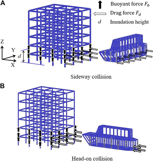
FIGURE 2. Numerical models and the buoyant and drag forces applied to the models. (A) Sideway collision. (B) Head-on collision.

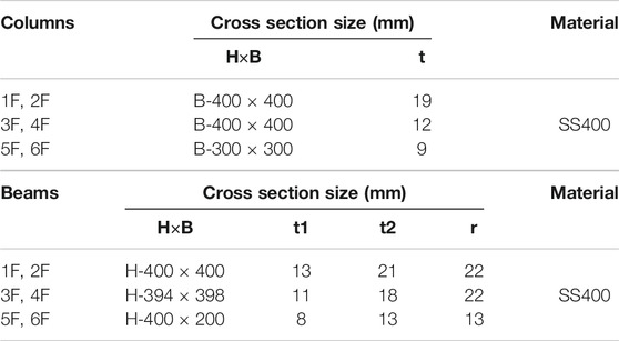
TABLE 1. Member lists of the building model.

TABLE 2. Member list of the debris model.

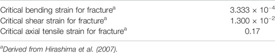
TABLE 3. Fracture condition.

The seismic record shown in Figure 3A, observed at Kesennuma-shi during the 2011 Great East Japan Earthquake, was applied to the base of the building as an input in the first phase of the simulation. It was applied for 150 s from the commencement of the seismic record.

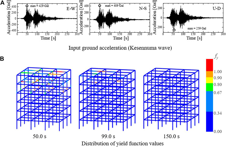
FIGURE 3. Input wave and the damage to the building. (A) Input ground acceleration (Kesennuma wave). (B) Distribution of yield function values.

Then, in the second phase of the simulation, buoyant and drag forces were applied, the former statically and the latter dynamically, at the nodes along the structural members indicated in Figure 2. The buoyant force applied to the debris balance with weight and is expressed as

where ${\rho }_s$, $g$, and $V$ are the density of sea water mixed with debris, which is 1,200 kg/m³, the acceleration of gravity, and the volume of water displaced by an object, respectively. In the case of a building model with walls under the water line (WL), the total volume of the building under the WL was used as$V$. In the case of a model without any walls under the WL, only the volume of the columns and beams under the WL was used. The drag force depends upon the relative velocity between the two objects and is calculated by

where $A, C_d, U$are the areas under the WL projected against a water flow, the drag coefficient, and the relative velocity between the two objects, respectively. A value of 1.2 was set for $C_d$ in this analysis; this value is typically used when the drag force is applied to a rectangular object. The drag force was calculated under a flow velocity of 10 m/s, which was kept constant throughout the analysis. The entire area below the WL was used as $A$ for the model with walls under the WL, and the projected area of columns and beams below the WL was used as $A$ for the model without walls under the WL. For example, the total drag force acting on the front surface of the model with walls was calculated to be 7.8 MN, whereas the force on the model without walls was 0.7 MN when the flow velocity and inundation height were set to 10 m/s and 6 m, respectively.

In the final phase of the simulation, the debris model was collided with the building model by applying the same velocity as the tsunami flow. Initially, the relative velocity between the tsunami flow and the debris was 0 m/s, and thus, the value of the drag force applied to the debris was 0 MN. On impact, the value increased to 3.3 MN in case of the sideway type collision (Figure 2A), if the motion of the debris was completely stopped. The time increment of the dynamic analysis was 1 ms, which was numerically solved by Newmark’s β method considering numerical damping (β = 4/9, δ = 5/6) (Press et al., 1992).

Numerical Results

Figure 3B shows the damage to the building under the Kesennuma wave at the moment when the yield function values of Eq. 1 reached their maximum values. They reached their maximum in some beams and columns at the first peak of the seismic motion around 50 s; however, the seismic excitation seems to have caused no significant damage to the building.

Figure 4A shows the damage of the model with walls under the WL, under the tsunami flow and sideway type debris collision, simulated in the following phases. An extremely large drag force was applied to the walls by the tsunami flow, nearly causing critical damage to the entire building. The building withstood the tsunami flow; however, it was finally washed away by a critical blow provided by the debris collision. After the impact, the debris became integrated and moved with the building until it reached the same velocity as the tsunami flow itself. Eventually, the drag forces of the building and debris decreased to 0 MN (Figure 4B) as the relative velocity between them decreased (Figure 4C).

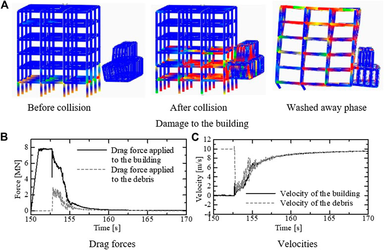
FIGURE 4. Numerical results for the model with walls under WL. (A) Damage to the building. (B) Drag forces. (C) Velocities.

Figure 5A shows the damage of the model without walls under the WL, under the tsunami flow and the same type debris collision. Because there were no walls under the WL, the building endured the fluid force during the second phase. As shown in Figure 5B, the drag force applied to the building became smaller than half that applied to the debris after the collision. Concurrently, the drag force applied to the debris became larger than the value in Figure 4B because the relative velocity remained large as the building maintained its stance after the collision and did not wash away. Although the debris was torn apart after the impact, some parts of the debris and the building remained intact, and their velocities both became 0 m/s in the tsunami flow (Figure 5C).

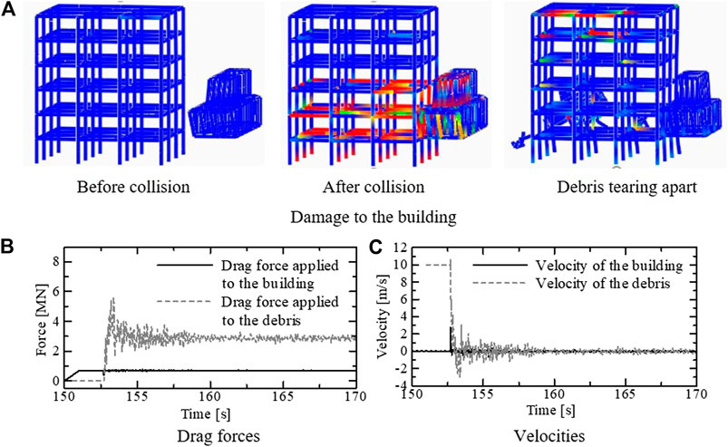
FIGURE 5. Numerical results for the model without walls under WL. (A) Damage to the building. (B) Drag forces. (C) Velocities.

Next, impact analyses under the head-on collision shown in Figure 2B were conducted and the results were compared between the two types of collisions. In the head-on collision cases, the drag force acting on the debris is reduced because the projected area is smaller, whereas the impact force applied to the building may intensify. Figure 6 shows the deformation of the building at different inundation heights and types of collision for the model with and without walls under the WL. The broken line in the figure shows the story drift angle of severely damaged steel frame Rahmen structures, 1/40, as determined by the Tokyo Association of Architectural Firms, Japan (TAAF, 2019). As shown in Figure 6A, every maximum story drift angle of the building in head-on collision cases is larger than that in the sideway collision cases when the inundation height is lower (d = 3 m and d = 4 m). The same tendency can be observed in Figure 6B for the model without walls under the WL, but smaller in values in most cases compared to those in Figure 6A. Figure 7 shows the distribution of yielded columns, which were evaluated using Eq. 1, and a description of relations between the debris state and the local damage. As depicted in Figure 7A, the columns at the lower levels are severely damaged by the concentrated impact force on the lower levels of the building, which leads to an increase in the maximum story drift angle. In contrast, there are some cases with higher inundation heights (d = 5 m and d = 6 m in Figure 6), in which the building is more severely damaged if the debris hits sideways and at higher velocities. As depicted in Figure 7B, this is caused by a large drag force acting on the debris facing sideways, distributing a large lateral force to the intact building in a high-speed tsunami flow. In summary, the damage to the building intensifies if a head-on collision occurs under a tsunami flow with a lower inundation height, and the damage to the building becomes larger if sideway collisions occur under a tsunami flow with a higher inundation height and higher velocity.

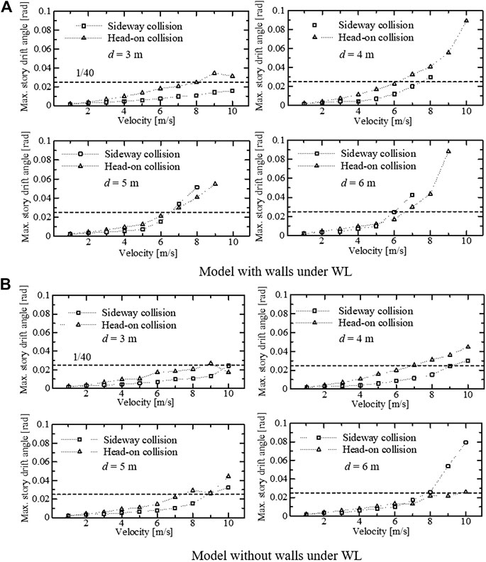
FIGURE 6. Deformation of the building in different inundation heights and types of collisions. (A) Model with walls under WL. (B). Model without walls under WL.

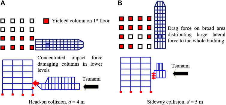
FIGURE 7. Difference between the types of collisions and the cause of damage in lower levels (model with walls under WL). (A) Head-on collision, d = 4 m. (B) Sideway collision, d = 5 m.

Evaluation of the Wave Force and Debris Impact Analysis of a Tsunami Evacuation Building

In the second part of this paper, the outcomes of a one-way coupling analysis of a tsunami evacuation building, which was designed for actual use, are discussed. Three-dimensional free surface flow analysis was carried out using the stabilized FEM (Tanaka et al., 2012) based on the VOF method to obtain the time history of wave force applied to the building. By using this result, the drag coefficient of the building that appear in the empirical Eq. 20 would be estimated. The numerical code has been fully verified and validated by solving various types of benchmark problems and by comparing the results with an experiment of concrete material under an impulsive tsunami loading conducted in a large-scale testing flume at the Port and Airport Research Institute, Japan (Arikawa, 2009).

Computation of the Wave Force Using the Stabilized FEM

A 240-m long, 180-m wide, and 80-m high numerical model, as shown in Figure 8, was constructed for the fluid analysis. The building model located at the center is a 40.15-m high and 32.00-m wide 10-story building with openings. The reduction coefficient $\gamma$ of this building can be calculated as 0.52 when the inundation height is 8.0 m. Here, $\gamma$ is defined as the ratio of the projected area of the walls to the entire area under the WL (MLIT, 2011). This building is shown as a design example in the practical guide published by NILIM (2012). The model was subdivided with tetrahedron elements that did not allow deformations, and the distances between nodes were set close to 0.5 m under the WL and around the building. The total numbers of nodes and elements were approximately 3.7 million and 21 million, respectively.

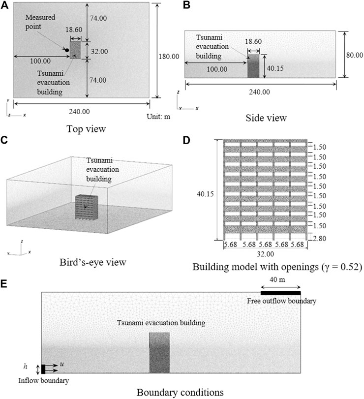
FIGURE 8. Dimensions of the numerical model and boundary conditions for fluid analysis. (A) Top view. (B) Side view. (C) Bird’s-eye view. (D) Building model with openings (γ = 0.52). (E) Boundary conditions.

The boundary condition of the fluid analysis is shown in Figure 8E. An inflow boundary was set at the lower left corner, where seawater flowed into the area. An outflow boundary was set at the upper right corner, where air flowed out freely without traction. Furthermore, a slip condition was assumed for other areas between the fluid and the wall surface. A case with an upstream depth of 8.0 m and flow velocity of 12 m/s was simulated. Here, the upstream depth is defined as the inundation height at a location distant from the building. The densities of seawater and air were 1,027 kg/m³ and 1.293 kg/m³, and the viscosity coefficients of seawater and air were 1.0 × 10⁻³ Pa･s and 1.8 × 10⁻⁵ Pa･s, respectively. The time increment was 0.01 s, and a total duration of 30 s was simulated. The computational time was approximately 24 h when using 96 parallel processors (8 nodes × 12 processors) of PC cluster parallel computers (3.33-GHz CPU, 48-GB RAM).

Figure 9 shows the overall view and pressure distribution calculated at the front surface of the building. The tsunami wave flows in and propagates until it collides with the front surface of the building. The wave heights of the free surface are amplified by short, reflected waves, and appear to be well simulated. In addition, seawater flowing in and out of the openings can be observed. A wide area of the building under the WL is pressurized; however, the pressure does not become much higher as it was expected, because seawater flows into the building through the openings.

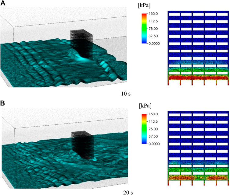
FIGURE 9. Overall view (left) and pressure distribution at front surface of the building (right). (A) 10 s (B) 20 s.

Evaluation of the Estimated Wave Force

Next, an estimated wave force, which can be simply calculated from the inundation heights and flow velocities, is compared with the simulated wave force obtained from the fluid analysis. Here, the sum of the hydrostatic load $F_s$ and drag force $F_d$ is defined as the estimated wave force by assuming that only a stationary force dependent on the inundation height and fluid velocity acts on a building. The former and latter forces are distributed in triangular and rectangular shapes, respectively, on the surface of the building, as shown in Figure 10. These forces are expressed by the following equations using the above-mentioned reduction coefficient $\gamma$ (MLIT, 2011) to consider the reduction in the wave force owing to openings:

where $B$ is the width of the pressurized surface, $z_1$ and $z_2$ are the minimum and maximum heights of the pressurized surface, respectively, and $h$ is the inundation height.

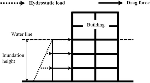
FIGURE 10. Hydrostatic load and drag force acting on the surface of the building.

The estimated wave force calculated using Eqs 21, 22 was compared with the simulated wave force obtained from the fluid analysis described in Computation of the Wave Force Using the Stabilized FEM. Here, the drag coefficient $C_d$ was calibrated by a numerical simulation with a rectangular-shaped building model with openings and was set to 1.5 (Tanaka and Isobe, 2018). Figure 11 shows a comparison between the estimated and simulated forces in the case of γ = 0.52. The time history of the former was obtained by applying a hydrostatic load in one step and by incrementally applying a drag force for 1 s till it reached to a specific value calculated using Eqs 21, 22. As shown in the figure, the estimated wave force roughly approximates the stationary component and is in compliance with the simulated wave force.

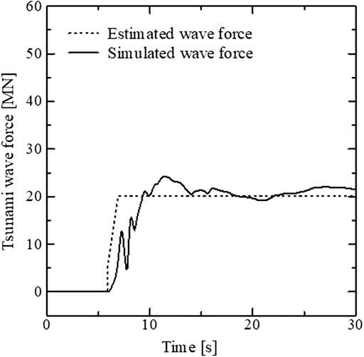
FIGURE 11. Comparison between estimated and simulated wave forces (γ = 0.52).

The computational cost of three-dimensional fluid analysis will become high, especially if we consider various wave conditions. Once we simulate a three-dimensional fluid analysis and estimate the drag coefficient of the building that has arbitrary shapes, significant reduction of computational cost to estimate the wave force in various conditions should be achieved.

Numerical Models for the Debris Impact Analysis

A sequential simulation using the estimated wave force, with a debris collision phase at the end, was conducted using the ASI-Gauss code (Lynn and Isobe, 2007) to simulate the washout behavior of a building. The numerical models used for the analysis are shown in Figure 12. The columns, beams, floors, foundation beams, and piles of the building were all modeled with linear Timoshenko beam elements. As described earlier, the building was a 40.15-m high, 32.00-m wide, 10-story steel-framed building, designed under a base shear coefficient of 0.16. The floor heights were 3.95 m, excluding the 1st floor with a height of 4.60 m. The damping ratio was set to 2%. The cross-section sizes of columns and beams used in the building are shown in Tables 4, 5, respectively. The specifications of the structural members were as follows: columns (square steel pipes, BCP325), girders (H-type steel beams, SN490B), and binders (H-type steel beams, SN490B). Basically, these members were modeled as perfect elasto-plastic bodies with bi-linear type stress-strain relationships. The material parameters of SN490B were as follows: Young’s modulus 205 GPa, Poisson’s ratio 0.3, yield stress 325 MPa, and density 7.85 × 10⁻⁶ kg/mm³. The concrete piles were 30 m in length with a 2-m-wide circular section, each with a weight of 1.32 MN; however, they were approximated by replacing them with 3-m-long piles with square sections of the same area, having the same strength. The floors, piles, and foundation beams were all modeled with elastic elements. The floor loads were 540 kgf/m² on the 1^st to 10th floors and 670 kgf/m² on the roof. Nonstructural components were not modeled; however, the weights were added to the elements constituting the beams and floors by incorporating into their densities. The total weight of the building, which was 58.90 MN, showed the same value as in (NILIM, 2012). The natural periods, which were 1.36 s in the X-direction and 1.37 s in the Y-direction, and the ultimate horizontal resistant forces of the model also demonstrated compliance with the values in the reference. The total numbers of elements and nodes were 3,720 and 2,350, respectively.

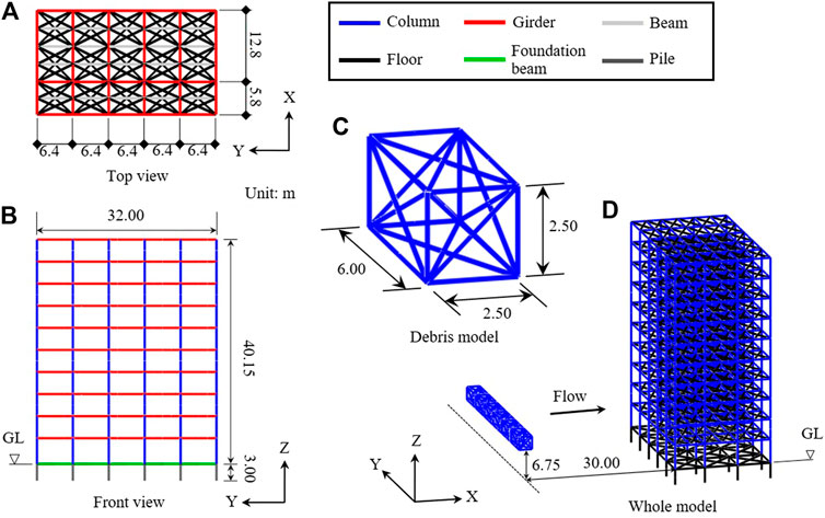
FIGURE 12. Dimensions of the tsunami evacuation building and debrits.

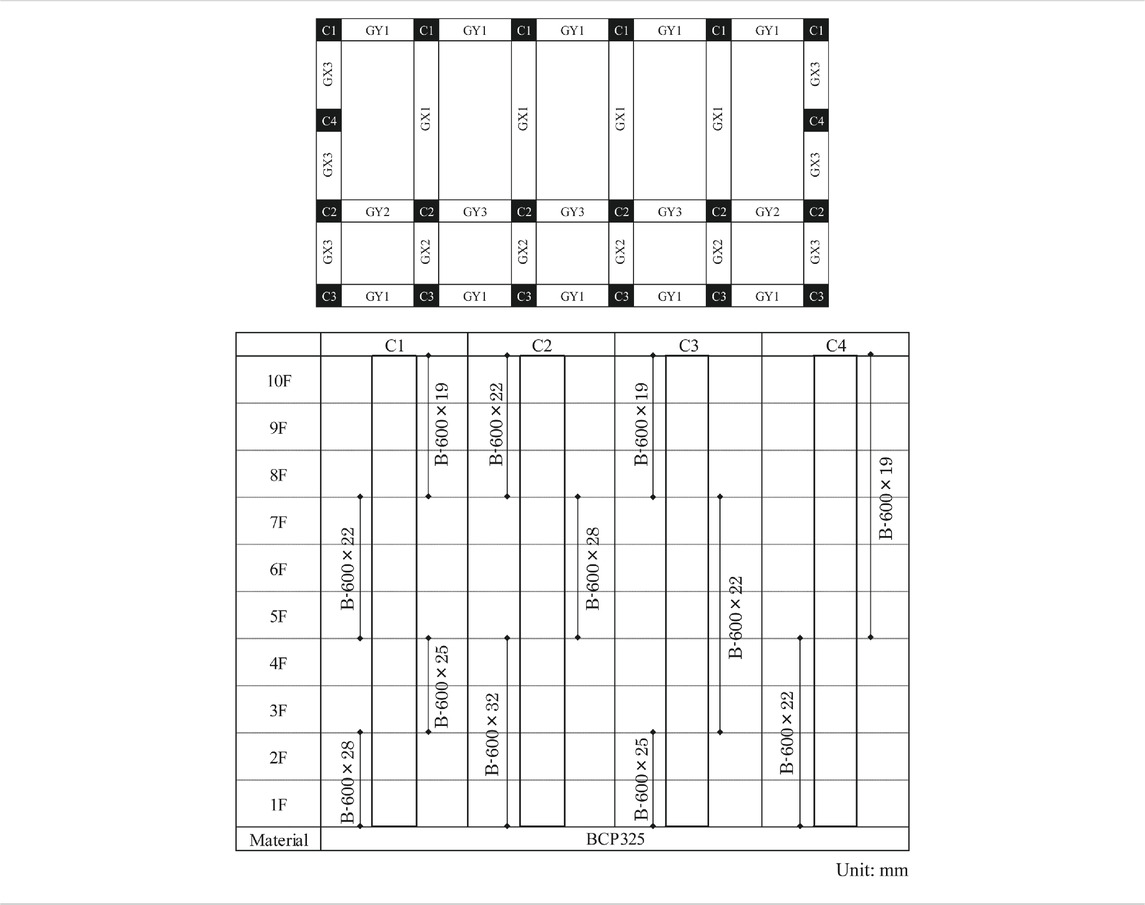
TABLE 4. Cross section sizes of columns used in the building.

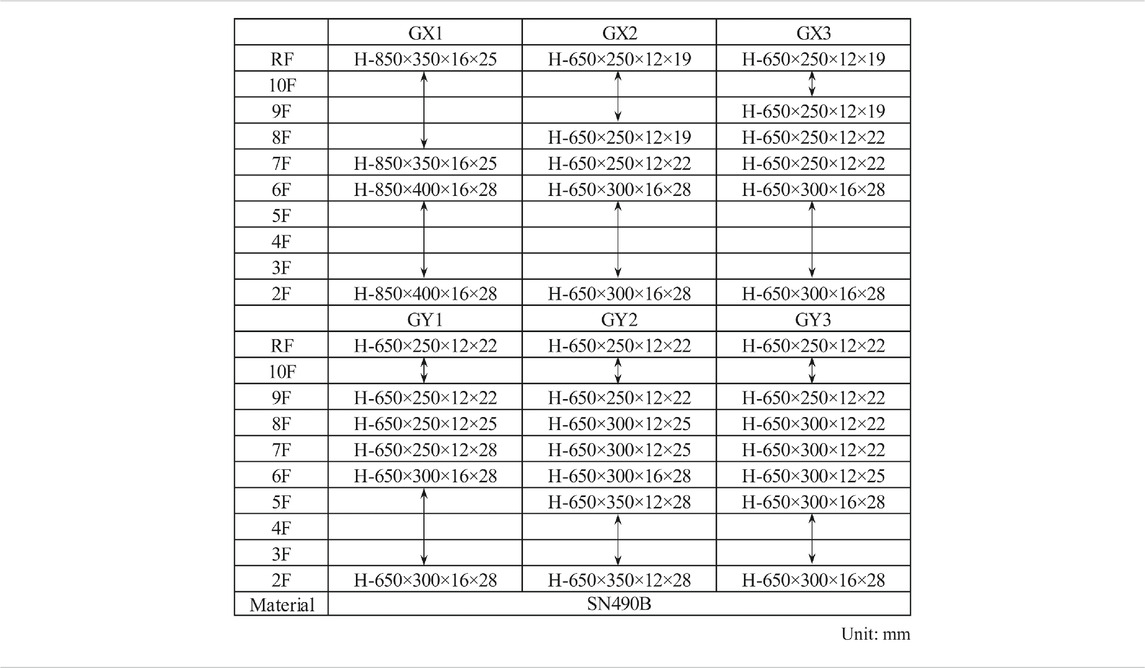
TABLE 5. Cross section sizes of beams used in the building.

As also shown in Figure 12, a 6.0-m long, 2.5-m wide, and 2.5-m high container box made of SS400 steel weighing 24.0 t was constructed as the debris model. Six of these container boxes, with drafts of 1.25 m, were connected side by side and placed 30.0 m away from the front surface of the building.

Load Conditions

A three-dimensional K-NET Sendai wave observed during the 2011 Great East Japan Earthquake, as shown in Figure 13A, was used as the input ground acceleration. As can be seen in the acceleration response spectrum (Figure 13B), the predominant periods of the K-NET Sendai wave were 0.65 s in the east-west (E-W) and north-south (N-S) directions, and 0.15 s in the up-down (U-D) direction. A part of the seismic record, including two peaks, from t = 0 s to t = 150 s was applied in the analysis.

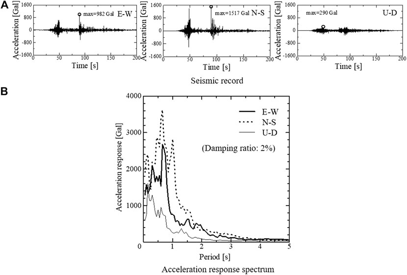
FIGURE 13. Input ground acceleration (K-NET Sendai wave). (A) Seismic record. (B) Acceleration response spectrum.

Then, the forces induced by the tsunami wave were applied to the building model. Among these forces, the buoyant force $F_b$ acting vertically upward on the building under the WL was calculated using Eq. 19. The estimated wave force evaluated in the previous section, calculated under a flow velocity of 12 m/s, was used as the horizontal force applied to the building with openings (γ = 0.52). This force was applied to the nodes along the structural members on the front surface of the model under the WL. Both the hydrostatic load and buoyant force were applied statically in one step, and the drag force was applied dynamically for 1 s in the following steps till it reached to a specific value calculated using Eqs 21, 22.

In the final phase of the sequential simulation, only a drag force was applied to the boxes, and they were moved toward the building with the same velocity as the tsunami flow to simulate the impact phenomena.

Numerical Results

The behavior of the building under the K-NET Sendai wave is shown in Figure 14A. The elements are classified by colors according to the yield function values $f_y$ as in the previous section. As shown, the building deforms considerably, and comparatively large sectional forces appear at the first peak (t = 46.0 s) and at the second peak (t = 90.5 s) of the input wave. Figure 14B shows the residual and maximum interstory drift angles. The maximum interstory drift angle was observed at the seventh floor and reached nearly 1/50 rad. The angles were only 1/100 rad or greater at other floors. However, the residual interstory drift angle presented a maximum value of only 1/400 rad on the third floor; hence, the building could be evaluated as almost undamaged from this standpoint.

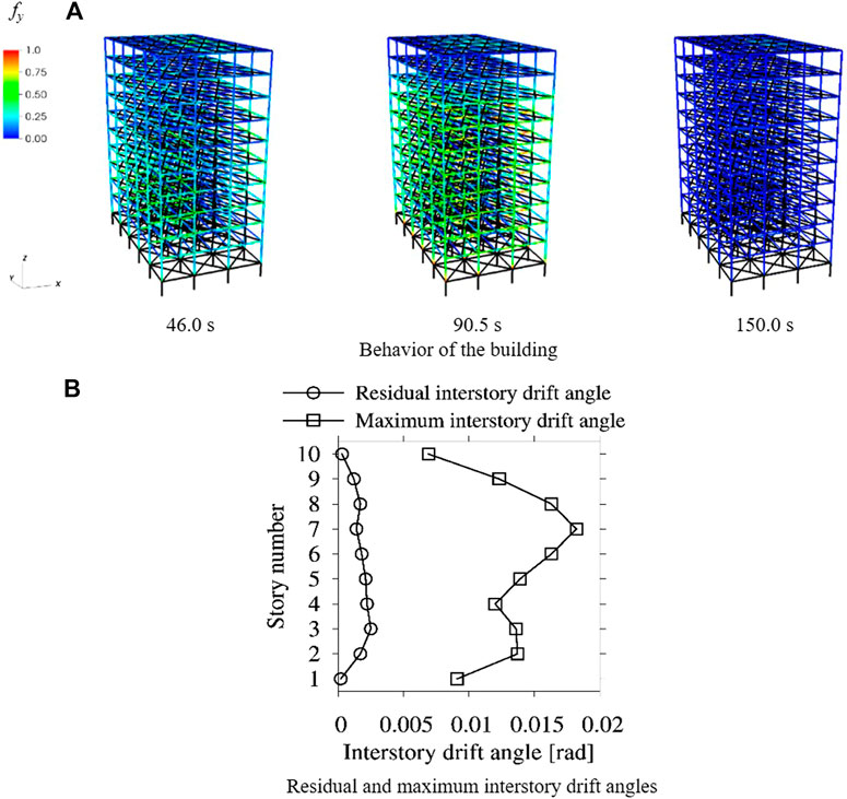
FIGURE 14. Damage of the building under K-NET Sendai wave. (A) Behavior of the building. (B) Residual and maximum interstory drift angels.

The application of the estimated wave force, calculated under the selected conditions, did not cause severe damage to the building. However, collisions with the container boxes that followed the application of the tsunami wave force caused obvious damage to the building. Figure 15 shows the behavior of the building during the debris collision. Material failures of columns and beams can be observed as the container boxes make their contact near the beam–column joint sections of the second and third floors. A shock wave runs rapidly through the building from the impact point. As the debris collides and its velocity is reduced at the front of the building, the relative velocity between the tsunami flow and debris increases. Inevitably, the debris and building are subjected to a considerably larger drag force. Member fractures first occur at the front columns of the first floor, and the destruction propagates progressively to the inside. Finally, the building collapses and is washed away.

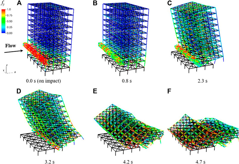
FIGURE 15. Behavior of the building due to application of estimated wave force and impact of tsunami debrits. (A) 0.0 s (on impact). (B) 0.8 s (C) 2.3 s (D) 3.2 s (E) 4.2 s (F) 4.7 s.

Conclusions

This study aimed to develop effective analytical tools that can comprehensively be applied to buildings under multi-phase hazardous loads such as seismic motion, fluid force, and debris impact. Simulations by two kinds of analytical tools were conducted. First, a sequential simulation of a steel frame building under seismic excitation, tsunami force, and impact force induced by debris collision was conducted using the ASI-Gauss code, which simulates behaviors of structures by simple modeling. The second simulation was conducted by using the stabilized FEM based on the VOF method, to estimate a drag coefficient of an actual tsunami evacuation building with openings. A debris collision phase at the final phase was conducted using the ASI-Gauss code to simulate the washout behavior of the building. The key findings of this study are summarized as follows:

1. A structural analysis of a common, six-story three-span steel frame building subjected to the seismic record, observed at Kesennuma-shi during the 2011 Great East Japan Earthquake, showed no significant damage to the building.

2. It became evident that the damage to the building intensifies if a head-on collision occurs under a tsunami flow with a lower inundation height, and the damage to the building becomes larger if sideway collisions occur under a tsunami flow with a higher inundation height and higher velocity.

3. The stabilized FEM based on the VOF method had well simulated the overall tsunami flow including the pressure distribution at the front surface of the building. Phenomena such as flowing in and out of the openings, and amplification of short, reflected waves were well simulated. It was confirmed that the pressure under the WL did not become much higher as it was expected, because seawater flowed into the building through the openings. Also, the drag coefficient of the building with arbitrary shape that appears in the empirical equation of wave force was well estimated.

4. The estimated wave force calculated using inundation heights and flow velocities matched well with the simulated wave force obtained from the fluid analysis. However, the former does not replicate the impulsive components in wave forces, and the disadvantages of using a simple estimated value should be noted.

5. As shown in both simulations, the ASI-Gauss code has practically simulated the impact phenomena of debris and damage to buildings. However, the flow channel geometry may change according to the current directions near the openings. A more precise flow path for tsunami debris near the buildings should be considered in future investigations.

It is well worth noting that the three-dimensional effects of debris impact and more accurate calculation of hydrodynamic forces, preferably considering fluid–structure interaction effects, should be taken into account to obtain more detailed information. Then, risk assessments of structures under multi-hazard situation could be quantified more accurately. In this respect, a more advanced coupling analysis for fluid–structure interaction is urgently needed.

Data Availability Statement

The raw data supporting the conclusions of this article will be made available by the authors, without undue reservation.

Author Contributions

DI mainly organized this work and has written the whole paper. ST conducted most of the analysis in this paper.

Funding

This work was supported by JSPS KAKENHI Grant Number JP17H02057.

Conflict of Interest

The authors declare that the research was conducted in the absence of any commercial or financial relationships that could be construed as a potential conflict of interest.

Acknowledgments

The authors would like to acknowledge the contributions of Mr. Yuan Qi Dong of Japan-China Consultant Co., Ltd. and Mr. Hiroaki Ogino of JFE Engineering Co., former graduate students of the University of Tsukuba.

References

Aliabadi, S., and Tezduyar, T. E. (2000). Stabilized-finite-element/interface-capturing Technique for Parallel Computation of Unsteady Flows with Interfaces. Comp. Methods Appl. Mech. Eng. 190, 243–261. doi:10.1016/s0045-7825(00)00200-0
Arikawa, T. (2009). Structural Behavior under Impulsive Tsunami Loading. J. Disaster Res. 4 (6), 377–381. doi:10.20965/jdr.2009.p0377
Asai, M., Goda, T., Oguni, K., Isobe, D., Kashiyama, K., and Isshiki, M. (2014). Evaluation of Tsunami Fluid Force Acted on Tsunami Refuge Building by Using a Stabilized ISPH. J. Jsce 70 (2), 649. (in Japanese). doi:10.2208/jscejam.70.i_649
Carey, T. J., Mason, H. B., Barbosa, A. R., and Scott, M. H. (2019). Multihazard Earthquake and Tsunami Effects on Soil-Foundation-Bridge Systems. J. Bridge Eng. 24 (4), 04019004. doi:10.1061/(asce)be.1943-5592.0001353
Foster, A. S. J., Rossetto, T., and Allsop, W. (2017). An Experimentally Validated Approach for Evaluating Tsunami Inundation Forces on Rectangular Buildings. Coastal Eng. 128, 44–57. doi:10.1016/j.coastaleng.2017.07.006
Goda, K., Petrone, C., De Risi, R., and Rossetto, T. (2017). Stochastic Coupled Simulation of Strong Motion and Tsunami for the 2011 Tohoku, Japan Earthquake. Stoch Environ. Res. Risk Assess. 31, 2337–2355. doi:10.1007/s00477-016-1352-1
Hirashima, T., Hamada, N., Ozaki, F., Ave, T., and Uesugi, H. (2007). Experimental Study on Shear Deformation Behavior of High Strength Bolts at Elevated Temperature. Nihon Kenchiku Gakkai Kozokei Ronbunshu 72, 175–180. in Japanese. doi:10.3130/aijs.72.175_2
Isobe, D. (2014). An Analysis Code and a Planning Tool Based on a Key Element Index for Controlled Explosive Demolition. Int. J. High-Rise Buildings 3 (4), 243–254.
Isobe, D., Han, W. S., and Miyamura, T. (2013). Verification and Validation of a Seismic Response Analysis Code for Framed Structures Using the ASI-Gauss Technique. Earthquake Engng Struct. Dyn. 42 (12), 1767–1784. doi:10.1002/eqe.2297
Isobe, D., Ohta, T., Inoue, T., and Matsueda, F. (2012b). Seismic Pounding and Collapse Behavior of Neighboring Buildings with Different Natural Periods. Ns 04 (8A), 686–693. doi:10.4236/ns.2012.428090
Isobe, D., Thanh, L. T. T., and Sasaki, Z. (2012a). Numerical Simulations on the Collapse Behaviors of High-Rise Towers. Int. J. Protective Structures 3 (1), 1–19. doi:10.1260/2041-4196.3.1.1
Javidan, M. M., Kang, H., Isobe, D., and Kim, J. (2018). Computationally Efficient Framework for Probabilistic Collapse Analysis of Structures under Extreme Actions. Eng. Structures 172, 440–452. doi:10.1016/j.engstruct.2018.06.022
Lau, T. L., Ohmachi, T., Inoue, S., and Lukkunaprasit, P. (2011). Experimental and Numerical Modeling of Tsunami Force on Bridge Decks, Tsunami A Growing Disaster. Editor M. Mokhtari (London, UK): IntechOpen), 105–130.
Lynn, K. M., and Isobe, D. (2007). Finite Element Code for Impact Collapse Problems of Framed Structures. Int. J. Numer. Meth. Engng 69 (12), 2538–2563. doi:10.1002/nme.1858
Macabuag, J., Rossetto, T., Ioannou, I., and Eames, I. (2018). Investigation of the Effect of Debris-Induced Damage for Constructing Tsunami Fragility Curves for Buildings. Geosciences 8 (4), 117. doi:10.3390/geosciences8040117
Miyagawa, Y., and Asai, M. (2015). Multi-Scale Bridge Wash Out Simulation during Tsunami by Using a Particle Method. Melaka, Malaysia: MATEC Web of Conferences, 1–7.
MLIT (2011). Provisional Guideline on Requirement for Structural Design of Tsunami Evacuation Buildings Based on Building Damage Owing to Tsunami Following the 2011 off the Pacific Coast of Tohoku Earthquake. (Japan: Housing Bureau, Ministry of Land, Infrastructure, Transport and Tourism). (in Japanese).
NILIM (2012). Practical Guide on Requirement for Structural Design of Tsunami Evacuation Buildings, Technical Note of National Institute for Land and Infrastructure Management. (Japan: National Institute for Land and Infrastructure Management). (in Japanese).
NILIM (2011). “Report on Field Surveys and Subsequent Investigations of Building Damage Following the 2011 off the Pacific Coast of Tohoku Earthquake,” in Technical Note of National Institute for Land and Infrastructure Management (Japan: National Institute for Land and Infrastructure Management), 132. (in Japanese).
PARI (2011). Technical Note of the Port and Airport Research Institute. An Investigation Report on the Seismic and Tsunami Damages of Port, Coast and Airport Due to 2011 Great East-Japan Earthquake. (Japan: Port and Airport Research Institute). (in Japanese).
Petrone, C., Rossetto, T., Baiguera, M., la Barra Bustamante, C. D., and Ioannou, I. (2020). Fragility Functions for a Reinforced Concrete Structure Subjected to Earthquake and Tsunami in Sequence. Eng. Structures 205, 110120. doi:10.1016/j.engstruct.2019.110120
Press, W. H., Teukolsky, S. A., Vetterling, W. T., and Flannery, B. P. (1992). Numerical Recipes in FORTRAN: The Art of Scientific Computing. New York: Cambridge University Press.
Sarfaraz, M., and Pak, A. (2017). SPH Numerical Simulation of Tsunami Wave Forces Impinged on Bridge Superstructures. Coastal Eng. 121, 145–157. doi:10.1016/j.coastaleng.2016.12.005
Shigihara, Y., Fujima, K., and Shoji, G. (2009). Numerical Simulation of Tsunami Force Acting on the Bridge. J. Jsce, Ser. A1 65 (1), 899–904. (in Japanese). doi:10.2208/jscejseee.65.899
TAAF (2019). Recommendation for Design of Buildings 2019. (Japan: Tokyo Association of Architectural Firms). (in Japanese).
Tanaka, S., and Isobe, D. (2018). Development of Finite Element Analysis Method for Damage Estimation of Tsunami Evacuation Building. Trans. JSCES 2018 (2), 20182008. doi:10.11421/jsces.2018.20182008 (in Japanese).
Tanaka, S., Sun, F., Hori, M., Ichimura, T., and Wijerathne, M. L. L. (2012). Large-scale Failure Analysis of Reinforced Concrete Structure by Tsunami Wave Force. 15th World Conference in Earthquake Engineering (15WCEE). Lisbon: Portugal.
Tezduyar, T. E. (1991). Stabilized Finite Element Formulations for Incompressible Flow Computations. Adv. Appl. Mech. 28, 1–44. doi:10.1016/s0065-2156(08)70153-4
Keywords: sequential simulation, structural analysis, fluid analysis, steel frame building, multi-phase load, earthquake, tsunami, asi-gauss code
Citation: Isobe D and Tanaka S (2021) Sequential Simulations of Steel Frame Buildings Under Multi-Phase Hazardous Loads During Earthquake and Tsunami. Front. Built Environ. 7:669601. doi: 10.3389/fbuil.2021.669601
Received: 19 February 2021; Accepted: 19 April 2021;
Published: 07 May 2021.
Edited by:
Carmine Galasso, University College London, United KingdomReviewed by:
Marco Baiguera, University of Southampton, United KingdomIman Hajirasouliha, The University of Sheffield, United Kingdom
Copyright © 2021 Isobe and Tanaka. This is an open-access article distributed under the terms of the Creative Commons Attribution License (CC BY). The use, distribution or reproduction in other forums is permitted, provided the original author(s) and the copyright owner(s) are credited and that the original publication in this journal is cited, in accordance with accepted academic practice. No use, distribution or reproduction is permitted which does not comply with these terms.
*Correspondence: Daigoro Isobe, isobe@kz.tsukuba.ac.jp