Optimization of Condition-Based Maintenance of Wood Utility Pole Network Subjected to Hurricane Hazard and Climate Change
 Abdullahi M. Salman
 Babak Salarieh
 Emilio Bastidas-Arteaga
 Yue Li3
- 1Department of Civil & Environmental Engineering, The University of Alabama in Huntsville, Huntsville, AL, United States
- 2Université de Nantes, GeM, Institute for Research in Civil and Mechanical Engineering, CNRS UMR 6183, Nantes, France
- 3Department of Civil Engineering, Case Western Reserve University, Cleveland, OH, United States
Electric power distribution systems that link the bulk power grid (generation and transmission systems) to customers are the leading cause of power outages due to their vulnerability to extreme wind events, especially hurricanes. The strength of the wood poles that typically support the distribution lines also deteriorate over time. The vulnerability of the poles is expected to increase due to the potential impact of climate change on both hurricane hazard and wood decay rate. As such, an effective maintenance planning method is required for the vast number of poles supporting distribution lines. This paper presents a framework to optimize the maintenance of a network of wood utility poles. Corrective replacement due to failure caused by hurricanes and preventive replacement due to excessive decay are considered. The objective is to find the optimal inspection interval for the preventive replacement to minimize the long-term maintenance cost. To solve the optimization problem, the decay of the poles is modeled as a stationary gamma process. The impact of climate change on the rate of pole failure and replacement is also investigated. Two locations are considered as case studies: Miami, Florida, and New York City, New York. The period from 2010 to 2099 is considered for the study. The results of the case study show that the optimal inspection/replacement cycle determined using the developed framework results in lower total maintenance costs compared to current typical utility practice. Based on the inspection and replacement costs used in the study, the results show that adopting a periodic preventive maintenance policy decreases the failure rate of the poles but increases the total maintenance cost. However, only the cost of replacing the poles is considered here. Other considerations, such as indirect costs due to power outages and the impact of pole failure on system reliability, can render the adoption of a preventive replacement policy cost-effective. The results also show that climate change can increase the total maintenance cost. Based on current typical utility maintenance practice, climate change can increase the total maintenance cost by up to 8% in Miami and 6% in NYC, depending on the emission scenario considered.
Introduction
Electric power systems are the backbone of the complex network of infrastructure systems that support modern societies. Most civil infrastructure systems such as water and wastewater systems, transportation systems, gas supply networks, and communications systems cannot function properly without reliable power supply. Electric power systems are subdivided into generation, transmission, and distribution subsystems. The transmission system transport bulk power through high voltage conductors supported by steel lattice towers, H-frame towers, or single poles, which can be wood, steel, or concrete. The distribution system is the downstream part of the system that transports power to the customers. It is usually composed of low voltage conductors supported by single-pole structures. The majority of the poles supporting distribution systems in the U.S. and other countries are wood poles (Mankowski et al., 2002; Nguyen et al., 2004). For example, there are between 160 and 180 million wood poles in the U.S. worth billions of dollars (Mankowski et al., 2002). Similarly, around 5 million of the estimated 7 million utility poles in Australia are wood poles with a net worth of over $10 billion (Yeates and Crews, 2000; Nguyen et al., 2004). Wood poles are preferred over other materials because they are relatively cheaper to purchase, lighter and easier to transport, and are easy to climb and are non-conductive, which makes them safer for utility workers (Mankowski et al., 2002).
Wood poles are susceptible to decay over time, which leads to a decrease in strength. As such, utility companies carry out periodic maintenance on poles and replace poles with significant decay. The decay of wood poles depends on material properties, soil properties, and local climatic conditions. The main climate parameters that affect the decay of wood are humidity and temperature (Wang and Wang, 2012; Bastidas-Arteaga et al., 2015; Teodorescu et al., 2017). The exposure of wood poles to a humid environment increases the moisture content of the wood. The increase in the moisture content of wood above the fiber saturation point will provide a viable environment for the establishment of a fungal mycelial mat and further fungal growth (Viitanen and Ritschkoff, 1991). Moisture content above the fiber saturation point results in the availability of free water in the wood, which is easily accessible to the fungi and leads to rapid decay (Wang and Wang, 2012). The growth of decay fungi is also significantly affected by air and wood temperature. Generally, a temperature in the range of 5° to 65°C is considered favorable for fungal growth (Brischke and Rapp, 2008; Wang and Wang, 2012). It is, therefore, clear that the long-term performance of wood poles will be affected by any potential future climate variations.
The fifth assessment report of the intergovernmental panel on climate change (IPCC) reported that the atmospheric concentration of CO2 in 2011 exceeded the pre-industrial level by about 40% and also noted that almost the entire globe had experienced surface warming between 1901 and 2012 (IPCC, 2013). The IPCC also noted an increase in air specific humidity since the 1970s, which has abated in recent years (IPCC, 2013). However, local variations exist in the trend of both temperature and humidity changes. For example, De Larrard et al. (2014) considered the yearly changes in temperature and relative humidity (RH) for the cities of Nantes, Paris, Strasbourg, Clermont-Ferrand, Toulouse and Marseille (France) under three carbon-emission scenarios. They noted that all the emission scenarios considered resulted in an increase in temperature and a decrease in RH between 2001 and 2100 and that the impact is very different depending on the location. Peng and Stewart (2014) used six general circulation models (GCMs) to predict changes in temperature and RH for Sydney (Australia) and Kunming (China) based on two carbon emission scenarios. They found that while the six models projected temperatures to increase, relative humidity remained largely unchanged between 2010 and 2100 in both cities.
The decay of wood poles can significantly impact their ability to resist weather-related loads, such as hurricane winds. Hurricanes can cause extensive damage to power distribution systems, and recent hurricanes have demonstrated that the build and rebuild approach used by many utility companies is not viable. For example, Hurricane Rita (2005) led to the failure of over 10,000 distribution poles in Texas costing utilities over $400 million (Quanta-Technology, 2009). Similarly, over 15,000 distribution poles were damaged by Hurricane Ike in 2008 in Texas (Quanta-Technology, 2009). Elsewhere, Hurricane Andrew damaged more than 10% of all exposed distribution poles in Florida in 1999. While current design guidelines require wood poles to be designed to resist a certain level of hurricane wind, the time-dependent decrease in strength due to decay is usually not considered in the design. As such, a risk mitigation strategy for hurricane-related damages that consider the impact of decay is needed.
Future hurricane pattern is expected to be affected by climate change. The IPCC projected that the intensity of storms is expected to rise in the coming years (IPCC, 2013). Bender et al. (2010) reported that the frequency of the most intense hurricanes (Categories 3–5) is expected to increase through the year 2100. Mudd et al. (2014a) modeled the impact of variation of sea surface temperature on hurricane patterns and concluded that the maximum wind speed associated with Atlantic hurricanes is expected to increase if a high carbon emission scenario is assumed. The U.S. Department of Energy reported that the physical damage to transmission and distribution systems might increase due to more intense and frequent storms (USDOE, 2013).
With climate change expected to affect both the long-term durability of wood poles and hurricane patterns, it is imperative to incorporate it in a comprehensive asset management strategy for the vast network of wood poles in the U.S. and other countries. However, existing research mainly focuses on the impact of climate change on hurricane hazard. Bjarnadottir et al. (2013) studied the potential impact of climate change on hurricane risk of wood poles. Salman and Li (2016b) studied the cost-effectiveness of using stronger wood poles to adapt to climate change. Recently, Bjarnadottir et al. (2018) and Ryan and Stewart (2017) studied the cost-effectiveness of various climate change adaptation strategies for wood power poles. However, the above studies did not provide a framework to optimize the management of a network of wood poles. Gustavsen et al. (2002) and Gustavsen and Rolfseng (2000) developed a method for simulating wood pole replacement. Optimization of the replacement considering both corrective and preventive maintenance was, however, not considered. Salman et al. (2017) developed a multi-objective maintenance optimization framework for power distribution systems considering system performance, maintenance cost, and service life of poles as objectives. Periodic chemical treatment and repair of poles using fiber reinforced polymer were considered. Preventive replacement of poles in a large network based on an inspection cycle was, however, not considered. In addition, a comprehensive consideration of climate change is not incorporated. Recently, Tran et al. (2020) proposed a framework for optimizing spatial inspections of timber beams subjected to decay. This framework is useful for reliability updating based on partial observation. However, they do not consider the effects of climate change on timber durability. Unlike common structures such as buildings and bridges, wood poles in a network are typically constantly replaced once they fail, or their strength falls below a certain threshold.
This paper aims to (i) develop a framework for optimal replacement of wood poles in a large network considering decay and hurricane hazard, (ii) investigate the impact of climate change on pole decay rate and the rate of pole failure and replacement due to both preventive replacement as a result of excessive decay and corrective replacement as a result of failure caused by hurricane winds, (iii) investigate the impact of climate change on the optimal inspection cycle. Two coastal locations are considered to investigate the variation of the results for different geographical (and climate) conditions: Miami, Florida, and New York City, New York. Considering the vast number of wood poles used in the utility industry, the proposed strategy can result in considerable cost savings and reduction in power outage events during hurricanes.
Wood Decay Model
Model Description
As a natural material, wood is susceptible to decay over time due to fungal attack. The rate of decay is site- and material-specific and affected by factors such as wood specie, climatic conditions (temperature, rainfall, humidity), soil properties, initial preservative treatment, and nature of the fungal attack. As such, decay models are based on in-field or in-lab measures and report results for specific wood species and locations (Brischke and Rapp, 2008). Decay models developed for above-ground conditions include Leicester et al. (2009), Viitanen et al. (2010), and Isaksson et al. (2013). Decay models for wood in ground contact are relatively rare. Wang et al. (2008) developed a decay model for wood in ground contact using in-field data from 77 commonly used commercial Australian timber species buried at five test sites in eastern and southern Australia over a 35-year period. This model has been adopted in this research. The rate of fungal decay is given by Equation (1) (Wang et al., 2008; Wang and Wang, 2012).
where r is the decay rate (mm/year), kw is an empirical parameter based on wood durability class, kc is a climate parameter, f(R) is a climate function considering the effect of rainfall and number of dry months given by Equation (2), and g(T) is a climate function considering the effect of temperature given by Equation (3).
where R is the mean annual rainfall (mm/year), Ndm is the number of dry months per year (months with R < 5 mm), and T is the mean annual temperature (°C). More details of the model can be found in Wang et al. (2008).
Impact of Climate Change on Decay Rate
Modeling future climate change requires the consideration of a long timescale and constantly changing boundary conditions (atmospheric composition, land use, and configuration of earth's orbit) (Edwards, 2013). The changing boundary conditions lead to a variation in radiative forcing, which is defined as the “change in the balance between incoming and outgoing radiation caused by changes in greenhouse gas concentrations and other atmospheric constituents, while other aspects of the atmosphere are held constant” (ASCE, 2015). Anthropogenic (man-made) forcing depends on several factors such as policies taken to reduce greenhouse gas emission, population growth, economic development, technological advancements, and geoengineering measures. These factors introduce uncertainty in predicting future anthropogenic forcing levels. As such, the impact of future human driving factors of climate is usually modeled using a scenario approach.
The IPCC Fifth Assessment Report (AR5) replaced the SRES scenarios with four representative concentration pathways (RCPs) (IPCC, 2013). The RCPs (RCP2.6, RCP4.5, RCP6.0, and RCP8.5) are differentiated by the approximate total radiative forcing at the end of the twenty-first century relative to the year 1750. For example, RCP8.5 represents a scenario where the radiative forcing at the end of the twenty-first century is 8.5 W m−2. RCP 8.5, RCP 6.0, and RCP 4.5 are roughly equivalent to A1FI, A1B, and A1B–B1 emission scenarios, respectively (Inman, 2011). These RCPs include a mitigation scenario leading to a low forcing level (RCP 2.6), two medium stabilization scenarios (RCP 4.5/RCP 6), and one high baseline emission scenario (RCP 8.5) (Moss et al., 2010). This study covers RCP 8.5 and RCP 4.5 scenarios representing high and medium emission scenarios, respectively, as well as a scenario without considering climate change. Note that a recent study shows that current emissions are tracking slightly above RCP 8.5 (Peters et al., 2013). It is, therefore, increasingly likely that “business as usual” CO2 concentrations will reach 1,000 ppm by the end of this century.
The economic assessment of adaptation measures is widely influenced by time-dependent changes in environmental parameters [temperature, precipitation, relative humidity (RH)] that are site-specific. This work focuses on wood pole asset management considering the impact of climate change in two locations in the U.S.: Miami and New York City. These cities correspond to different types of climate. Miami is in the hurricane-prone south-eastern part of the U.S. with potential hurricane strikes from both the Atlantic and the Gulf coast. It has a tropical monsoon climate with hot and humid summers and short and warm winters. New York City (NYC) is in the north-eastern part of the U.S. with low hurricane risk relative to Miami. It has a humid subtropical climate, with cold winters and hot, moist summers.
The overall impact of climate change on the future weather of the selected locations is estimated using data from the Coupled Model Intercomparison Project phase 5 (CMIP5) multi-model ensemble (Maurer et al., 2007). CMIP5 provides precipitation and temperature data statistically downscaled to finer resolutions using the monthly bias-correction and spatial disaggregation (BCSD) method. Downscaled data from several GCMs are provided by CMIP5. Also, some of the GCMs have outputs from more than one run. 71 and 70 outputs are available for RCP 4.5 and RCP 8.5, respectively. As such, uncertainties in the outputs can be considered. To account for uncertainty, normal distribution is fitted to the data for each year to be used in a Monte Carlo simulation in subsequent sections.
Figures 1, 2 present the yearly projections of precipitation and temperature for Miami and New York City for the selected climate change scenarios (RCP 4.5 and RCP 8.5) since 2005. The effect of climate change on the decay rate is illustrated in Figure 3 using the median values of precipitation and temperature shown in Figures 1, 2. Before 2005, it is noted that the decay rate fluctuates around the mean values of 0.64 mm/yr for Miami and 0.42 mm/yr for NYC. The fluctuations are mainly related to intrinsic weather variability. The mean value is higher for Miami because the weather is hotter and more humid than NYC. Note that according to the American Wood Protection Association (AWPA, 2014) wood decay zones classification, Miami is in decay zone 5 (severe) while NYC is in decay zone 3 (intermediate). After 2005, there is an increase of the decay rate up to ~9% in Miami and up to ~17% in NYC for the high emission scenario. The higher increase in the decay rate in NYC relative to Miami can be attributed to an increase in precipitation, as discussed earlier.
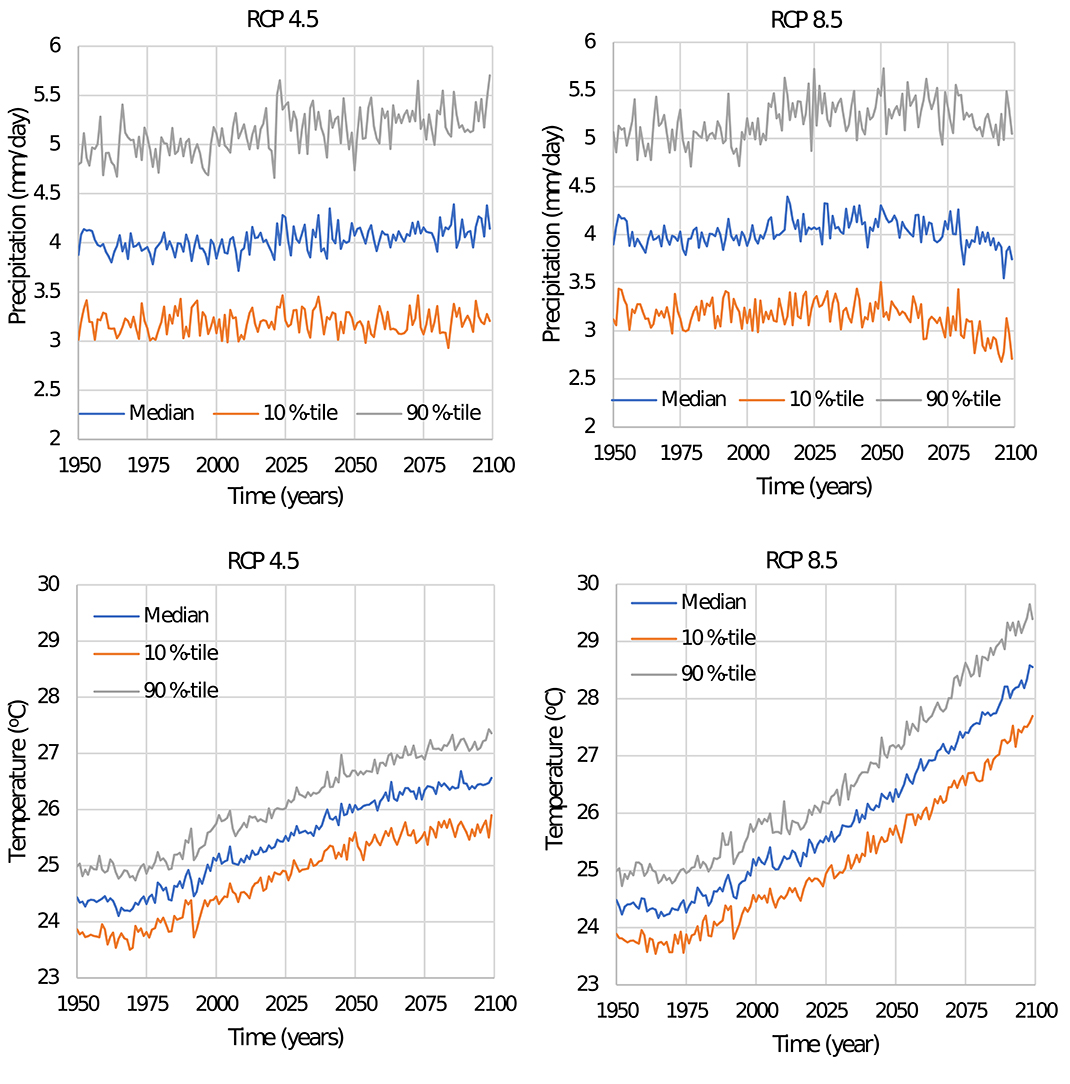
Figure 1. Projected 10 percentile, median, and 90 percentile values of precipitation and temperature for Miami.
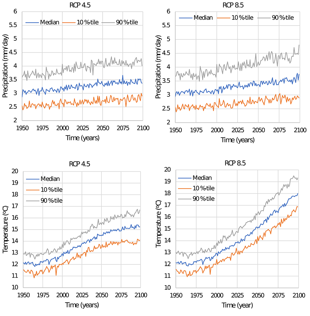
Figure 2. Projected 10 percentile, median, and 90 percentile values of precipitation and temperature for NYC.
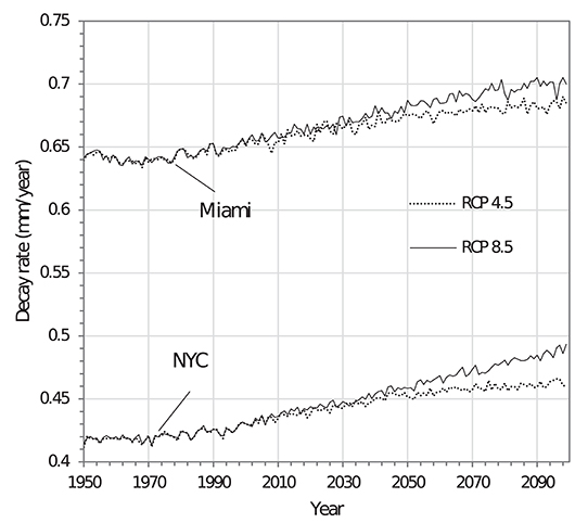
Figure 3. Impact of climate change on the decay rate (based on medians).
Hurricane Hazard Analysis
Hurricane Simulation
To model hurricane hazard, the hurricane simulation model developed by Xu and Brown (2008a) and also discussed in detail in Salman and Li (2016b) is adopted for use in this paper. The required parameters for the hurricane simulation in Florida are taken from Huang et al. (2001) and Xu and Brown (2008a). The parameters for NYC are found by fitting probability distributions to histograms of the parameters from Lin et al. (2010). The radial wind field model developed by Holland (1980) is used to calculate the gradient wind speed at locations of interest. The gradient wind speed is converted to a surface and then 3-s gust wind speed using factors of 0.8 and 1.287, respectively (Xu and Brown, 2008a; Vickery et al., 2009). The rise in central pressure (which results in weakening of intensity) of the hurricane after landfall is modeled using the approach developed by Vickery and Twisdale (1995). Wind speed decay after landfall due to friction and reduction in storm's moisture for Florida and New York are accounted for using the models developed by Kaplan and DeMaria (1995) and Kaplan and DeMaria (2001), respectively. Lastly, the radius to maximum wind is modeled using the equation from FEMA (2011). The simulation is carried out for 200,000 hurricane seasons. More details of the simulation model can be found in Salman and Li (2016b) and Salman and Li (2018).
Impact of Climate Change on Hurricane Hazard
Modeling the impact of climate change within the hurricane simulation model described above involve modifying the frequency and intensity parameters within the simulation. The impact of climate change on the frequency and intensity of future hurricanes has been a subject of much discussion. Some studies [e.g., Liu (2014)] have attempted to predict future hurricane activity based on the extrapolation of historical records. However, such an approach is constraint by the availability and quality of historical records and uncertain quantification of the natural variability in climate factors (IPCC, 2013). Hurricane formation and power dissipation depend on several climatic factors such as sea surface temperature (SST), North Atlantic Oscillation, Southern Oscillation, “El Nino” effect, vertical wind shear, atmospheric stability, and other factors (Ranson et al., 2014; Cui and Caracoglia, 2016). As such, variability in hurricane activity is a complex convolution of natural and anthropogenic factors. Studies that modeled the impact of climate change on hurricane activity using a physics-based approach mainly focused on the link between SST and hurricane formation (Mann and Emanuel, 2006; Mann et al., 2007; Elsner et al., 2008).
Since the relation between anthropogenic forcing and hurricane activities is not well-understood, there is no unified method of modeling climate change impact on hurricanes, and there is no consensus in the published literature on even the direction of the change. Table 1 summarized some of the reported changes in hurricane frequency and intensity in the literature. Note that the emission trajectory in A2 is similar to RCP 8.5, while RCP 4.5 is roughly between A1B–B1 (Inman, 2011). It can be seen from Table 1 that the range of reported change in the frequency and intensity of hurricanes due to climate change is large. Also, while some reported a potential increase in frequency, others reported a decrease. Most studies, however, reported an increase in intensity. The range of change in frequency and intensity under RCP 8.5 (and A2) in Table 1 are −25 to +55% and 0–25%, respectively. The corresponding values for frequency and intensity for RCP 4.5 (and A1B) are −62 to +58% and −10 to +12%, respectively.
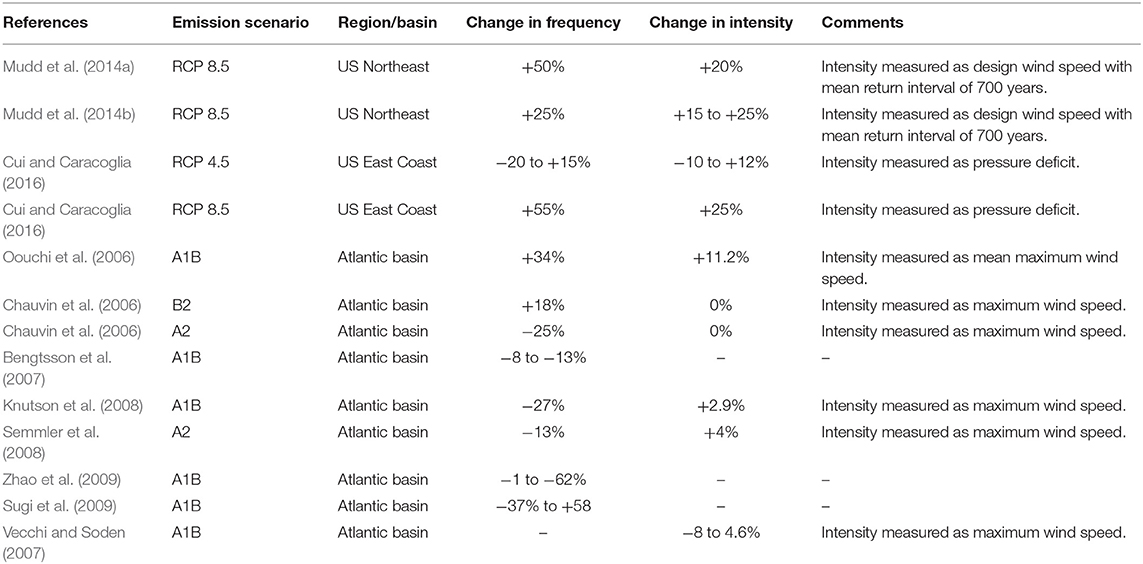
Table 1. Summary of research on the impact of climate change on hurricane frequency and intensity (only research that provides numerical values under specific emission scenarios are reported).
Based on the range of changes in frequency and intensity, the following scenarios are assumed at the end of the twenty-first century mostly following Mudd et al. (2014b) and Cui and Caracoglia (Cui and Caracoglia, 2016): (i) RCP 4.5 will result in no change in frequency and +12% change in intensity; and (ii) RCP 8.5 will result in +25% change in both frequency and intensity. While considerable inter- and intra-decadal variation in frequency and intensity of hurricanes exists, it is assumed here that the change in both frequency and intensity is linear from the start of the analysis, which is assumed to be 2010 in this case, to the end of the twenty-first century as suggested in Stewart et al. (2014) and Bastidas-Arteaga and Stewart (2015).
Optimal Replacement Model
Inspection of Poles
The National Electrical Safety Code (NESC) requires utility companies to regularly inspect and maintain the poles supporting power lines (NESC, 2017). The NESC also requires utilities to replace or reinforce poles whose strength falls below two-third of the initial strength due to decay. To comply with the NESC requirement, utilities typically carry out periodic inspections to identify poles that need maintenance. Considering the vast number of poles in distribution systems, it is neither practical nor economically feasible to frequently inspect all the poles in a system. Utility companies typically inspect a small percentage of the poles in their network every year. The number of years it takes to finish inspecting all the poles and start over is the length of the inspection cycle. For example, Florida Power & Light inspects 1/8 of its pole population every year as part of an 8-year pole inspection cycle plan. In a survey of 261 North American utilities, Mankowski et al. (2002) reported that the average inspection cycle for distribution poles is about 8 years. In the survey, utilities reported using a combination of inspection methods that include visual inspection, sounding with a hammer, boring with a drill, and the use of sonic devices. Similarly, Morrell (2008) studied the practices of US utilities and stated that most of the utilities inspect their poles on a 10-year cycle. In recent years, pole inspections are typically carried out using a mobile computing technology to record information such as pole class, species, ground-line circumference, year of manufacture, ID number, coordinate, span length, attachment heights, wire sizes, and data on condition assessment such as decay depth and chemical treatment.
Pole replacement can occur due to two reasons: (i) replacement due to damage by hurricane winds (corrective maintenance); and (ii) replacement due to excessive decay (preventive maintenance). In this research, the poles are assumed to be non-repairable components, i.e., failed or decayed poles are replaced with new ones. Because poles are constantly being replaced due to preventive and corrective maintenance, the age distribution of the poles in a network varies with time, and the poles can be divided into age groups.
Corrective Maintenance Model
The probability that a pole will be replaced due to hurricane winds in a given year is given by Equation (4).
where FR(v, t) is the time-dependent cumulative distribution function (CDF) of pole fragility and fv(v, t) is the time-dependent probability density function (PDF) of the annual maximum hurricane wind speed modeled by a Weibull distribution as discussed in section Hurricane hazard analysis. The expected number of poles that will be replaced (fail) annually due to hurricane winds for each age group is determined by multiplying the annual probability of failure with the total number of poles in the age group.
Preventive Replacement Model
Many maintenance models have been proposed in the literature and adopted in practice. These models can be generally grouped into two different approaches (Sánchez-Silva et al., 2016). The first group is the classic maintenance models that are based on only the observation of failure times or rates. In classic models, the actual deterioration mechanism is not explicitly considered. Rather, data on past failures of a component are used to determine its failure rate, which can then be used for maintenance optimization. Examples of classic models include models based on the renewal process (e.g., age and block replacement models). The second group is condition-based maintenance (CBM) models that account for the condition of the component or system at the time of the maintenance action. As such, these models require periodic or continuous inspection/condition monitoring. In these models, the rate of deterioration is typically modeled as a time-dependent stochastic process to account for uncertainties.
In this paper, two maintenance models are considered and compared.
Model 1: Replacement Based on Existing Inspection Cycle
In this model, poles whose strength falls below a certain threshold are identified and replaced during inspection. The inspection cycle is assumed to be 8 years long, based on the discussion in section Inspection of Poles. Note that in this case, deterioration is modeled using the empirical decay model presented earlier. As such, the inspection cycle here only indicates the points at which poles are replaced. The probability that a pole will be replaced due to maintenance is given by Equation (5), which is the probability that the strength of the pole at time t is less than the strength threshold for replacement.
where P is the probability of replacement; Rmin is the threshold strength for replacement; and fR(r, t) is the distribution function of pole strength, which is a function of time. The probability distribution of pole strength is determined based on the decay model. The minimum strength at which poles will be replaced due to maintenance (Rmin) is based on the threshold specified by NESC (2017), which is two-third of the original design strength of the pole. The expected number of same-age poles to be replaced follows a binomial distribution and is given by the product of the number of poles in an age group and the probability of replacement, P, in Equation (5).
Model 2: Replacement Based on Optimization
In the second model, a CBM optimization approach is considered. In a CBM approach, the deterioration process is typically modeled as a time-dependent stochastic process. Therefore, this section will first focus on stochastic modeling of decay processes by accounting for the empirical decay model and climate change provided in section Wood decay model. Stochastic processes such as the gamma process can be employed in CBM to model the deterioration or decay process. For monotonic and gradual deterioration, the gamma process is deemed to be the most appropriate, and it has been used successfully in maintenance optimization because it is well-suited for modeling the temporal variability of deterioration processes (Van Noortwijk, 2009). Therefore, the gamma process is used in this case to model the decay of the wood poles. Let X(t) be a random variable denoting the deterioration of the poles at time t. The deterioration is then a stochastic gamma process {X(t), t≥0}, with the following properties (Rausand and Høyland, 2004):
i. X(0) = 0.
ii. {X(t), t≥0} has independent increments.
iii. For all 0 ≤ s < t, the random variable X(t)−X(s) has a gamma distribution with parameters (α(t−s), β) and probability density function (PDF)
where Γ(·) denotes the gamma function.
If X(t) is a gamma process with shape function α(t) and an inverse scale parameter β, then the expected deterioration and variance are given by (Frangopol et al., 2004):
In modeling deterioration with a gamma process, the expected deterioration at time t is often proportional to a power law (Frangopol et al., 2004; Van Noortwijk, 2009):
In this case, the deterioration is the decay depth as a function of time. As an example, the decay depth for a pole is plotted in Figure 4 for the case of no climate change and RCP 8.5 (mean inputs) for Miami. For the case of no climate change, the average decay rate between 1950 and 2010 is used, i.e., the decay rate is constant, and decay depth is linear with time. For the climate change case, the decay rate varies with time depending on the variation in temperature and precipitation. However, because the annual variation in the decay rate is small (see Figure 3), the decay depth (cumulative decay) is also approximately linear. As such, for both cases, it can be concluded that b in Equation (8) is equal to 1 since the expected deterioration is approximately a linear function of time. As such, the cumulative decay has a stationary gamma-distributed independent increments. Similar trends are observed for NYC and all climate change scenarios.
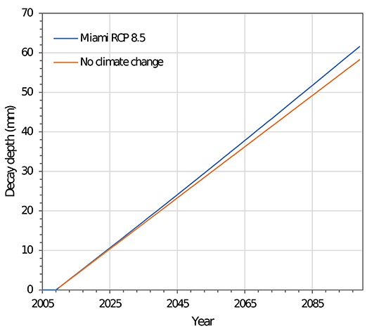
Figure 4. Variation of decay depth with time for Miami.
Since the deterioration is a stationary gamma process defined by a linear shape function, the corresponding probability density function of X(t) is then given by:
To develop the optimization model, the following assumptions are made:
1. The deterioration (decay depth) is a random process that is non-decreasing as a function of time measured on a continuous scale and modeled by a gamma process.
2. The poles are inspected at regular intervals and, therefore, replacements are carried out at regular intervals.
3. When the estimated decay is greater than the NESC decay threshold, the pole is preventively replaced at the first inspection when the threshold is passed.
4. Decayed poles are replaced with new ones of the same class. Hence, after replacement, the poles are as good as new.
5. The inspection is perfect, i.e., any decay present will be detected and measured with a negligible error.
Let ΔXi be the decay within inspection interval i, for i = 1, 2, …. Since the decay is a gamma process, ΔX1, ΔX2, …, will be independent and gamma-distributed with distribution function F(x) (Rausand and Høyland, 2004). If the poles are inspected after regular intervals of length τ; the cost of inspection, preventive replacement, and additional cost of corrective replacements are Ci, Cp, and Cc; and the mean number of inspections before preventive replacement is np, then following Rausand and Høyland (2004), the average cost per replacement cycle is:
Since crossing of the replacement decay threshold is only detected in the first inspection after it has been exceeded, the crossing will be detected in inspection (np+1). The expected total cost per unit time is then given by Equation (11).
Equation (11) can be used to determine the optimal inspection interval, τ, that minimizes the expected total cost per unit time, C(τ).
To determine Pr(failure), two deterioration or condition levels are set: the “critical” level, yp, and the “failure” level, yc. Once the condition of the pole reaches the “critical” level, it is preventively replaced to avoid failure. The “critical” level, in this case, is based on the NESC requirement mentioned earlier, which is when the strength will fall below 2/3 of the initial strength. The “failure” level, yc, is higher than yp, and is the deterioration level that can jeopardize the functionality of the pole. The value of yc can be set based on experience or field observations. Note that a failure, (X(t)>yc), is not detected immediately until the next inspection. The expected total cost per unit time is then given by Equation (12).
Based on previous discussion, F(yc−yp) in Equation (12) has a gamma distribution with a PDF given by Equation (6) and parameters ατ and β (with τ = t−s). The term [(np+1)·τ] in Equation (12) is the expected cycle length given by Equation (13) (Rausand and Høyland, 2004).
where μτ is the mean decay in an inspection interval and μ is the slope of the plot of the cumulative decay depth with time.
Illustrative Example
Pole Network Description
To demonstrate the proposed framework, a network of 200,000 southern pine poles in Miami and NYC is considered. Southern pine is selected because it is the dominant specie used in the U.S. to support distribution lines (Wolfe and Moody, 1997). The durability class is assumed to be class 1 based on the service life of the poles used, as discussed below. The poles are also assumed to be size class 4, according to ANSI-O5.1 (2002) classification. They are also assumed to be typical distribution poles supporting three Aluminum Conductor Steel Reinforced (ACSR) conductor wires with diameters of 18.3 mm and one all-aluminum conductor (AAC) neutral wire with a diameter of 11.8 mm. The span between poles is taken as 46 m (Short, 2005).
As poles in a network are constantly being replaced due to failure or excessive decay, the age of the poles in a network varies considerably. A study of the wood poles in Florida after Hurricane Wilma shows that the age of poles varies from 1 to 49 years (KEMA, 2006). The pole age distribution shown in Figure 5 is used in this research and is based on data compiled by KEMA (2006) for a utility company in Florida in 2005. The spike for poles that are 13 years old is due to the high number of failed poles caused by Hurricane Andrew. A survey of ~100,000 poles in Canada by Datla and Pandey (2006) also shows the age of most of the poles varies between 1 and 60 years with near-uniform distribution.
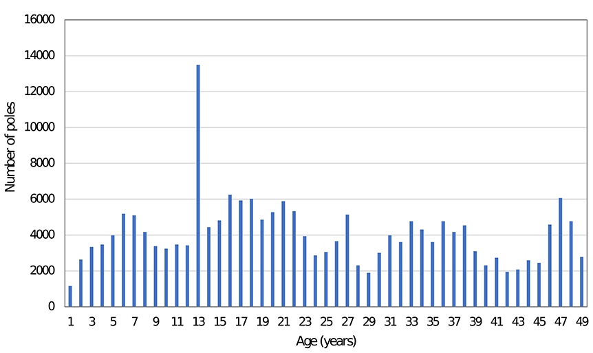
Figure 5. Age distribution of poles.
Corrective Maintenance Only Results
In this section, it is assumed that only corrective maintenance is carried out, i.e., poles are only replaced when they fail due to hurricane winds. Time-dependent decrease in strength due to decay is considered in the hurricane winds-induced failures. However, preventive replacement is not carried out. This scenario is considered because, according to a survey of utility companies in the U.S. by Mankowski et al. (2002), some utilities reported having an inspection and preventive maintenance program for transmission but not distribution poles.
The period considered is 2010–2099. The analysis starts in 2010 with the pole age distribution shown in Figure 5. The annual probability of failure in 2010 for each age group is then calculated using Equation (4). The mean number of failed poles in an age group is then the annual probability of failure multiplied by the number of poles in that age group. Failed poles are replaced with new poles of the same class. In the following year (2011), the decay rate is sampled from the distribution of climate parameters in that year and the strength of the poles is then updated. The annual probabilities of failure and the mean number of failed poles for each age group in 2011 is then calculated. This procedure is repeated until 2099. To determine the annual probabilities of failure, the time-dependent fragility of the poles is required. Details and data for the fragility analysis are given in Appendix A.
The average annual failure rates of poles in Miami in the case of no climate change is shown in Figure 6A. The average annual replacement rate is about 3.8% between 2010 and 2030, after which it drops to about 3.4% as older poles are replaced with new ones after failure. These percentages are, however, annual averages. Historically, the percentage of failed poles after a hurricane can vary significantly. For example, after Hurricane Wilma, Florida Power & Light had to replace 1.5% of poles exposed to hurricane winds. After Hurricane Andrew, the percentage of replaced poles was about 10.1% (KEMA, 2006).
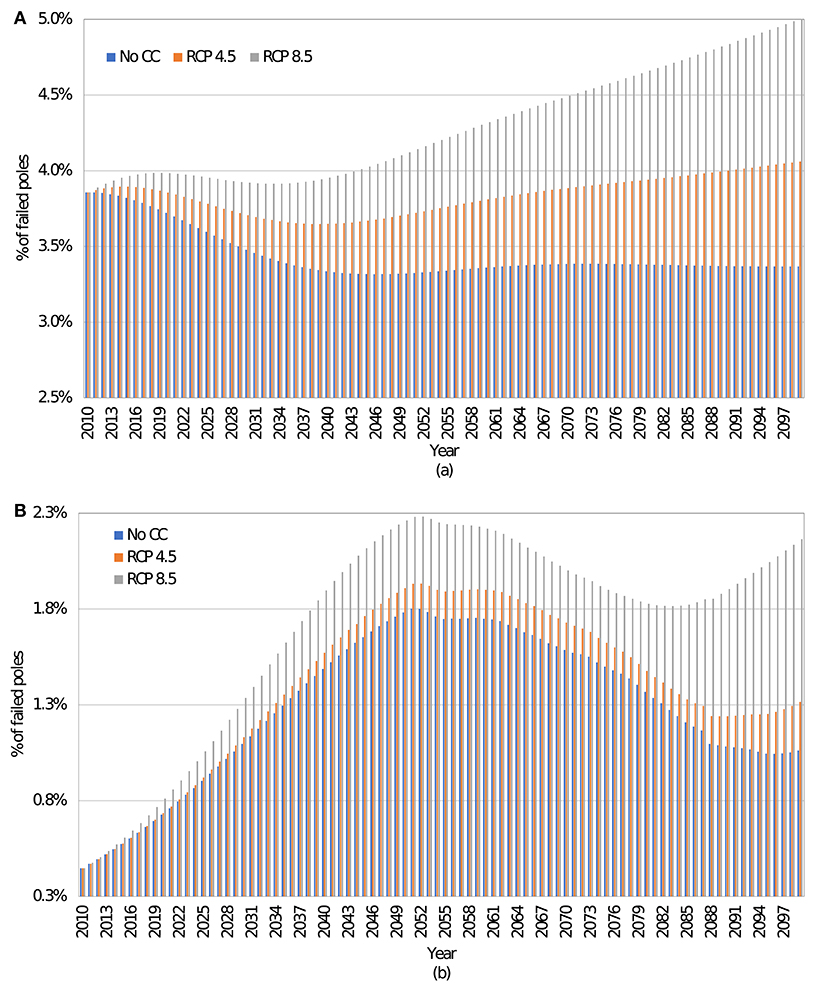
Figure 6. Percentage of failed poles in (2010–2099) (A) Miami (B) NYC.
With climate change, the average annual replacement rate in Miami between 2010 and 2030 is 3.8 and 3.9% for RCP 4.5 and RCP 8.5, respectively, as shown in Figure 6A. It then changed to 3.7 and 4.2% between 2030 and 2070, respectively. After 2070, the average increased to 4 and 4.8%, respectively. For NYC, the average annual replacement rates for the periods 2010–2030, 2030–2070, and 2070–2099 with no climate change are 0.7, 1.6, and 1.2%, respectively, as seen in Figure 6B. For RCP 4.5, the replacement rates are 0.7, 1.7, and 1.4%, respectively, for the same periods. For RCP 8.5, the replacement rates are 0.8, 2, and 1.9%, respectively, for the same period. The increase in replacement rates between 2030 and 2070 is due to the aging of existing poles while the eventual decrease between 2070 and 2099 is due to the replacement of aged poles with new ones.
Comparing the patterns of the number of failed poles with and without climate change in Miami, it can be seen that with no climate change, the pattern starts with a decrease in the number of failed poles from 2010. This is because failed poles are replaced with new ones, and the annual probability of failure of poles of specific age does not increase with time. The annual number of failed poles then increases slightly after 2046 as the poles age. However, with climate change, the number of failed poles increases slightly after 2010 before eventually decreasing. This is because even though failed poles are replaced with new ones, the annual probability of failure is increasing. As such, it takes a while for enough new poles to be installed to lead to an overall decrease in the number of failed poles despite an increase in the annual probability of failure. However, with climate change, the annual number of failed poles eventually starts to increase significantly due to aging and an increase in the annual failure probability for poles of a specific age. In NYC, the pattern remained largely the same with and without climate change due to the low hurricane risk.
Note that with climate change, the total decay depth for two poles of the same age will be different depending on the year of installation. For example, a pole that is 10 years old in 2070 (installed in 2060) will have a higher total decay depth compared to a pole that is 10 years old in 2040 (installed in 2030). Hence, the annual probability of failure will also be different. For example, the annual probability of failure of a 10-year-old pole in Miami under RCP 8.5 increased from 1.85% in 2010 to 2.67% and 3.73% in 2050 and 2099, respectively, due to climate change.
Figure 7 shows the total number of failed poles between 2010 and 2099 with and without climate change for Miami and NYC. As expected, climate change increased the total number of failed poles in Miami by about 9 and 22% for RCP 4.5 and RCP 8.5, respectively. In NYC, the corresponding increase is about 8 and 35% for RCP 4.5 and RCP 8.5, respectively. The relatively higher increase in NYC for RCP 8.5 compared to Miami can be attributed to an increase in precipitation and, consequently, a higher increase in decay rate, as discussed in section Impact of Climate Change on Decay Rate.
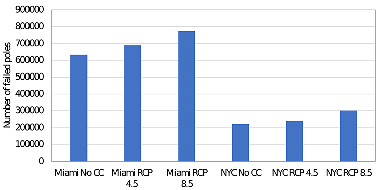
Figure 7. Comparison of the total number of failed (replaced) poles (2010–2099).
Preventive and Corrective Replacement Results
In this section, results combining corrective replacement (due to hurricanes, considering decay) and preventive replacement (due to decay only) are presented.
Model 1: Replacement Based on Existing Inspection Cycle
The 200,000 poles are assumed to be a sub-set of the total poles in a large network. All the poles in the sub-set are inspected every 8 years as discussed in section Preventive replacement model, with the first inspection carried out in 2010. Poles whose strength falls below two-third of the initial strength are identified and replaced with new ones during the inspection, as discussed earlier. Poles that fail due to hurricane winds are also replaced with new ones. The total number of replaced poles in any year is the summation of the two (corrective and preventive replacements).
Figure 8A shows the average annual percentage of poles replaced, considering both corrective and preventive replacement in Miami. The spikes in the figure are preventive replacements every 8 years, while the others are yearly corrective replacement. It can be seen that over 40% of the poles in the network will be replaced in 2010 due to preventive maintenance. This is because, based on the decay model adapted here, the time until a pole reaches two-third of its initial strength (time until replacement) is about 30 years. However, based on the age distribution of the poles in the network shown in Figure 5, about 35% of the poles are over 30 years old. The percentage of replaced poles due to preventive maintenance eventually decreased as the average pole age decreased due to the initial high replacement rate.
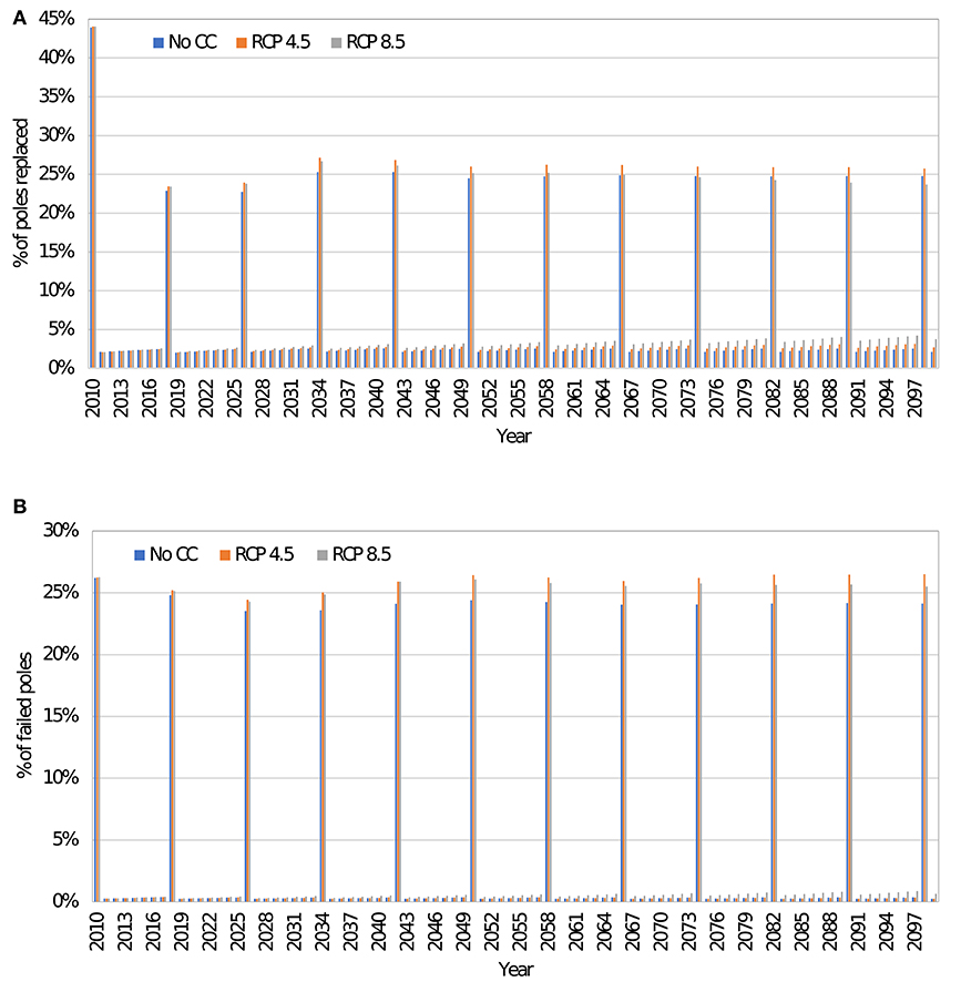
Figure 8. Percentage of poles replaced (8-year inspection cycle) (A) Miami (B) NYC.
Figure 8B shows the percentage of replaced poles in NYC. The average percentage of poles replaced due to preventive maintenance in 2010 is about 26%. It is lower than in Miami because of the lower decay rate in NYC. It should be emphasized that the decay model used in this study is for the purpose of demonstrating the proposed framework. Utility companies can develop their decay models based on wood and climate data collected over a period.
Figure 9 shows a comparison of corrective replacement only and corrective + preventive replacement in Miami with no climate change. It is seen that preventive replacement decreases the annual corrective replacement rate due to hurricanes as expected. However, the total number of replaced poles between 2010 and 2099 for the case of corrective replacement only is still lower than the total for the case of preventive + corrective replacement due to the high preventive replacement rate. The cases with climate change show similar trends.
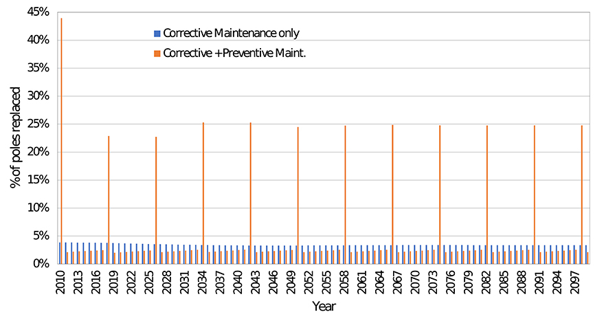
Figure 9. Comparison of the number of replaced poles for corrective only and corrective + preventive replacement for Miami with no CC (8-year inspection cycle).
Model 2: Replacement Based on Optimization
To determine the optimal inspection cycle for network, the cost parameters in Table 2 are used. Only direct costs are included in this table. In addition to the cost parameters, the failure level, yc, needs to be defined. Recall that the critical level, yp, is the deterioration level that causes the strength of the pole to fall below 67% of the initial strength as specified by NESC. The 67% level is the decay level at which the pole strength is expected to be about the same as the design load. Hence, deterioration below the 67% level will likely lead to failure of the pole under design loads. Since yc is expected to be less than yp, for the sake of comparison, yc is henceforth assumed to be the deterioration level that will cause the strength of the pole to be <60% of the initial strength. Based on this assumption, the optimal inspection cycles for Miami with no climate, RCP 4.5, and RCP 8.5 are 9, 8, and 8 years, respectively. The corresponding optimal cycles for NYC are 14, 13, and 13, respectively. The higher values in NYC are due to lower decay rates, as seen in Figure 3. It is seen that climate change has only a small impact on the optimal inspection cycles, decreasing the values by one year in both locations. Note that if yc is taken as the deterioration corresponding to 55% of initial strength, the optimal inspection cycles for Miami increase to 17, 16, and 16 years for no climate change, RCP 4.5, and RCP 8.5, respectively. The corresponding values for NYC will be 27, 26, and 25 years, respectively. The increase in the optimal solutions is due to an increase in decay tolerance. The average annual percentage of poles replaced based on the optimal solutions will have similar trends seen in Figures 8, 9.
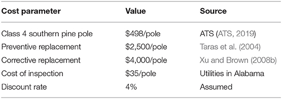
Table 2. Cost analysis parameters.
Comparison of Cost Results
The present value of the total cost of pole replacement between 2010 and 2099 with and without climate change for the two locations is evaluated. The results are shown in Figure 10 for the cases of only corrective replacement and combined corrective + preventive replacement (8-year cycle and the optimal cycles). Climate change increases the total cost in both locations. Based on the 8-year inspection cycle, RCP 4.5 and RCP 8.5 increased the total replacement cost by 4 and 8%, respectively, in Miami. The corresponding increase is 3 and 6%, respectively, in NYC. Based on the optimal inspection cycle, RCP 4.5 and RCP 8.5 increased the total replacement cost by 7 and 10%, respectively, in Miami. The corresponding increase is 2 and 6%, respectively, in NYC.
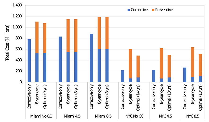
Figure 10. Comparison of total replacement costs from 2010 to 2099.
Including preventive maintenance increased the total cost in all cases. Preventive replacement increased the total discounted cost by 35–41 and 94–175% in Miami and NYC, respectively. This is because of the high number of poles that need to be replaced, as discussed previously. It is also because the corrective replacement cost is not significantly higher than the preventive replacement cost, as seen in Table 2. Note that considering down time of the system and unplanned power outage as well as possible damage and hazard to the public caused by the failed pole, the actual cost of a corrective replacement would be higher than the assumed value in Table 2. If the corrective replacement cost is significantly larger than the preventive cost, then implementing the preventive maintenance will be cost-effective. The corrective replacement cost will be larger if additional expenditures (indirect costs) related for example with the disruption of the service are considered in the cost assessment. However, these indirect costs were not considered because of the lack of reliable data to assess it. The higher increase in the total cost due to the preventive maintenance in NYC is due to the lower hurricane risk and decay rate. As such, preventive maintenance is more beneficial in Miami compared to NYC. Preventive replacement reduces the cost of corrective maintenance for all cases. It decreased the corrective maintenance cost by 32–34% and 57–70% in Miami and NYC, respectively. This is because of the reduced failure risk due to having newer poles in the network as a result of the preventive maintenance strategy.
In general, an increase in the length of the inspection cycle decreases the preventive maintenance cost while increasing the corrective maintenance cost because more decayed poles being left in service. It should be noted that the comparison here is only based on cost. Other considerations, especially component and system reliability, are also important. For example, the NESC requirement to replace poles whose strength falls below two-third of the initial strength is based on reliability consideration.
Conclusions
This paper presents a framework to optimize the maintenance of a network of wood utility poles subjected to decay and hurricane hazard. The framework can be used by utility companies to determine the optimal inspection cycle for a network of poles. Two coastal locations are considered as case studies to investigate the variation of the results for different geographical conditions: Miami, Florida, and New York City, New York. The period from 2010 to 2099 is considered for the study. The impact of climate change on decay, hurricane hazard, and pole failure and replacement rate was also investigated. The correlation between strong winds during storms or hurricanes, and intense rainfall (that could modify the decay rate) is not considered in this work. Considering this correlation requires global circulation models able to simulate storms or hurricanes. Further studies will investigate the effects of this correlation when these models become available. The results of the case studies show that the proposed framework can be used to determine the optimal inspection/replacement cycle to minimize the total maintenance cost.
Based on a comparison between current typical utility maintenance practice and the optimization results, it can be concluded that the current maintenance practice by utility companies may not be the optimal approach based on cost. The optimal inspection/replacement cycle depends on location, which dictates the decay rate and hurricane hazard level. The results also show that climate change has little impact on the optimal inspection cycle. It can, however, increase the total maintenance cost over time due to the increased likelihood of failure of the poles caused by a higher decay rate and hurricane winds. Based on the current typical 8-year inspection cycle used by some utilities, climate change can increase the total maintenance cost by up to 8% in Miami and 6% in NYC, depending on the emission scenario considered.
Optimal inspection intervals where formulated for each location and climate change scenario. However, the cost-effectiveness of the inspection solutions could be improved by considering flexible inspection times to take into account, in a comprehensive way, the deep uncertainties associated to the climate-related complexity. For example, the highest level of deep uncertainty “True ambiguity” (Helmrich and Chester, 2020) considers the more realistic scenario where the future cannot be predicted. To face this scenario, inspection times should be defined and updated taking into account the feedback from a given number of years of operation under a real climate as well as new climate change predictions at the moment of the assessment/updating. Further work will be addressed to the formulation of optimal and flexible maintenance planning considering this level of deep uncertainty.
The results of the case studies show that implementing a preventive maintenance strategy decreases the number of poles that fail due to hurricane winds. However, it increases the total maintenance cost. While this may indicate that it is desirable to only carry out corrective maintenance, the results are true for the specific cost values used in the case studies that neglect indirect costs. Also, only the direct cost of damage is considered in this study. Indirect costs such as revenue loss by utility companies and losses to customers due to power outages are not considered. Other factors, such as reliability and customer satisfaction, can also affect the decision to adopt a preventive maintenance plan.
Data Availability Statement
The datasets generated for this study can be obtained from the corresponding author upon request.
Author Contributions
AS, EB-A, and YL contributed to the conception and design of the study. AS and BS performed the computations. AS and E-BA wrote the manuscript. E-BA and YL revised the work critically for important intellectual content. All authors contributed to manuscript revision, read and approved the submitted version.
Conflict of Interest
The authors declare that the research was conducted in the absence of any commercial or financial relationships that could be construed as a potential conflict of interest.
Acknowledgments
We acknowledge the modeling groups, the Program for Climate Model Diagnosis and Intercomparison (PCMDI) and the WCRP's Working Group on Coupled Modeling (WGCM) for their roles in making available the WCRP CMIP3 and CMIP5 multi-model dataset. Support of this dataset is provided by the Office of Science, U.S. Department of Energy.
References
ANSI-O5.1 (2002). Wood Poles Specifications and Dimensions. Washington, DC: American National Standards Institute.
ASCE (2015). Adapting Infrastructure and Civil Engineering Practice to a Changing Climate (R. Olsen Ed.). Reston, VA: American Society of Civil Engineers - Committee on Adaptation to a Changing Climate.
ASCE-111 (2006). Reliability-Based Design of Utility Pole Structures. Reston, VA: American Sociaety of Civil Engineers.
ATS (2019). Products and Pricing. Retrieved from: http://www.americantimberandsteel.com/poles-pilings-utility-poles-unframed-cca.html (accessed October 15, 2019).
AWPA (2014). U1-14 Use Category System: User Specification for Treated Wood. Birmingham, AL: American Wood Protection Association.
Bastidas-Arteaga, E., Aoues, Y., and Chateauneuf, A. (2015). Optimal Design of New Deteriorating Timber Components Under Climate Variations. Paper presented at the 12th International Conference on Applications of Statistics and Probability in Civil Engineering (ICASP12).
Bastidas-Arteaga, E., and Stewart, M. G. (2015). Damage risks and economic assessment of climate adaptation strategies for design of new concrete structures subject to chloride-induced corrosion. Structural Safety 52, 40–53. doi: 10.1016/j.strusafe.2014.10.005
Bender, M. A., Knutson, T. R., Tuleya, R. E., Sirutis, J. J., Vecchi, G. A., Garner, S. T., et al. (2010). Modeled impact of anthropogenic warming on the frequency of intense Atlantic hurricanes. Science 327, 454–458. doi: 10.1126/science.1180568
Bengtsson, L., Hodges, K. I., Esch, M., Keenlyside, N., Kornblueh, L., LUO, J. J., et al. (2007). How may tropical cyclones change in a warmer climate? Tellus 59, 539–561. doi: 10.1111/j.1600-0870.2007.00251.x
Bjarnadottir, S., Li, Y., Reynisson, O., and Stewart, M. G. (2018). Reliability-based assessment of climatic adaptation for the increased resiliency of power distribution systems subjected to hurricanes. Sustain. Resilient Infrastruct. 3, 36–48. doi: 10.1080/23789689.2017.1345255
Bjarnadottir, S., Li, Y., and Stewart, M. (2013). Hurricane risk assessment of power distribution poles considering impacts of a changing climate. J. Infrastruct. Syst. 19, 12–24. doi: 10.1061/(ASCE)IS.1943-555X.0000108
Brischke, C., and Rapp, A. O. (2008). Influence of wood moisture content and wood temperature on fungal decay in the field: observations in different micro-climates. Wood Sci. Tech. 42:663. doi: 10.1007/s00226-008-0190-9
Chauvin, F., Royer, J.-F., and Déqué, M. (2006). Response of hurricane-type vortices to global warming as simulated by ARPEGE-Climat at high resolution. Clim. Dyn. 27, 377–399. doi: 10.1007/s00382-006-0135-7
Cui, W., and Caracoglia, L. (2016). Exploring hurricane wind speed along US Atlantic coast in warming climate and effects on predictions of structural damage and intervention costs. Eng. Struct. 122, 209–225. doi: 10.1016/j.engstruct.2016.05.003
Datla, S., and Pandey, M. (2006). Estimation of life expectancy of wood poles in electrical distribution networks. Structural Safety 28, 304–319. doi: 10.1016/j.strusafe.2005.08.006
De Larrard, T., Bastidas-Arteaga, E., Duprat, F., and Schoefs, F. (2014). Effects of climate variations and global warming on the durability of RC structures subjected to carbonation. Civ. Eng. Environ. Syst. 31, 153–164. doi: 10.1080/10286608.2014.913033
Edwards, T. (2013). “Hydrometeorological hazards under future climate change,” in Risk and Uncertainty Assessment for Natural Hazards, eds J. Rougier, S. Sparks, and L. Hill, 151:151–189. doi: 10.1017/CBO9781139047562.007
Ellingwood, B. R., and Tekie, P. B. (1999). Wind load statistics for probability-based structural design. J. Struct. Eng. 125, 453–463. doi: 10.1061/(ASCE)0733-9445(1999)125:4(453)
Elsner, J. B., Kossin, J. P., and Jagger, T. H. (2008). The increasing intensity of the strongest tropical cyclones. Nature, 455, 92–95. doi: 10.1038/nature07234
FEMA (2011). Multi-Hazard Loss Estimation Methodology, Hurricane Model: Hazus-MH 2.1 Technical Manual. Washington, DC: FEMA.
Frangopol, D. M., Kallen, M. J., and Van Noortwijk, J. M. (2004). Probabilistic models for life-cycle performance of deteriorating structures: review and future directions. Progress in Struct. Eng. Mater. 6, 197–212. doi: 10.1002/pse.180
Gere, J. M., and Carter, W. O. (1962). Critical buckling loads for tapered columns. ASCE 88(ST1, Part 1), 1–11.
Gustavsen, B., and Rolfseng, L. (2000). Simulation of wood pole replacement rate and its application to life cycle economy studies. IEEE Transact. Power Delivery 15, 300–306. doi: 10.1109/61.847266
Gustavsen, B., Rolfseng, L., Andresen, O., Christensen, H., Falch, B., Jankila, K. A., et al. (2002). Simulation of wood-pole replacement rate: application to distribution overhead lines. IEEE Transact. Power Delivery 17, 1050–1056. doi: 10.1109/TPWRD.2002.800879
Helmrich, A. M., and Chester, M. V. (2020). Reconciling complexity and deep uncertainty in infrastructure design for climate adaptation. Sustain. Resilient Infrastructure. doi: 10.1080/23789689.2019.1708179. [Epub ahead of print].
Holland, G. J. (1980). An analytic model of the wind and pressure profiles in hurricanes. Monthly Weather Review 108, 1212–1218. doi: 10.1175/1520-0493(1980)108<1212:AAMOTW>2.0.CO;2
Huang, Z., Rosowsky, D., and Sparks, P. (2001). Hurricane simulation techniques for the evaluation of wind-speeds and expected insurance losses. J. Wind Eng. Industr. Aerodyn. 89, 605–617. doi: 10.1016/S0167-6105(01)00061-7
IPCC (2013). “Climate Change 2013: The Physical Science Basis,” in Contribution of Working Group I to the Fifth Assessment Report of the Intergovernmental Panel on Climate Change, eds T. F. Stocker, D. Qin, G.-K. Plattner, M. Tignor, S.K. Allen, J. Boschung, A. Nauels, Y. Xia, V. Bex and P.M. Midgley (Cambridge; New York, NY: Cambridge University Press), 1552.
Isaksson, T., Brischke, C., and Thelandersson, S. (2013). Development of decay performance models for outdoor timber structures. Mater. Struct. 46, 1209–1225. doi: 10.1617/s11527-012-9965-4
Kaplan, J., and DeMaria, M. (1995). A simple empirical model for predicting the decay of tropical cyclone winds after landfall. J. Appl. Meteorol. 34, 2499–2512. doi: 10.1175/1520-0450(1995)034<2499:ASEMFP<2.0.CO;2
Kaplan, J., and DeMaria, M. (2001). On the decay of tropical cyclone winds after landfall in the New England area. J. Appl. Meteorol. 40, 280–286. doi: 10.1175/1520-0450(2001)040<0280:OTDOTC>2.0.CO;2
KEMA (2006). Post Hurricane Wilma Engineering Analysis. Retrieved from: https://www.coursehero.com/file/34562321/FPL-Pre-Workshop-Responses-Wilma-1doc/ (accessed October 15, 2019).
Knutson, T. R., Sirutis, J. J., Garner, S. T., Vecchi, G. A., and Held, I. M. (2008). Simulated reduction in Atlantic hurricane frequency under twenty-first-century warming conditions. Nat. Geosci. 1:359. doi: 10.1038/ngeo202
Leicester, R. H., Wang, C.-H., Nguyen, M. N., and MacKenzie, C. E. (2009). Design of exposed timber structures. Austral. J. Struct. Eng. 9, 217–224. doi: 10.1080/13287982.2009.11465024
Lin, N., Emanuel, K., Smith, J., and Vanmarcke, E. (2010). Risk assessment of hurricane storm surge for New York City. J. Geophys. Res. (Clemson, SC:Clemson, SC), 115:D18121. doi: 10.1029/2009JD013630Clemson, SC:
Liu, F. (2014). Projections of Future US Design Wind Speeds Due to Climate Change for Estimating Hurricane Losses. Clemson University.
Mankowski, M., Hansen, E., and Morrell, J. (2002). Wood pole purchasing, inspection, and maintenance: a survey of utility practices. Forest Products J. 52:43. Available online at: https://search.proquest.com/docview/214640466/fulltext/4C855739DA104949PQ/1?accountid=14476
Mann, M. E., and Emanuel, K. A. (2006). Atlantic hurricane trends linked to climate change. Transact. Am. Geophys. Union 87, 233–244. doi: 10.1029/2006EO240001
Mann, M. E., Sabbatelli, T. A., and Neu, U. (2007). Evidence for a modest undercount bias in early historical Atlantic tropical cyclone counts. Geophys. Rese. Lett. 34:L22707. doi: 10.1029/2007GL031781
Maurer, E. P., Brekke, L., Pruitt, T., and Duffy, P. P. (2007). Fine-resolution climate projections enhance regional climate change impact studies. Eos Transact. Am. Geophys. Union 88:504. doi: 10.1029/2007EO470006
Morrell, J. J. (2008). Estimated service life of wood poles. Technical Bulletin, North American Wood Pole Council. Available online at: http://www.woodpoles.org/documents/TechBulletin_EstimatedServiceLifeofWoodPole_12-08.pdf (accessed April 5, 2013).
Moss, R. H., Edmonds, J. A., Hibbard, K. A., Manning, M. R., Rose, S. K., Van Vuuren, D. P., et al. (2010). The next generation of scenarios for climate change research and assessment. Nature 463, 747–756. doi: 10.1038/nature08823
Mudd, L., Wang, Y., Letchford, C., and Rosowsky, D. (2014a). Assessing climate change impact on the US East Coast hurricane hazard: temperature, frequency, and track. Nat. Hazards Rev. 15:04014001. doi: 10.1061/(ASCE)NH.1527-6996.0000128
Mudd, L., Wang, Y., Letchford, C., and Rosowsky, D. (2014b). Hurricane wind hazard assessment for a rapidly warming climate scenario. J. Wind Eng. Industr. Aerodyn. 133, 242–249. doi: 10.1016/j.jweia.2014.07.005
Nguyen, M., Foliente, G., and Wang, X. M. (2004). State-of-the-practice and challenges in non-destructive evaluation of utility poles in service. Key Eng. Mater. (Trans Tech Publications Ltd), 1521–28. doi: 10.4028/www.scientific.net/KEM.270-273.1521
Oouchi, K., Yoshimura, J., Yoshimura, H., Mizuta, R., Kusunoki, S., and Noda, A. (2006). Tropical cyclone climatology in a global-warming climate as simulated in a 20 km-mesh global atmospheric model: frequency and wind intensity analyses. J. Meteorol. Soc. Ser. II 84, 259–276. doi: 10.2151/jmsj.84.259
Peng, L., and Stewart, M. G. (2014). Spatial time-dependent reliability analysis of corrosion damage to RC structures with climate change. Magaz. Concrete Res. 66, 1154–1169. doi: 10.1680/macr.14.00098
Peters, G. P., Andrew, R. M., Boden, T., Canadell, J. G., Ciais, P., Le Quere, C., et al. (2013). The challenge to keep global warming below 2 [deg]C. Nat. Clim. Change, 3, 4–6. doi: 10.1038/nclimate1783
Quanta-Technology (2009). Cost-Benefit Analysis of the Deployment of Utility Infrastructure Upgrades and Storm Hardening Programs. Raleigh: Quanta Technology.
Ranson, M., Kousky, C., Ruth, M., Jantarasami, L., Crimmins, A., and Tarquinio, L. (2014). Tropical and extratropical cyclone damages under climate change. Climatic Change 127, 227–241. doi: 10.1007/s10584-014-1255-4
Rausand, M., and Høyland, A. (2004). System Reliability Theory: Models, Statistical Methods, and Applications (Vol. 396). Hoboken, NJ: John Wiley and Sons.
Ryan, P. C., and Stewart, M. G. (2017). Cost-benefit analysis of climate change adaptation for power pole networks. Climatic Change 143, 519–533. doi: 10.1007/s10584-017-2000-6
Salman, A. M., and Li, Y. (2016a). Age-dependent fragility and life-cycle cost analysis of wood and steel power distribution poles subjected to hurricanes. Struct. Infrastruct. Eng. 12, 890–903. doi: 10.1080/15732479.2015.1053949
Salman, A. M., and Li, Y. (2016b). Assessing climate change impact on system reliability of power distribution systems subjected to hurricanes. J. Infrastruct. Syst, 23. doi: 10.1061/(ASCE)IS.1943-555X.0000316
Salman, A. M., and Li, Y. (2018). A framework to investigate the effectiveness of interconnection of power distribution systems subjected to hurricanes. Struct. Infrastruct. Eng. 14, 203–217. doi: 10.1080/15732479.2017.1345954
Salman, A. M., Li, Y., and Bastidas-Arteaga, E. (2017). Maintenance optimization for power distribution systems subjected to hurricane hazard, timber decay and climate change. Reliabil. Eng. Syst. Safety. 142, 111–122. doi: 10.1016/j.ress.2017.03.002
Sánchez-Silva, M., Frangopol, D. M., Padgett, J., and Soliman, M. (2016). Maintenance and operation of infrastructure systems: review. J. Struct. Eng. 142:F4016004. doi: 10.1061/(ASCE)ST.1943-541X.0001543
Semmler, T., Varghese, S., McGrath, R., Nolan, P., Wang, S., Lynch, P., et al. (2008). Regional climate model simulations of North Atlantic cyclones: frequency and intensity changes. Climate Res. 36, 1–16. doi: 10.3354/cr00732
Short, T. A. (2005). Electric Power Distribution Equipment and Systems. Boca Raton, FL: CRC press. doi: 10.1201/9781420036473
Stewart, M. G., Wang, X., and Willgoose, G. R. (2014). Direct and indirect cost-and-benefit assessment of climate adaptation strategies for housing for extreme wind events in Queensland. Nat. Hazards Rev. 15:04014008. doi: 10.1061/(ASCE)NH.1527-6996.0000136
Sugi, M., Murakami, H., and Yoshimura, J. (2009). A reduction in global tropical cyclone frequency due to global warming. Sola 5, 164–167. doi: 10.2151/sola.2009-042
Taras, A., Ratel, G., and Chouinard, L. (2004). “A life-cycle cost approach to the maintenance of overhead line supports,” in Paper presented at the Reliability and Optimization of Structural Systems: Proceedings of the 11th IFIP WG7. 5 Working Conference, Banff, Canada.
Teodorescu, I., Tăpuşi, D., Erbaşu, R., Bastidas-Arteaga, E., and Aoues, Y. (2017). Influence of the Climatic Changes on Wood Structures Behaviour. Energy Proc. 112, 450–459. doi: 10.1016/j.egypro.2017.03.1112
Tran, T.-B., Bastidas-Arteaga, E., and Aoues, Y. (2020). A dynamic bayesian network framework for spatial deterioration modelling and reliability updating of timber structures subjected to decay. Eng. Struct. 209:110301. doi: 10.1016/j.engstruct.2020.110301
USDOE (2013). US Energy Sector Vulnerabilities to Climate Change and Extreme Weather. U.S. Department of Energy.
Van Noortwijk, J. (2009). A survey of the application of gamma processes in maintenance. Reliabil. Eng. Syst. Safety 94, 2–21. doi: 10.1016/j.ress.2007.03.019
Vecchi, G. A., and Soden, B. J. (2007). Effect of remote sea surface temperature change on tropical cyclone potential intensity. Nature 450, 1066–1070. doi: 10.1038/nature06423
Vickery, P. J., Masters, F. J., Powell, M. D., and Wadhera, D. (2009). Hurricane hazard modeling: the past, present, and future. J. Wind Eng. Industr. Aerodyn. 97, 392–405. doi: 10.1016/j.jweia.2009.05.005
Vickery, P. J., and Twisdale, L. A. (1995). Wind-field and filling models for hurricane wind-speed predictions. J. Struct. Eng. 121, 1700–1709. doi: 10.1061/(ASCE)0733-9445(1995)121:11(1700)
Viitanen, H., and Ritschkoff, A. (1991). Brown Rot Decay in Wooden Constructions. Effect of temperature, humidity and moisture. Rapport-Sveriges Lantbruksuniversitet, Institutionen foer Virkeslaera (Sweden).
Viitanen, H., Toratti, T., Makkonen, L., Peuhkuri, R., Ojanen, T., Ruokolainen, L., et al. (2010). Towards modelling of decay risk of wooden materials. Eur. J. Wood Products 68, 303–313. doi: 10.1007/s00107-010-0450-x
Wang, C.-H., Leicester, R. H., and Nguyen, M. N. (2008). Manual 3 - Decay in Ground Contact (PN07.1052). Retrieved from Melbourne, Australia:
Wang, C.-H., and Wang, X. (2012). Vulnerability of timber in ground contact to fungal decay under climate change. Clim. Change 115, 777–794. doi: 10.1007/s10584-012-0454-0
Wolfe, R., and Moody, R. (1997). “Standard specifications for wood poles,” in Paper presented at the Proceedings of the 1997 Utility Pole Structures Conference and Trade Show, ed J. J. Morrell (Reno/Sparks, Nevada, Nov).
Xu, L., and Brown, R. E. (2008a). “A Hurricane Simulation Method for Florida Utility Damage and Risk Assessment,” in Paper presented at the Power and Energy Society General Meeting-Conversion and Delivery of Electrical Energy in the 21st Century, 2008 IEEE. doi: 10.1109/PES.2008.4596501
Xu, L., and Brown, R. E. (2008b). Undergrounding Assessment Phase 3 Report: Ex Ante Cost and Benefit Modeling. Raleigh: Quanta Technology.
Yeates, A., and Crews, K. (2000). “Strength assessment of timber utility poles in Australia,” in Proceedings of 26th Forest Products Research Conference: Research developments and industrial applications and Wood Waste Forum, (Clayton: CSIRO Forestry and Forest Products, 27–29.
Zhao, M., Held, I. M., Lin, S.-J., and Vecchi, G. A. (2009). Simulations of global hurricane climatology, interannual variability, and response to global warming using a 50-km resolution GCM. J. Climate 22, 6653–6678. doi: 10.1175/2009JCLI3049.1
Appendix A
To determine the annual probability of failure of the poles due to hurricanes and subsequently the number of failed poles, the time-dependent fragility of the poles is required. The fragility analysis is performed using Monte Carlo simulation (MCS) [see Salman and Li (2016a) for more details]. The force on the poles and conductors due to hurricane wind is estimated using Equation (A1).
where F is force (N), Q is air density factor, Kz is exposure coefficient, V is time-dependent basic 3 s gust wind speed, G is gust response factor, Cf is force or drag coefficient, Kzt is a topographic factor, and A is the area projected on a plane normal to the wind direction (m2). To account for P-Δ effect, ASCE-111 (2006) recommends using the method developed by Gere and Carter (1962), which is adopted in this research. The parameters used to develop the fragility curves are shown in Table A1.
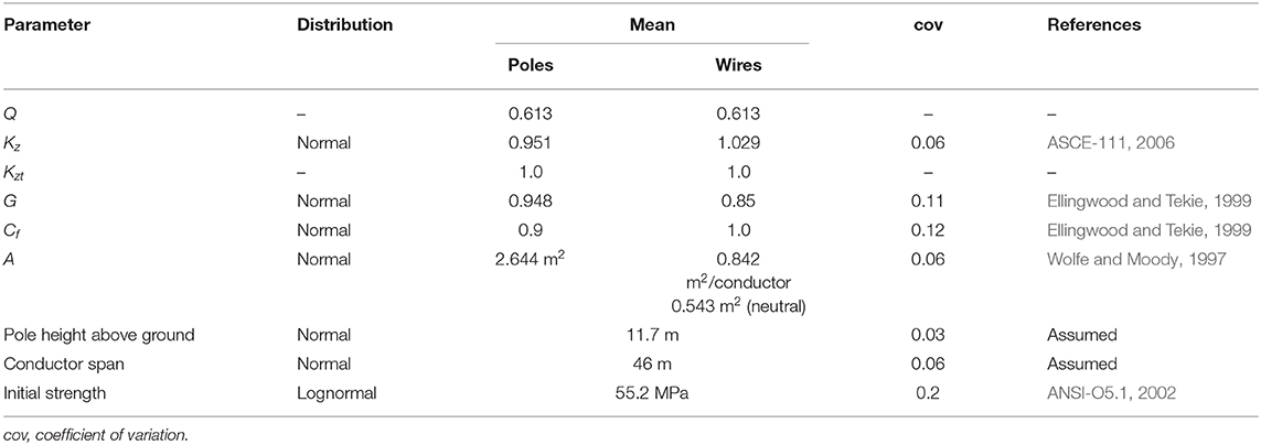
Table A1. Statistical parameters for fragility analysis.
Keywords: maintenance optimization, utility poles, hurricanes, climate change, power systems
Citation: Salman AM, Salarieh B, Bastidas-Arteaga E and Li Y (2020) Optimization of Condition-Based Maintenance of Wood Utility Pole Network Subjected to Hurricane Hazard and Climate Change. Front. Built Environ. 6:73. doi: 10.3389/fbuil.2020.00073
Received: 02 March 2020; Accepted: 27 April 2020;
Published: 22 May 2020.
Edited by:
Vagelis Plevris, OsloMet–Oslo Metropolitan University, NorwayReviewed by:
David De Leon, Universidad Autónoma del Estado de México, MexicoYou Dong, Hong Kong Polytechnic University, Hong Kong
Copyright © 2020 Salman, Salarieh, Bastidas-Arteaga and Li. This is an open-access article distributed under the terms of the Creative Commons Attribution License (CC BY). The use, distribution or reproduction in other forums is permitted, provided the original author(s) and the copyright owner(s) are credited and that the original publication in this journal is cited, in accordance with accepted academic practice. No use, distribution or reproduction is permitted which does not comply with these terms.
*Correspondence: Abdullahi M. Salman, ams0098@uah.edu