Molecular dynamics identifies semi-rigid domains in the PD-1 checkpoint receptor bound to its natural ligand PD-L1

1 Introduction

1.1 Medical background and clinical significance

Immune system T-cells detect cancer cells as they develop, and normally kill them (Smith-Garvin et al., 2009). However, some cancer cells have developed mechanisms to escape this important, immune–mediated clearance (Chen and Mellman, 2013) as follows: T-cells present a suicide tool (PD-1) on their surface. In healthy individuals, this tool is activated (by PD-L1) only if a T-cell should erroneously attack healthy tissue. PD-1 is therefore called an “immune-checkpoint”.

However, some cancer cells also express PD-L1 on their surface. They exploit the above checkpoint mechanism, abusively activate the immune checkpoint molecules (Dong et al., 2002) and thereby escape destruction. By increased expression of PD-L1 and/or the release of immunosuppressive factors cancer cells may survive even in a “hot”, immune-cell enriched surrounding.

Checkpoint inhibitors are drugs blocking the binding between PD-1 and its natural ligand, PD-L1. Clinical trials have proved their efficacy (Brahmer et al., 2012; Kwa and Adams, 2018). More recently a phase III trial in metastatic triple negative breast cancer patients showed a distinct improvement in progression-free survival and overall survival (Brahmer et al., 2018). This demonstrates the significance of the target (PD-1) being expressed when a PD-L1 antibody is used (Schmid et al., 2018; Cortés et al., 2019).

In order to further improve these promising therapies, a better understanding of the molecular mechanism of the PD-1 receptor is necessary.

1.2 Rationale for multi-level clustering

To evaluate minute movements within molecular dynamics trajectories, all frames need to be fitted to a certain intramolecular region (i.e. domain) at a reference frame (point in time). Such a fitting domain should not significantly deform itself over time (along a trajectory), in order to serve as a stable reference against which very small and intricate movement patterns outside this domain can be detected.

In previous work, domains for fitting were usually selected manually, based on secondary structure, such as beta-strands, beta-sheets or alpha helices. We detect such stable regions in an unsupervised procedure from the computed dynamics itself. In particular for example, if parts of beta-strands participate in the binding mechanics to be evaluated, they should not at the same time be part of the domain to which fitting is performed.

A most direct approach would be clustering according to small changes in distance between pairs of atoms over the whole trajectory. However, it is known that molecular systems tend to switch between metastable states, each of which may pertain over considerable parts of the simulation. During such a metastable state, some pairs of atoms might remain in close vicinity, with little variation of their distances. For example, atoms in some loop, which assumes a certain conformation characteristic for this and only this meta-state. Clustering only during this meta-state would send these pairs into the same cluster. However, as the system switches to another meta-state, the very same pairs of atoms could be detached from each other, become members of different neighborhoods and end up in different clusters if clustering would be performed only over this second meta-state. In consequence, one single pass of clustering over the whole trajectory might particularly conceal minute patterns of motion, being of focal interest. Separate clustering of segments of a trajectory is likely to take account of such minute differences between meta-states and exclude these regions from semi-rigid domains to be obtained.

Deriving rigidity directly and unsupervised from the simulation is considered a promising advantage and basis for future MD-studies.

1.3 Molecular structures

The molecular structure of the immune checkpoint PD-1 is shown in Figure 1, generated with VMD (Humphrey et al., 1996; Hsin et al., 2008; Cross et al., 2009) from PDB (Burley, 2013) entry 4ZQK (Zak et al., 2017). Since 4ZQK does not contain the complete structure of PD-1, we have modelled the missing parts in silico already in our previous work (Roither et al., 2021). The immune checkpoint receptor, PD-1, consists of several beta strands in tight mutual binding and respective loops in between, see Table 1. These loops protrude loosely from a rather compact beta core and offer versatile modes of interaction and binding. In particular, the residues 70 to 77, comprising the CC′-loop, are crucial for interaction with the natural ligand PD-L1 (Kundapura and Ramagopal, 2019), see Figure 2. Details of this interaction have been investigated experimentally by Zak (Zak et al., 2015) and in molecular dynamics studies by Liu (Liu et al., 2017) and our group (Roither et al., 2020; Tomasiak et al., 2020; Roither et al., 2021; Tomasiak et al., 2021).

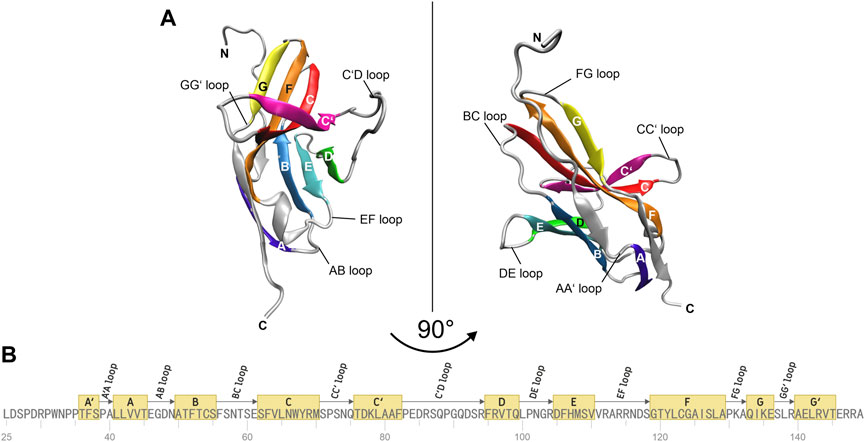
FIGURE 1. Molecular structure of immune checkpoint molecule PD-1. (A) Cartoon representation of the extracellular domain of PD-1. A two-layer β sandwich is formed by two β sheets GFCC’ (colored yellow, orange, red, magenta) and ABED (colored violet, blue, cyan, green) with loops connecting the respective β strands (colored silver). (B) Sequence of the residues of PD-1. The β strands of the protein are depicted as yellow boxes and the connecting loops as arrows. The figures were prepared using VMD version 1.9.3 (Humphrey et al., 1996).

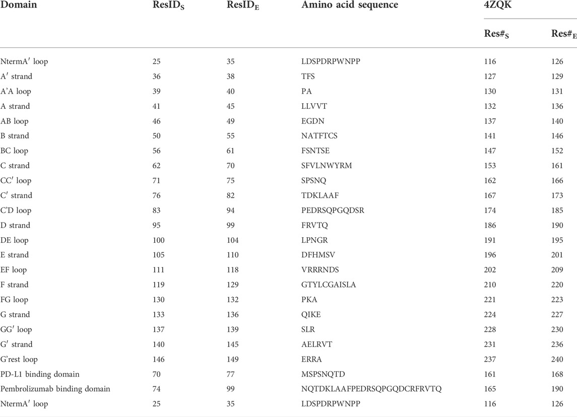
TABLE 1. Residues and secondary structure of PD-1. The assignment of strands and loops was chosen according to the classification of the Protein Feature View applet available within the 4ZQK record of the PDB. The domains were named following canonical Ig-strand designations (Zak et al., 2015). ResID_S and ResID_E indicate the starting and the ending residue ID of the according domain within chain B of 4ZQK. Res#_S and Res#_E indicate the starting and the ending residue number of a domain (continuous numbering for the whole complex in the respective PDB file).

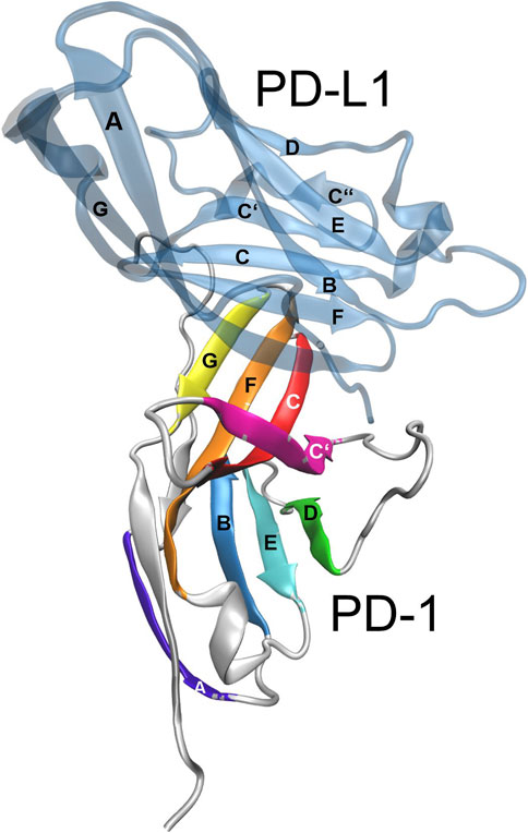
FIGURE 2. Immune checkpoint molecule PD-1 and binding partners. Cartoon representation of the extracellular domain of PD-1 bound to the endogenous ligand PD-L1 (transparent blue). The figure was prepared using VMD version 1.9.3 (Humphrey et al., 1996).

In the present work we draw on previous experience with the same system (Roither et al., 2020; Roither et al., 2021) but focus on unsupervised clustering, using a very efficient algorithm (Kenn et al., 2016) previously developed for MHC-molecules and T-cell receptors (Kenn et al., 2014).

2 Materials and methods

Molecular preparation and technical details of the molecular dynamics (MD) simulation have already been reported (Tomasiak et al., 2021). In Sections 2.1, 2.2, we briefly recapitulate essential points for completeness. The remaining subchapters Sections 2.3.1–2.3.5 refer to evaluation methods specific for this work.

2.1 Preparation of molecular complexes

Structural data for MD simulations were downloaded from the protein data bank (PDB, https://www.rcsb.org/) using the following entries: PDB-ID 4ZQK for the PD-1/PD-L1 system (resolution: 2.45 Å) (Zak et al., 2015) and PDB-ID 5GGS for the PD-1/pembrolizumab Fab fragment complex (resolution: 2.0 Å) (Lee et al., 2016). Missing residues in the crystal structure of the endogenous ligand PD-L1 in complex with the extracellular domain of PD-1 (PDB-ID 4ZQK), were added from the PD-1/pembrolizumab system (PDB-ID 5GGS), the N loop was taken from the PD-1/nivolumab system (PDB-ID 5WT9), see Roither et al. (Roither et al., 2020) for further preprocessing details. For determining the protonation states at pH 7.0 the H++ Server was used (http://biophysics.cs.vt.edu/) (Gordon et al., 2005). The assignment of strands, sheets, and loops was made following the classification of the Protein Feature View applet available within the 4ZQK record of the PDB (see Figure 1B).

2.2 All-atom molecular dynamics

As described previously (Tomasiak et al., 2021) all-atom MD simulations were performed with GROMACS 2021.2 (Hess et al., 2008), using the Amber99sb-ildn force field (Lindorff-Larsen et al., 2010) and an explicit water model. For the simulation box a rhombic dodecahedron was chosen with a minimum distance of 2 nm between the respective molecules and the box boundaries. The PD-1/PD-L1 complex consists of 4099 atoms and 240 residues, and the complex was solvated in TIP3P water (Jorgensen et al., 1983). Solute molecules were replaced by sodium and chloride ions to reach a physiological salt concentration of 0.15 mol/L.

For the energy minimization the method of steepest-descent was chosen. Before production runs the systems were equilibrated at NVT and NPT for 100 ps (time step 2 fs) each. In the NVT equilibration run the temperature was set to 310 K using a Berendsen-thermostat (Berendsen et al., 1984) with a time constant of 0.1 ps and position restraint MD. Equilibration in NPT ensembles was performed under the control of a Berendsen-barostat (Berendsen et al., 1984) set to 1 bar with a time constant of 1.0 ps.

All independent production runs had a simulation time of 600 ns with a time step of 2 fs using the LINCS algorithm (Hess, 2008) for constraining bonds to hydrogen atoms. For the van der Waals interactions a single cut-off of 1.47 nm was used and a cut-off distance of 1.4 nm for the short-range neighbor list in the Verlet scheme (Verlet, 1967) for neighborhood search. For electrostatic interactions the particle-mesh Ewald (PME) algorithm (Darden et al., 1993) was applied with a cut-off of 1.4 nm. Temperature coupling was done with the velocity-rescaling algorithm (Bussi et al., 2007) at a temperature of 310 K and for pressure coupling at 1 bar the Parrinello Rahman algorithm (Parrinello and Rahman, 1981) was used with a time constant of 2 ps. 30000 frames for each run were obtained by saving coordinates, velocities, forces, and energies every 20 ps to a trajectory file. Three independent 600 ns MD simulations with different initial velocities were carried out for each system, summing up to a total simulation time of 600 ns * 3 = 1.8 μs.

Prior to the evaluation, all frames of each given trajectory were fitted to the first frame of the trajectory, according to minimum root mean square deviation (RMSD) at time t. In mathematical terms, the Cartesian coordinates ${\mathbf{x}}_i$ of all atoms i were translated and rotated towards minimum RMSD of the backbone within β-strands and α-helices:

where x_i(t) is the position of atom i at time t. For the precise regions of secondary structure elements (β-strands and α-helices), see Tables 1, 2. N_bb is the total number of backbone atoms (N, C_α, C_O) contained therein. Finally, the first 100 ns of each trajectory were discarded to get rid of initial phase trends, leaving 500 ns with N_t = 25000 frames for each trajectory to be further analyzed.

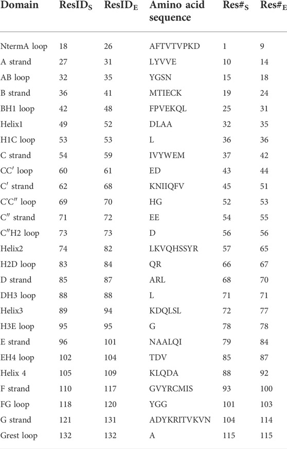
TABLE 2. Residues and secondary structure of PD-L1. The assignment of strands, loops and helices was chosen according to the classification of the Protein Feature View applet available within the 4ZQK record of the PDB protein data bank. The domains were named following canonical Ig-strand designations (Zak et al., 2015). Res#_S and Res#_E indicate the starting and the ending residue number of a domain (continuous numbering for the whole complex in the respective PDB file).

2.3 Obtaining semi-rigid domains

Semi-rigid domains for a given trajectory were obtained in a two-step process: First, “spatial clustering” was performed by grouping C_α-atoms showing similar movements into each of the clusters. Evidently, such a clustering does not need to (and will not) yield exactly the same clusters if spatial clustering is performed for different subsections of N_f frames each (called “segments” in the following) of a trajectory: Some pairs of C_αs will stay together in a given cluster over many segments, others will not (Kenn et al., 2014). This fact is exploited to perform “time-wise clustering” as a second step, by constructing new clusters from those C_αs which stay together within spatial clusters across successive segments with maximum fidelity. Such groups of atoms form clusters even more stable over time and are hence termed “semi-rigid domains” (Kenn et al., 2016). The total number of frames used from a trajectory, N_t, is partitioned into N_s segments, with N_t = N_s * N_f. We used N_s = 500 and N_f = 50, corresponding to 1 ns per segment and a frame length of 20 ps.

Note that time-wise clustering is a special mode of consensus clustering (Monti et al., 2003), since the same clustering algorithm is applied to different parts of a trajectory and a consensus between these results is finally adopted.

2.3.1 Spatial clustering

One crucial aspect of collective motion of atoms is captured by the variability (standard deviation) of mutual distances (Kenn et al., 2014), usually termed STDDV. We use it as an approximation for “motional distance” between two C_αs i and j, and denote it for brevity by D_ij defined as

where $d_{ij}=\Vert {\mathbf{x}}_i-{\mathbf{x}}_j\Vert$ is the Euclidean distance in a given (time-wise) frame and $\langle \rangle$ denotes averaging over all N_f frames for which clustering is intended, see Figure 3. Note that distances are not affected by any fitting of the trajectory to a reference frame.

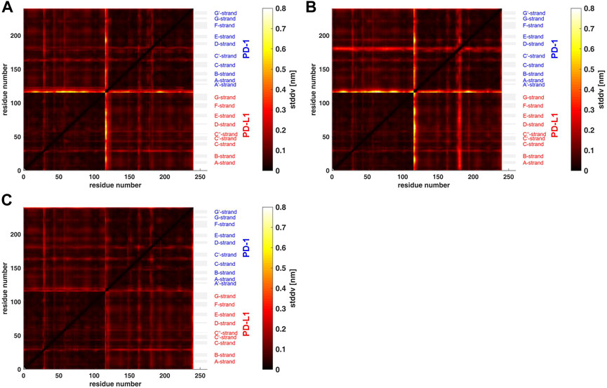
FIGURE 3. Matrix of standard deviations of atom distances over whole trajectories, shown as scaled color image (SCI). (A): Trajectory t₁ for complex 4ZQK, consisting of receptor PD-1 and PD-L1 as ligand, showing enhanced similarity within two large areas (receptor and ligand, respectively). Note that numbering starts with ligand PD-L1 with residue-ID = 18 (lower left corner), corresponding to residue number i = 1 in both axes of the SCI shown. PD-L1 extends over 1 ≤ i ≤ 115. The N-terminal end of PD-1 starts with residue-ID = 25 and extends over residues 116 < i < 240 towards the right upper corner. Elements of secondary structure are denoted right to the SCI (Zak et al., 2017), with their extensions indicated by horizontal grey shaded bars. Standard deviations D_ij [nm], computed according to Eq. 2, for values see color bar. (B): trajectory t₂. (C): trajectory t₃.

For actual spatial clustering (over segments or over the whole trajectory) we consider C_α atoms only and follow the concept of Bernhard and Noé (Bernhard and Noé, 2010). Each ${\mathrm{C}}_{\alpha ,i}$ is assigned a membership in cluster m, expressed as a real number $0\le c_{i,m}\le 1$, with zero meaning no membership and 1 standing for full membership. According to Bernhard and Noé, the N_α C_α atoms of the backbone are optimally decomposed into k clusters by minimizing the following target function:

In the formulation of Bernhard and Noé, memberships were assumed to be real numbers. This works successfully in the end but affords tremendous computational expense. In our previous work (Kenn et al., 2014) we were able to improve Bernhard’s and Noé’s method by showing mathematically that the membership coefficients, c_im, have in fact to be crisp, i.e., $\left\{\mathrm{0,1}\right\}$. Knowing this in advance drastically speeds up the minimization specified in Eq. 3. Since a given atom can only fully belong to one and only one cluster (no fragmentary membership), optimization can draw on single atom moves between clusters. We applied such a fast random search with single atom moves, followed by exhaustive searches to obtain a global optimum. Each lap of clustering was performed 100000 times and the result with the best target function retained. For computational details, parameter studies and thorough evaluations of accuracy and performance we refer to our previous work (Kenn et al., 2016).

As a result, spatial clustering yielded crisp memberships, $c_{i,m}^{\left(s\right)}=\left\{\mathrm{0,1}\right\}$, for C_α-atom i, in cluster m, within segment s, see Figure 4. Note that $1\le i\le N_{\alpha }$, $1\le m\le k$ and $1\le s\le N_s$.

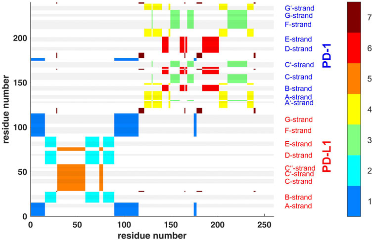
FIGURE 4. Clustering standard deviations of distance variation (STDDV) with k = 7 over the whole trajectory t₁. The best out of 100000 trials in the search for minimum target function is shown. Each cluster (1–7) is shown in a separate color, see the color bar. The sizes of clusters 1 to 7 were 44, 39, 39, 36, 34, 32 and 16. Elements of secondary structure are indicated by grey shaded bars and corresponding labels.

2.3.2 Time-wise consensus clustering

To arrive at a consensus we start with defining dissimilarity ${\Delta }_{ij}$ between two C_α -atoms i and j as:

with ${\Delta }_{ij}^{\left(s\right)}=0$ if atoms i and j belong to the same cluster $C_m^{\left(s\right)}$ in segment s and ${\Delta }_{ij}^{\left(s\right)}=1$ otherwise. Summing up ${\Delta }_{ij}^{\left(s\right)}$ over all segments (s) yields the number of segments within which i and j are not within the same cluster (Monti et al., 2003). Note that the number of segments is an upper bound, e.g. atoms i and j may reside “not in the same cluster” in 30 segments out of 500. The precise choice of segment length has only minor impact on the results. Shorter segment lengths (e.g., 25 frames per segment) yield a similarity matrix of higher resolution, but entails only minute changes in the final results. Naturally, a minimum length of segments is required to obtain a reliable estimate of variances. Division by the number of segments (N_s) finally renders a normalized measure of dissimilarity between i and j, relating to the whole trajectory (e.g., 30/500 = 0.06). This dissimilarity lends itself as a proxy for “distance” between atoms in this second lap of clustering (consensus clustering). Since cluster memberships are crisp, $c_{im}^{\left(s\right)}\in \left\{\mathrm{0,1}\right\}$, the concept above can also be expressed more formally (but less intuitively) via a product of memberships, see the second part of Eq. 4. Dual to dissimilarity, a similarity-matrix can be obtained via

see the example displayed in Figure 5. Note that similarity, as defined above, will be used synonymously with “consensus” in the framework of consensus clustering. Naturally, C_α atoms in close succession along the backbone appear close to the diagonal and show high consensus, see the color bar.

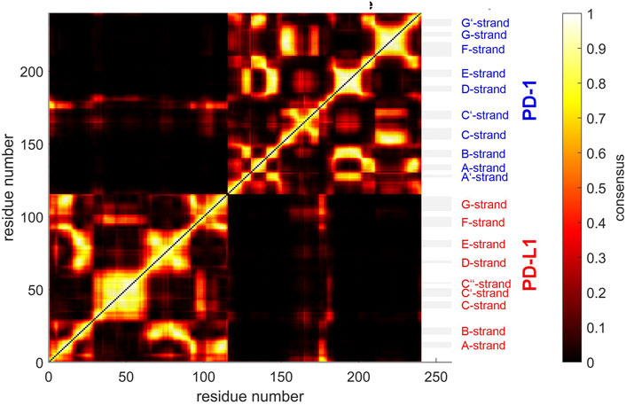
FIGURE 5. Similarity matrix after temporal consensus clustering trajectory t₁, shown as scaled color image (SCI). Complex 4ZQK, consisting of receptor PD-1 and PD-L1 as ligand, showing enhanced similarity within two large areas (receptor and ligand, respectively). Note that numbering starts with ligand PD-L1 with residue-ID = 18 (lower left corner), corresponding to residue number i = 1 in both axes of the SCI shown. PD-L1 extends over 1 ≤ i ≤ 115. The N-terminal end of PD-1 starts with residue-ID = 25 and extends over residues 116 < i < 240 towards the right upper corner. Elements of secondary structure are denoted right to the SCI (Zak et al., 2017), with their extensions indicated by horizontal grey shaded bars. Spatial clusters: 7. Note that the number of spatial clusters influences the similarity matrix and is given as input for computation. Consensus (0–500) indicates in how many (out of 500) timewise segments two C_α atoms belonged to the same spatial cluster (no matter which cluster that was). Consensus shown normalized to 0–1, see Eq. 5 and color bar.

Another very illustrative way to display consensus between atoms is a circular plot, see Figure 6. All C_α-atoms are arranged in a circle and a threshold, ${\Delta }_{\mathrm{t}\mathrm{h}}$, has to be chosen. Whenever the dissimilarity between two atoms is smaller than the threshold (${\Delta }_{ij}\le {\Delta }_{\mathrm{t}\mathrm{h}}$), these are connected by a line. Thus, connected atoms show small fluctuation in their distance over time.

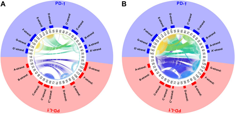
FIGURE 6. Circular plot of small variations of inter-atom distances for PD-1 complexed with PD-L1. Trajectory 2, spatial clusters k = 7. Residues numbered within each chain according to PDB convention. Around the circular plot, elements of secondary structure are indicated. Left: threshold for link to be drawn: ${\Delta }_{\mathrm{t}\mathrm{h}}=0.04=20/500$. Right: ${\Delta }_{\mathrm{t}\mathrm{h}}=0.1=50/500$.

2.3.3 Second lap of clustering based on consensus

The dissimilarity matrix ${\Delta }_{ij}$ was then subjected to agglomerative clustering (Ward, 1963; Jain et al., 1999), evaluating two methods for comparison, “average” and “complete” (Mathworks, 2021). They differ in their mode of linkage, i.e., the way, how the distance between two given (intermediate) clusters is computed: Method “average” takes the mean distance between individuals in different clusters to represent the distance between both clusters. Conversely, method “complete” adopts the largest of those between-cluster distances as the distance between the two clusters.

The methods “average” and “complete” are both appropriate for Euclidean as well as for non-Euclidean distances, which we worked with, after all. A third method (“single”) would also be appropriate for non-Euclidean distances, however it tends to yield a large number of small clusters, what seemed inappropriate for the structure of our molecules. Other methods are restricted to Euclidean distances.

Agglomerative clustering yields a tree-like-structure (dendrogram), an example is shown in Figure 7. At the left vertical axis C_α atoms are arranged and colored according to cluster membership, the residue-index being irrelevant here. The horizontal axis shows dissimilarity, in our case values between 0 (each C_α-atom against itself) and a maximum equal to the number of segments, N_s, into which the trajectory was split (e.g., 500). Note that this maximum applies to the methods chosen in this work but need not apply to other clustering methods, such as “Ward” for example.

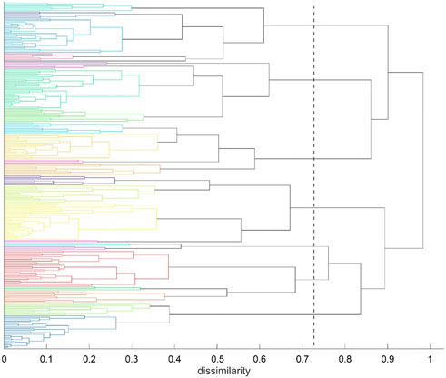
FIGURE 7. Agglomerative clustering according to inter-atomic time-wise consensus. Spatial clustering (k = 7 clusters) within each of 500 time-wise segments. Consensus among these 500 results of clustering was converted into distances and subjected to agglomerative clustering with distance model “average”. For reasons of clarity we call the results of agglomerative clustering “groups” in the following—to distinguish from the results of spatial clustering (“clusters”). Agglomerative clustering was terminated at N_G = 24 groups. The dashed line indicates N_G = 7 groups, as an example.

Clustering starts at bottom, with each atom representing a cluster of its own (leaves of the tree). Then clustering proceeds upwards (from left to right in Figure 7), in each step joining two clusters, selected among all pairs according to minimum distance. Note that there is no universal definition of “distance” between two clusters but one has to choose among several variants, i.e., “average” or “complete” in this work. Note that “distance” appears on the horizontal axes in Figure 7. As a result, any emerging cluster contains the sum of atoms contained in both of its predecessors. Finally, the algorithm terminates with a cluster containing all atoms, at the root of the tree.

The tree is then retraced from the root towards the leaves (from right towards left in Figure 7), along decreasing dissimilarity. Whenever a bifurcation is crossed, the number of clusters increases, one by one. One may proceed until a preselected number of clusters, N_C, is encountered (e.g. N_C = 7 in Figure 7) and thus obtain a corresponding ”cut-point” in terms of dissimilarity, see the dashed line. Quantitatively, the cut-point is computed as the median of those two levels of dissimilarity that have been passed though latest during recovery. In Figure 7, the final cut-point for display was selected at N_C = 24 groups (left, bottom border of tree). This number of clusters was chosen to accommodate several large, compact domains within the molecule (such as beta-sheets) as well as several smaller parts, such as freely moving loops. This intention has been fulfilled as clearly reflected in Figures 4, 8. These clusters represent a partition of all atoms into a given number (N_G) of groups $\left\{{\mathrm{G}}_1,{\mathrm{G}}_2...{\mathrm{G}}_{N_{\mathrm{G}}}\right\}$, as shown in Figure 9. These groups are shown in different colors.

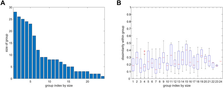
FIGURE 8. Number of atoms and variability of distance variation within groups from agglomerative clustering. 4ZQK, trajectory t₁, parameters k = 7 and N_G = 24, similar to Figure 7. (A) Size of group (number of atoms). (B) Homogeneity within groups shown by a boxplot of distance variations between pairs of atoms within each group (mean, quantiles, extremes).

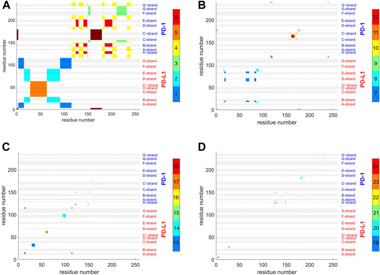
FIGURE 9. Atom groups resulting from agglomerative clustering consensus. 4ZQK, trajectory t₁, parameters k = 7, cutoff N_G = 24 groups. Note that the groups were internally numbered in order of descending size and each cluster is indicated by the color along the color bar to the right. To visually represent as many as 24 groups, 4 panels were generated for groups 1–6 (A), 7–12 (B), 13–18 (C) and 19–24 (D). Note also that each cluster does not need to appear as coherent field in the matrix, since remote atoms in the peptide chain may belong to one and the same cluster, as shown in the circular graph, Figure 6. To identify a single cluster, all fields of the same color within one given panel have to be considered together. All in all, the picture reflects the intricate connections of intra-molecular motions. Elements of secondary structure are indicated by grey shaded bars and corresponding labels.

2.3.4 Estimating the stability of clusters across trajectories

Above we have explained spatial clustering within consecutive segments of a single trajectory and then how to perform agglomerative clustering into domains, based on time-wise stability of these spatial clusters. Resulting clusters were called “semi-rigid”. Finally, we evaluate how much clusters differ between independent trajectories of the same molecular system. This comparison yields an estimate of cluster-stability on an upmost level, and was performed as follows.

For a trajectory t, N_G time-wise consensus clusters $\left\{{\mathrm{G}}_1^{\left(t\right)},{\mathrm{G}}_2^{\left(t\right)}...{\mathrm{G}}_{N_{\mathrm{G}}}^{\left(t\right)}\right\}$ were obtained, with $t=\mathrm{1,2,3}$, since three trajectories were generated. Let cluster-memberships of atom i in cluster m within trajectory t be denoted by $G_{im}^{\left(t\right)}=\left\{\mathrm{0,1}\right\}$, with $1\le i\le N_{\alpha }$, $1\le m\le N_{\mathrm{G}}$ and $1\le t\le 3$. When comparing results of agglomerative clustering between trajectories, the following problem arises: During agglomeration, emerging labels (identity numbers) of clusters may depend on minute, even somewhat random differences between trajectories. For example, if an existing cluster is to be joined with its “nearest” neighbor cluster, there might be two (or even more) neighbors almost equally “near”. As a consequence, even minute differences between trajectories in such a case induce different decision paths “which cluster wins”, and branch into different joining-operations for each trajectory. Since any new cluster generated (by joining) receives the next available cluster-label in sequence, a certain cluster-label may refer to two physically different groups of atoms in each trajectory. All in all, even though agglomerative clustering may produce nicely compatible physical groups of atoms, the labels of those groups might (and usually will) result totally permuted.

Therefore, after agglomerative clustering two trajectories, a so called “assignment problem” arises (Ramshaw and Tarjan, 2012): How should pairs of corresponding clusters be identified on an algorithmic basis?

In short, we proceeded as follows: We used the “Hungarian Algorithm”, drawing on the special target function given in Eq. 7. The value given by this target function represents the metric between trajectories. A vivid display is given in Figure 10, including a description how estimates come about for specific groups of C_α atoms.

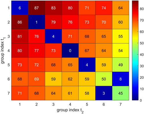
FIGURE 10. Visual representation of group-matching. Comparison of two sets of 7 C_α groups resulting for trajectory t₂ (horizontal axis) and trajectory t₁ (vertical axis). Group numbers are assigned with decreasing group size (7–1). Values given in matrix elements were evaluated via Eq. 6 and represent the loss function $L_{ij}^{\left(t_1,t_2\right)}$, i.e., the number of C_α atoms not contained in both groups. Low losses indicate good matching between groups and are colored blue, see the color bar. Diagonal elements represent a matching according to group size only, e.g., L₁₁ = 6 indicates that only 7 C_α atoms are not members of these both groups (1–1). Elements off the diagonal represent putative losses if group labels were permuted, e.g., L₁₂ = 87 indicates that 87 C_α atoms would mismatch in a putative comparison between group 1 from t₁ and group 2 from t₂. One can see that for groups 1 to 5, the original labelling (according to group size) is already optimum. Conversely, groups 6 and 7 have to be interchanged for optimum match.

In mathematical detail, the following procedure was performed: For each trajectory, NG (e.g., NG = 24) groups are obtained, and out of NG! possible pairings the best matching has to be determined, labels permuted accordingly, and re-assigned. Only on this basis, a comparison—cluster by cluster—is meaningful.

The assignment problem has been mathematically solved (Kuhn, 1955), based on the “Hungarian algorithm”, was put in a more general frame by Edmunds and Karp (Edmonds and Karp, 1972), and is now available in the MATLAB routine “matchpairs” (Duff and Koster, 2001): The user has to specify a so called “loss function” which quantifies the “loss” compared to a perfect match between two sets of clusters $\left\{{\mathrm{G}}_1^{\left({\mathrm{t}}_1\right)},{\mathrm{G}}_2^{\left({\mathrm{t}}_1\right)}...{\mathrm{G}}_{{\mathrm{N}}_{\mathrm{G}}}^{\left({\mathrm{t}}_1\right)}\right\}$ and $\left\{{\mathrm{G}}_1^{\left({\mathrm{t}}_2\right)},{\mathrm{G}}_2^{\left({\mathrm{t}}_2\right)}...{\mathrm{G}}_{{\mathrm{N}}_{\mathrm{G}}}^{\left({\mathrm{t}}_2\right)}\right\}$. Note that a comparison is feasible only if both sets contain the same number of clusters, N_G. For example, when evaluating the disparity between a pair of clusters $\left\{{\mathrm{G}}_i^{\left(t_1\right)},{\mathrm{G}}_j^{\left(t_2\right)}\right\}$, one may use the symmetric difference

as a proxy for a so called loss function, with | | meaning the number of elements in a group (cardinality). If both sets contain the very same atoms, the loss L = 0, if they do not share a single atom, the loss $L_{ij}^{\left(t_1,t_2\right)}=\left|{\mathrm{G}}_i^{\left(t_1\right)}\cup {\mathrm{G}}_j^{\left(t_2\right)}\right|$, i.e., it equals the total number of atoms in both groups. For intermediate cases, L represents the number of atoms contained in just one of both sets but not in the other (exclusive or-condition).

Solving the assignment problem allows to re-label clusters in a way that clusters with the same index go in pairs (common index m replaces i, j) and this pairing entails minimum overall loss. For this optimum assignment, losses are added over all clusters to obtain the total clustering disparity between both trajectories:

Note that the solution of the assignment problem is not commutative, i.e. $D^{\left(t_1,t_2\right)}\ne D^{\left(t_2,t_1\right)}$, i.e. it makes a difference in results which trajectory comes first. We shall call it “reference” in the following, e.g. trajectories t₂ and t₃ may be mapped on reference t_1.

Optimized re-assignment and joint labelling of clusters allows to boil down each cluster to its “stable kernel”, K_m, made up by those atoms belonging to the “same” cluster in all three trajectories considered:

Such kernels may be displayed within 3D representations of the molecular complexes.

2.3.5 Relating groups to molecular structures

For each atom i, its kernel-membership k_i is known, with $1\le k_i\le N_{\mathrm{G}}$. This allows for visualization of such groups within 3D representations of the molecular complex. From the memberships we generated Tcl-commands (Welch et al., 2003) to color these groups in VMD (Humphrey et al., 1996), see also the figures shown in the results section.

3 Results

3.1 Results for whole trajectories

Applying the methods explained above we obtained results for the complex 4ZQK (PD-1 + PD-L1). First, standard deviations D_ij of pair-distances were computed over each whole trajectory, with N_f = N_t in Eq. 2. Figure 3 shows the result for trajectories t₁, t₂ and t₃. Considerable differences between trajectories t₁, t₂ and t₃ can be seen.

Second, spatial clustering was performed over whole trajectories, see an example in Figure 4 for t₁ and k = 7. Note that clustering in any case assigns each atom to one of the clusters, even if its STDDV to quite many other atoms are large, see the conspicuous stripes in shiny yellow in Figure 3. As a consequence, clusters obtained this way inevitably also house atoms not intended to be parts of semi-rigid domains.

3.2 Results for segmental clustering

Next, time-wise clustering was performed. Figure 5 shows the similarity matrix with values between 0 and N_s, indicating how often time-wise consensus clustering found two C_α atoms within the same cluster. Note that clusters are neither numbered nor labelled in this step, i.e., they do not have unique identifiers related to their “inhabitants” in terms of physical atoms. For example, the pair of C_α,128 and C_α,237 may be together in cluster 4 in time-wise segment 129 and together in cluster 5 in time-wise segment 237. This would yield a consistency count of 2 (out of 500). Naturally, the number of segments, N_s, poses an upper limit of consistency, expressing that these two atoms were in the same cluster in all segments.

As consensus relates to linked mobility, most strong linkages were seen within each molecule (chain) of the complex, i.e., within PD-1 and within PD-L1. This resembles the fact that beta-strands cooperatively fold into beta-sheets, and corresponding atoms move in a more concerted way. However, some weaker linkage is also present between both molecules, see the parts in orange for residues of PD-1 towards multiple parts of PD-L1: these regions show consensus. A few C_α atoms at the start (i.e., the N-terminal loop) of the ligand even show close relation to this region of PD-1, with consensus around 0.8 (appearing yellow).

Posing a threshold on dissimilarity, e.g., ${\Delta }_{ij}\le {\Delta }_{\mathrm{t}\mathrm{h}}$, a circular plot can be obtained, see Figure 6. Pairs of atoms are connected by lines to indicate consensus if they appear in different clusters in a fraction of segments smaller than ${\Delta }_{\mathrm{t}\mathrm{h}}$. For example, selecting ${\Delta }_{\mathrm{t}\mathrm{h}}=0.06=30/500$, connects atoms only if they end up in different clusters in no more than 30 (time-wise) segments, out of 500. Naturally, the larger the dissimilarity threshold, ${\Delta }_{\mathrm{t}\mathrm{h}}$, is chosen, the more connection lines populate the circular plot. Moreover, weak similarities, such as those between PD-1 and PD-L1, become visible only if large dissimilarities are tolerated (right panel of Figure 6). They faint away in quite a large percentage of frames.

The above results display concordance (i.e., similarity in movements) between atoms, as it results directly from time-wise consensus clustering, based on pairs of C_α atoms. These pairwise results (consensus matrix) were subjected to a further step of analysis, agglomerative clustering, see Figure 7. Note that choosing a certain number of clusters, e.g. N_G = 24, does not change anything of the algorithm, it just defines the level of cutoff through the tree where splitting into groups is considered as result. Note that dissimilarities between clusters may well exceed the upper limit of dissimilarities ${\Delta }_{ij}$ between single atoms.

Clusters resulting from agglomerative clustering are different in size (number of atoms), see Figure 8. The box plot indicates variability within groups, based in the standard deviations of inter-atom distances used as the key target for spatial clustering. Groups from agglomerative clustering may also be displayed in matrix form, see Figure 9. Like in Figure 5, atoms are numbered consecutively, as they occur in the 4ZQK complex in PDB. Elements of secondary structure have been annotated to hint at possible relations to atomic mobility. In addition, these groups were visualized in circular graphs, see Figure 11.

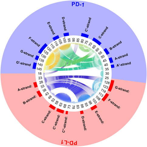
FIGURE 11. Circular graph of semi-rigid domains from agglomerative clustering time-wise consensus. 4ZQK, trajectory t₁, parameters k = 7, cutoff N_G = 24 groups. Connective lines colored according to C_α indices.

Agglomerative clustering starts with each atom representing its own cluster and then joins existing clusters. By proceedings upwards level by level, it creates a tree of larger and larger clusters, ending up in one maximum cluster above all others. This tree may be pruned at any level to yield different numbers of clusters. For comparison with clustering STDDV matrices according to Bernhard (Bernhard and Noé, 2010), see Figure 4, we display the agglomerative result pruned at N_G = 7, see Figure 12. Note that colors have been selected to match those of Figure 4, in order to be directly comparable.

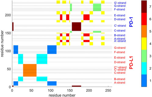
FIGURE 12. Atom groups for agglomerative clustering with cutoff N_G = 7 groups. Complex 4ZQK, trajectory t₁, parameters k = 7, cutoff N_G = 7 groups. For easy comparison with Figure 4, each cluster is shown in a separate color, see color bar. Colors were selected to match those of Figure 4, for direct comparison. Elements of secondary structure are indicated by grey shaded bars and corresponding labels.

3.3 Stability of clusters across trajectories

Note that all visualizations shown so far pertained to one single trajectory and a given set of clustering-parameters (k, N_G). It is interesting, however, to evaluate differences in results between trajectories. To these ends we utilized the disparity $D^{\left(t_1,t_2\right)}$ between pairs of trajectories, defined in Eq. 7. Discrepancies in agglomerative clustering between pairs of trajectories were 22, 40 and 28 for (t₁, t₂), (t₁, t₃) and (t₂, t₃), respectively (see Table 3). Comparing three trajectories naturally leads larger discrepancies. For comparison, we also added the results for agglomerative clustering in 7 groups, concordant with the preceding Bernhard-clustering. Note that considering more groups increases the chance for residues to switch between groups, and concomitantly discrepancy increases, however, for generating the final consensus, the more discrepant smaller clusters were disregarded, see below.

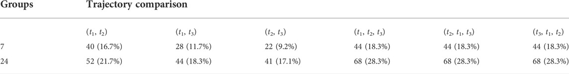
TABLE 3. Disparity in groups between trajectories. All results refer to k = 7 clusters for Bernhard clustering. Agglomerative clustering was performed for 7 and 24 groups, respectively. For each comparison between trajectories, discrepancies in agglomerative clustering are given as numbers of residues within different groups together with corresponding percentages of all residues (240). Note that, for a comparison between three trajectories (right part of table), disparities evaluated according to Eq. 7 depend on the choice of the reference trajectory, listed in position 1—as a coincidence, these results are all equal (44 and 68). Comparing 3 trajectories, means to include differences between 3 pairs of trajectories: For example, an atom counts as disparity if it resides in different clusters for (t₁, t₂) even if it resides in corresponding clusters in (t₁, t₃) and (t₂, t₃). As a consequence, disparities between triples of trajectories appear larger than those between pairs.

Finally, however, we also created a consensus between trajectories by estimating “kernels” of atoms belonging to the same cluster in all three trajectories, see Eq. 8. Note that the labelling of agglomerative groups originally varies randomly between trajectories and has to be consolidated as described in the methods section. Such a consolidated numbering—and a corresponding coloring—was used to outline the kernels within a 3D model of the molecular complex, see Figure 13. These kernels are considered as the “semi-rigid domains” aimed at.

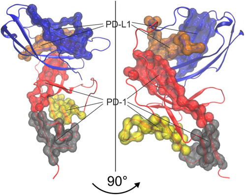
FIGURE 13. 3D-Visualization of semi-rigid domains resulting from spatio-temporal consensus clustering and consensus over trajectories. Groups obtained from agglomerative clustering were consolidated over 3 trajectories to obtain “kernels”, representing semi-rigid domains. The 5 largest kernels are colored and shown as surface representations. Note that kernels in red, grey and yellow belong to PD-1 while kernels in blue and ochre belong to PD-L1.

4 Discussion

We applied the method of spatio-temporal clustering to the PD-1/PD-L1 complex, aiming at identifying semi-rigid domains within these molecules. Such domains are considered a highly important basis for coming computational research since any detection of minute movement patterns requires to fit molecular configurations to stable kernels. Minute and interesting movement patterns, e.g., of active loops, may then be characterized with reference to such kernels.

During the course of an MD-simulation, larger portions (“domains”) of a molecule might collectively move slowly but move broadly back and forth in amplitude. Inside such a domain, however, single amino acids and even more single atoms oscillate at much higher frequencies. The goal is to separate these two types of movement occurring on different spatial and time scales: semi-rigid domains as a whole should go along with the larger but slower movements, while housing those many tiny oscillations of their “inhabitant“ atoms. As a result, a single atom performs both motions in superposition—small oscillations at high frequency, superimposed on larger and much slower collective motions of its corresponding domain. Both types of motion in combination influence the distances to its neighbor atoms.

In a non-supervised approach, one can only draw on the variation of distances as such, without knowing their origin (tiny oscillations of single atoms or large-scale movement of whole domains). Clustering atoms with respect to variations of pair-distances will therefore yield different results (clusters), when performed on different (time-wise) parts of a trajectory. Finally, however, a smart clustering algorithm should yield larger clusters “moving” in accordance with those larger domains, each of these holding much the same groups of atoms as inhabitants (members) over time.

For a start, we computed the standard deviations of distance variations (STDDV) matrices of whole trajectories (Figure 3). Since these matrices did not reveal prominent structures which could be clustered right away, we adopted a refined, three-step procedure. Moreover, distinct differences between trajectories became apparent in these matrices. We have to conclude that the system obviously inhabited different configurational sub-spaces in each trajectory, and simulation time has to be extended in coming studies to closer approach ergodicity and visit all portions of configuration space appropriately.

In the present work, matrices with different properties were studied. The STDDV-matrix does not reflect distances as such but rather variations in distance and therefore in general will not fulfil the triangle inequality. Incidentally, the Bernhard algorithm does not require fulfillment of the triangle inequality. In the second step of our algorithm we computed the dissimilarity matrix, Eq. 4, which fulfills the triangle inequality. This was a main reason for us to adopt this multi-step procedure.

To refine clustering we adopted a three-step procedure: First, clustering according to distance variation, but separately over short segments of the trajectory. Second, these results were consolidated over all segments of the trajectory by characterizing consensus for each pair of atoms: the percentage of time-wise segments in which these two atoms shared (resided in) the same cluster. Note that this second step yielded but pairwise information (consensus matrix), visualized in various forms (Figures 5, 6). Third, we performed agglomerative clustering to derive domain-like regions of coherence, the final result, shown in Figure 13. Note that cluster memberships after agglomerative clustering are in general different from those obtained by spatial clustering in the first lap.

The most intuitive approach would have been agglomerative hierarchical clustering, (Kaufman and Rousseeuw, 1990; Teukolsky et al., 2007). In a preliminary examination of the STDDV matrices (Figure 3) we found that an important precondition of agglomerative clustering is only poorly satisfied by MD data: Atoms may switch between clusters quite freely, without severely changing the target-function (minimum distance variability within clusters). This may easily deteriorate agglomerative clustering, and therefore we refrained from it as a first step. However, in future studies it would be interesting to mend this drawback, possibly by selecting more sophisticated models for linkage between clusters (others than “average” or “complete”). Also, agglomerative clustering allows to optimize the cut-off (i.e. the number of groups, N_G) according to formal criterions such as consistency (Mathworks, 2021). Linkage and cut-off could be systematically evaluated and optimized.

The achievement of the present work is the unsupervised consolidation of quite large domains within the molecular complex, despite considerable movements of its member atoms. Results were additionally consolidated by repeating the entire analysis for three independent trajectories and considering the overlap between these three replicates of a cluster as the final, reliable rigid domain. Based on these semi-rigid domains, subtle movements of active regions may be evaluated in future studies, scrutinizing the molecular basis of receptor activation and action of drugs, including checkpoint blockers in oncology.

Data availability statement

Publicly available datasets were analyzed in this study. This data can be found here: https://www.rcsb.org/structure/4ZQK, https://www.rcsb.org/structure/5GGS.

Author contributions

Conceptualization, WS, MK, HK, and GP; methodology, MK and RK; MD simulations, LT and RK; software, MK and MC; formal analysis and investigation, MK and WS; resources, HK; writing—original draft preparation, WS; writing—review and editing, WS, RK, and MK; visualization, LT, MC, and MK; supervision, WS. All authors have read and agreed to the published version of the manuscript.

Acknowledgments

A major part of the molecular dynamics computations for this work was performed at the Vienna Scientific Cluster (VSC).

Conflict of interest

GP received grants and honoraria from Pfizer, Roche, Novartis, MSD, Seagen, Daiichi, UCB, Amgen, AstraZeneca, and Gilead.

The remaining authors declare that the research was conducted in the absence of any commercial or financial relationships that could be construed as a potential conflict of interest.

Publisher’s note

All claims expressed in this article are solely those of the authors and do not necessarily represent those of their affiliated organizations, or those of the publisher, the editors and the reviewers. Any product that may be evaluated in this article, or claim that may be made by its manufacturer, is not guaranteed or endorsed by the publisher.

Supplementary material

The Supplementary Material for this article can be found online at: https://www.frontiersin.org/articles/10.3389/fbioe.2022.838129/full#supplementary-material

References

Berendsen, H. J., Postma, J. P. M., van Gunsteren, W. F., DiNola, A., and Haak, J. R. (1984). Molecular dynamics with coupling to an external bath. J. Chem. Phys. 81 (8), 3684–3690. doi:10.1063/1.448118
Bernhard, S., and Noé, F. (2010). Optimal identification of semi-rigid domains in macromolecules from molecular dynamics simulation. PLoS One 5 (5), e10491. doi:10.1371/journal.pone.0010491
Brahmer, J. R., Lacchetti, C., Schneider, B. J., Atkins, M. B., Brassil, K. J., Caterino, J. M., et al. (2018). Management of immune-related adverse events in patients treated with immune checkpoint inhibitor therapy: American society of clinical oncology clinical practice guideline. Jco 36 (17), 1714–1768. doi:10.1200/jco.2017.77.6385
Brahmer, J. R., Tykodi, S. S., Chow, L. Q., Hwu, W. J., Topalian, S. L., Hwu, P., et al. (2012). Safety and activity of anti-PD-L1 antibody in patients with advanced cancer. N. Engl. J. Med. 366 (26), 2455–2465. doi:10.1056/NEJMoa1200694
Burley, S. K. (2013). PDB40: The protein data bank celebrates its 40th birthday. Biopolymers 99 (3), 165–169. doi:10.1002/bip.22182
Bussi, G., Donadio, D., and Parrinello, M. (2007). Canonical sampling through velocity rescaling. J. Chem. Phys. 126 (1), 014101. doi:10.1063/1.2408420
Chen, D. S., and Mellman, I. (2013). Oncology meets immunology: The cancer-immunity cycle. Immunity 39 (1), 1–10. doi:10.1016/j.immuni.2013.07.012
Cortés, J., Lipatov, O., Im, S. A., Gonçalves, A., Lee, K. S., Schmid, P., et al. (2019). KEYNOTE-119: Phase III study of pembrolizumab (pembro) versus single-agent chemotherapy (chemo) for metastatic triple negative breast cancer (mTNBC). Ann. Oncol. 30, v859–v860. doi:10.1093/annonc/mdz394.010
Cross, S., Kuttel, M. M., Stone, J. E., and Gain, J. E. (2009). Visualisation of cyclic and multi-branched molecules with VMD. J. Mol. Graph. Model. 28, 131–139. doi:10.1016/j.jmgm.2009.04.010
Darden, T., York, D., and Pedersen, L. (1993). Particle mesh Ewald: An N⋅log(N) method for Ewald sums in large systems. J. Chem. Phys. 98 (12), 10089–10092. doi:10.1063/1.464397
Dong, H., Strome, S. E., Salomao, D. R., Tamura, H., Hirano, F., Flies, D. B., et al. (2002). Tumor-associated B7-H1 promotes T-cell apoptosis: A potential mechanism of immune evasion. Nat. Med. 8 (8), 793–800. doi:10.1038/nm730
Duff, I. S., and Koster, J. (2001). On algorithms for permuting large entries to the diagonal of a sparse matrix. SIAM J. Matrix Anal. Appl. 22 (4), 973–996. doi:10.1137/s0895479899358443
Edmonds, J., and Karp, R. M. (1972). Theoretical improvements in algorithmic efficiency for network flow problems. J. ACM 19 (2), 248–264. doi:10.1145/321694.321699
Gordon, J. C., Myers, J. B., Folta, T., Shoja, V., Heath, L. S., and Onufriev, A. (2005). H++: A server for estimating pKas and adding missing hydrogens to macromolecules. Nucleic Acids Res. 33 (2), W368–W371. doi:10.1093/nar/gki464
Hess, B., Kutzner, C., van der Spoel, D., and Lindahl, E. (2008). Gromacs 4: Algorithms for highly efficient, load-balanced, and scalable molecular simulation. J. Chem. Theory Comput. 4 (3), 435–447. doi:10.1021/ct700301q
Hess, B. (2008). P-LINCS: A parallel linear constraint solver for molecular simulation. J. Chem. Theory Comput. 4 (1), 116–122. doi:10.1021/ct700200b
Hsin, J., Arkhipov, A., Yin, Y., Stone, J. E., and Schulten, K. (2008). Using VMD: An introductory tutorial. Curr. Protoc. Bioinforma. 24, 51–55. doi:10.1002/0471250953.bi0507s24
Humphrey, W., Dalke, A., and Schulten, K. (1996). Vmd: Visual molecular dynamics. J. Mol. Graph. 14 (1), 3327–3838. doi:10.1016/0263-7855(96)00018-5
Jain, A. K., Murty, M. N., and Flynn, P. J. (1999). Data clustering. ACM Comput. Surv. 31 (3), 264–323. doi:10.1145/331499.331504
Jorgensen, W. L., Chandrasekhar, J., Madura, J. D., Impey, R. W., and Klein, M. L. (1983). Comparison of simple potential functions for simulating liquid water. J. Chem. Phys. 79 (2), 926–935. doi:10.1063/1.445869
Kaufman, L., and Rousseeuw, P. J. (1990). Finding groups in data: An introduction to cluster Analysis. New York: John Wiley.
Kenn, M., Ribarics, R., Ilieva, N., Cibena, M., Karch, R., and Schreiner, W. (2016). Spatiotemporal multistage consensus clustering in molecular dynamics studies of large proteins. Mol. Biosyst. 12 (5), 1600–1614. doi:10.1039/c5mb00879d
Kenn, M., Ribarics, R., Ilieva, N., and Schreiner, W. (2014). Finding semirigid domains in biomolecules by clustering pair-distance variations. BioMed Res. Int. 2014, 1–13. doi:10.1155/2014/731325
Kuhn, H. W. (1955). The Hungarian method for the assignment problem. Nav. Res. Logist. 2 (1-2), 83–97. doi:10.1002/nav.3800020109
Kundapura, S. V., and Ramagopal, U. A. (2019). The CC′ loop of IgV domains of the immune checkpoint receptors, plays a key role in receptor:ligand affinity modulation. Sci. Rep. 9 (1), 19191. doi:10.1038/s41598-019-54623-y
Kwa, M. J., and Adams, S. (2018). Checkpoint inhibitors in triple-negative breast cancer (TNBC): Where to go from here. Cancer 124 (10), 2086–2103. doi:10.1002/cncr.31272
Lee, J. Y., Lee, H. T., Shin, W., Chae, J., Choi, J., Kim, S. H., et al. (2016). Structural basis of checkpoint blockade by monoclonal antibodies in cancer immunotherapy. Nat. Commun. 7, 13354–13364. doi:10.1038/ncomms13354
Lindorff-Larsen, K., Piana, S., Palmo, K., Maragakis, P., Klepeis, J. L., Dror, R. O., et al. (2010). Improved side-chain torsion potentials for the Amber ff99SB protein force field. Proteins 78 (8), 1950–1958. doi:10.1002/prot.22711
Liu, W., Huang, B., Kuang, Y., and Liu, G. (2017). Molecular dynamics simulations elucidate conformational selection and induced fit mechanisms in the binding of PD-1 and PD-L1. Mol. Biosyst. 13 (1742-2051), 892–900. (Electronic)). doi:10.1039/c7mb00036g
Monti, S., Tamayo, P., Mesirov, J., and Golub, T. (2003). Consensus clustering: A resampling-based method for class discovery and visualization of gene expression microarray data. Mach. Learn. 52 (1-2), 91–118. doi:10.1023/A:1023949509487
Parrinello, M., and Rahman, A. (1981). Polymorphic transitions in single crystals: A new molecular dynamics method. J. Appl. Phys. 52 (12), 7182–7190. doi:10.1063/1.328693
Ramshaw, L., and Tarjan, R. E. (2012). On minimum-cost assignments in unbalanced bipartite graphs. HP Laboratories.
Roither, B., Oostenbrink, C., Pfeiler, G., Koelbl, H., and Schreiner, W. (2021). Pembrolizumab induces an unexpected conformational change in the CC′-loop of PD-1. Cancers 13 (1), 5. doi:10.3390/cancers13010005
Roither, B., Oostenbrink, C., and Schreiner, W. (2020). Molecular dynamics of the immune checkpoint Programmed Cell Death Protein I, PD-1: Conformational changes of the BC-loop upon binding of the ligand PD-L1 and the monoclonal antibody nivolumab. BMC Bioinformatics 21 (17). doi:10.1186/s12859-020-03904-9
Schmid, P., Cortes, J., Bergh, J. C. S., Pusztai, L., Denkert, C., Verma, S., et al. (2018). KEYNOTE-522: Phase III study of pembrolizumab (pembro) + chemotherapy (chemo) vs placebo + chemo as neoadjuvant therapy followed by pembro vs placebo as adjuvant therapy for triple-negative breast cancer (TNBC). Jco 36 (15), TPS602. doi:10.1200/JCO.2018.36.15_suppl.TPS602
Smith-Garvin, J. E., Koretzky, G. A., and Jordan, M. S. (2009). T cell activation. Annu. Rev. Immunol. 27, 591–619. doi:10.1146/annurev.immunol.021908.132706
Teukolsky, S. A., Vetterling, W. T., and Flannery, B. P. (2007). “Section 16.4. Hierarchical clustering by phylogenetic trees,” in Numerical recipes: The art of scientific computing. 3 ed (New York: Cambrige University Press), 701–744.
Tomasiak, L., Karch, R., and Schreiner, W. (2020). “Long-term molecular dynamics simulations reveal flexibility properties of a free and TCR-bound pMHC-I system,” in 2020 IEEE international conference on bioinformatics and biomedicine (BIBM), 1295–1302. doi:10.1109/bibm49941.2020.9313545
Tomasiak, L., Karch, R., and Schreiner, W. (2021). “The monoclonal antibody pembrolizumab alters dynamics of the human programmed cell death receptor 1 (PD-1),” in 2021 IEEE international conference on bioinformatics and biomedicine (BIBM), 3315–3321. doi:10.1109/bibm52615.2021.9669720
Verlet, L. (1967). Computer "experiments" on classical fluids. I. Thermodynamical properties of Lennard-Jones molecules. Phys. Rev. 159 (1), 98–103. doi:10.1103/PhysRev.159.98
Ward, J. H. (1963). Hierarchical grouping to optimize an objective function. J. Am. Stat. Assoc. 58 (301), 236–244. doi:10.1080/01621459.1963.10500845
Welch, B. B., Jones, K., and Hobbs, J. (2003). Practical programming in tcl/tk. Upper Saddle River, NJ: Prentice Hall Professional.
Zak, K. M., Grudnik, P., Magiera, K., Dömling, A., Dubin, G., and Holak, T. A. (2017). Structural biology of the immune checkpoint receptor PD-1 and its ligands PD-L1/PD-L2. Structure 25 (8), 1163–1174. doi:10.1016/j.str.2017.06.011
Keywords: molecular dynamics, checkpoint inhibitor, immune therapy, oncology, drug design, cluster analysis
Citation: Kenn M, Karch R, Tomasiak L, Cibena M, Pfeiler G, Koelbl H and Schreiner W (2022) Molecular dynamics identifies semi-rigid domains in the PD-1 checkpoint receptor bound to its natural ligand PD-L1. Front. Bioeng. Biotechnol. 10:838129. doi: 10.3389/fbioe.2022.838129
Received: 17 December 2021; Accepted: 14 September 2022;
Published: 06 October 2022.
Edited by:
Andrea Banfi, University of Basel, SwitzerlandReviewed by:
Andras Szilagyi, Institute of Enzymology, HungaryFátima Alejandra Pardo Avila, Stanford University, United States
Copyright © 2022 Kenn, Karch, Tomasiak, Cibena, Pfeiler, Koelbl and Schreiner. This is an open-access article distributed under the terms of the Creative Commons Attribution License (CC BY). The use, distribution or reproduction in other forums is permitted, provided the original author(s) and the copyright owner(s) are credited and that the original publication in this journal is cited, in accordance with accepted academic practice. No use, distribution or reproduction is permitted which does not comply with these terms.
*Correspondence: Wolfgang Schreiner, wolfgang.schreiner@meduniwien.ac.at