Predicting the data structure prior to extreme events from passive observables using echo state network

Introduction

In recent years, extreme events (EEs) have gained attention of the researchers and decision-makers due to increase in the occurrence of highly intense climate extremes, such as hurricanes, floods, heatwaves, etc., due to global warming and climate change [1–3]. They have devastating impact on life and infrastructure. There are several other examples of such extraordinary devastating events in various other disciplines aside from climate, like rogue waves in lasers and tsunamis in the ocean, earthquakes in seismology, share market crashes in finance, regime shift in ecosystems, etc., which are also rare but may have a long-term correlation in their return periods [4–11]. The study of extreme events focuses on the self-organizing principles [5, 12–19] that may enable us to forecast and mitigate the after effect. Various tools have been developed to study the underlying dynamics of such extreme events, e.g., complex networks have been extensively used to analyze climate extremes [20–24], numerous studies have been conducted to analyze extreme events based on their statistical properties [25, 26]. Recurrence plot analysis has been used to study the recurring behavior of flood events [27]. Because of their rare occurrence and complex dynamics, understanding and predicting extreme events is a challenge in the studies of complex natural systems using the dynamical system approach only [15, 28–30]. Alternatively, data-based and model-free machine learning techniques have been recently shown to be more promising for predicting such events [31–36]. To put it simply, such a prediction process involves training of the machine using past data records of EEs from other observable and then testing the ability of machine to successfully predict the prior shape of the observable which leads to extreme event.

As the term “extreme event” is used in various disciplines, a precise definition of EEs is not available. Rather, it depends on the particular discipline where this term is being used. In this work, we select the EEs based on their magnitude. Therefore, it is crucial to set a threshold height so that we can call an event “extreme” when it exceeds the threshold. The choice of an appropriate threshold plays a pivotal role in prediction [37, 38]. In our study, we found that for data-based machine learning, a certain threshold height augments the efficient detection of the arrival of a coherent pattern and thereby leverage the prediction process. In particular, we raise the following question here that for a given multivariate data set in which one of the variables exhibits EEs, whether a seemingly benign variable (with no signature of EE) can be used in a machine for the prediction of the preceding structure or pattern indicative of the forthcoming EE expressed in another observed variable. We refer to the preceding structure pattern as a precursory signal in the data that is typically correlated with the occurrence of EE in near future. For example, farmers anticipate rain when they observe red clouds in the early morning sky.

The aforementioned question is motivated from the fact that the occurrence of EEs in one variable are a manifestation of the rich dynamics of a multivariate higher dimensional system as caused by the non-linear interactions among its various constituents [5, 13]. Due to the paucity of observations of some EEs occurring in nature, collection or reconstruction of data directly from a dynamic variable that flares up with an extreme value (active variable) such as the extreme precipitation, over a long time period is seldom possible. It is easier to reconstruct data for those observables which are slow varying (temperature, pressure, etc.). Some of these observables may remain silent or passive with a weak response and do not show up with any manifestation of large size extreme value. However, such passive variables carry significant information related to the EEs. We emphasize here that the data collected from the passive variable is used as inputs to a reservoir computing machine, i.e., the echo-state network (ESN), in order to check how efficiently the machine can capture the a priori structure in the active observable that precedes the EE. ESN is a simple version of recurrent neural networks [39] that has been used extensively to predict complex signals ranging from time series generated from chaotic model, stock-price data to tune hyperparameter [40–50]. Recently, it has been shown that ESN can efficiently capture the onset of generalized synchronization [51–55], quenching of oscillation [56, 57], detect collective bursting in neuron populations [58], and predict epidemic spreading [59]. ESN has been shown to have great potential in handling multiple inputs of temporal data, and ability to trace the relation between them [52, 58, 60]. Due to its simple and computationally effective character and its suitability for dynamical systems, we use ESN for our study. Other machine learning-based methods, such as deep learning [61] might also be useful for the problem we address in this work.

While collecting data, the first important task is to detect the EE by assigning an appropriate threshold height and collect a number of data segments prior to all the available EE in a time series, to address the question of predictability as suggested earlier [38, 62, 63]. In the present work, we rely on data generated from numerical simulations of a model system for training and testing of the ESN for efficient detection of the structure preceding the extreme events. Firstly, we identify a large number of visible EEs from the active variable using a threshold height and save a data segment of identical length prior to the occurrence of each EE from the active variable along with the corresponding data segment from the passive variable. A multiple number of data segments of identical length corresponding to EEs in the active variable are thus collected from the passive variable and used as inputs to the machine. A part or fraction of the data points from each segment is used for training and the rest of the data points is kept aside for predicting the preceding structure of EE in the active variable during testing.

We repeat the whole process of data collection, training and testing of the machine by varying the choice of the threshold height and then make a quantitative comparison based on predictability skill to select the most suitable threshold height for detection and prediction of EE. It must be noted that by prediction we imply the identification of a common pattern or structure in the test signal that always appears quite ahead of time before the arrival of extreme events and hence, effectively works as a precursor to the extreme events. Our machine learning based recipe unfolds two useful information: (i) Data collected from a passive variable before the appearance of EE in an active variable can provide clues to capture the future trend of an active variable and thereby predict the precursory shape of the forthcoming EE, (ii) machine can efficiently suggest a choice of appropriate threshold height that may augment the prediction process. A possible reason for the necessity of a critical threshold for accurate prediction by the machine is explained further in light of a coherent pattern that always appears in the ensemble of multiple segments of data inputs that has been collected prior to the EE.

For demonstration purpose, we use a paradigmatic model neuron that consists of active variables (fast variables) expressing the triggering of extreme events when its passive counterpart (slow variable) shows no signature of extremes.

Methodology

Dataset

For data generation of EEs, we numerically simulate a synaptically (chemically) coupled slow-fast Hindmarsh-Rose (HR) neurons model [64],

where x_i and y_i (i, j = 1, 2; i≠j) are the fast variables and oscillate with firing of spiking or bursting potentials. The slow variable z_i controls the fast oscillations. Each variable has its specific biological functional meaning. The system parameters a, b, c, and s are appropriately chosen where r < 1 is the slow parameter. x_R and v_s are constant biases and $\text{Γ}(x)=\frac{1}{1+e^{-\lambda (x-\Theta )}}$ is a sigmoidal function, typically used [65] to represent chemical synaptic coupling. The parameters, a = 1, b = 3, c = 1, κ = 5, x_R = −1.6, ρ = 0.01, s = 5, I = 4, v_s = 2, λ = 10, Θ = −0.25, are kept fixed for generating data. The coupling constant θ_{1, 2} decides the strength of mutual communication between the neurons via chemical synapses. We collect data on x_i and z_i (i = 1, 2) from numerical simulations and define two new variables, u = x₁+x₂ and v = z₁+z₂. Extreme events are expressed [65] in the fast variable u, which is denoted as our active variable, while the slow variable v is defined as the passive variable. The passive variable does show a signature of rising amplitude when extreme events arrive in the active variable. However, we have to make a cut-off in the range of the threshold as usually used from 4σ to 8σ in the literature. The rising peaks in the slow variable are not significantly large than our considered significant height (3.5σ to 6σ). Our motivation is to predict the precursory structures for rare peaks, and for this purpose, we consider the v variable as a passive variable. Information from the passive variable v is then used as input data to the machine for predicting the preceding structure of extremes in u.

The local maxima of a time series are identified as events and accordingly all the events are extracted from u for a long run. A standard definition is used for the identification of an extreme event [14, 15, 66] with a threshold H_s = 〈μ〉+dσ, where 〈μ〉 is the mean of the time series, σ is the standard deviation and d is a constant. Any event larger than H_s is considered as an extreme where d is allowed to vary from system to system or for a measured time series under consideration. The question of prediction and enhancing predictability is addressed here by setting different threshold limits of H_s by varying d.

For the purpose of numerical experimentation, we first detect a number of extreme peaks n from a long time series of u (total length of the time series : 2 × 10⁷) that crosses a predefined threshold H_s for a particular choice of d. Next, we collect k data points prior to each of the n peaks from u, i.e.,

where û₁, û₂, ..., û_n are the n events selected from active variable u. We also collect the corresponding data points from the v-time series, i.e.,

In other words, we collect n time segments each containing k data points prior to all the n extreme events, and construct a matrix called event matrix E of size n×k from the active variable and, similarly, construct a matrix P of the same size n×k by storing the corresponding data points from the passive variable. A set of m (m<n) (gray region A in Figure 2A) time segments each with data points p (p<k) (Figure 2B) as collected from v is then fed into the machine for training to predict the preceding structure of (n−m) segments in u signals (light red region B in Figure 2), which is considered as a precursor to the arrival of extreme events later. How the machine extracts information from the inputs of v and transforms them into u at the output is defined in the input-output functional relation of the machine as a description of the ESN in the next section. Once the training is over, the rest of the (k−p) data points for each of the m time segments are used for testing whether the machine can predict the future structure of (n−m) time segments of u. The whole process is repeated multiple times by using four different choices of d (3.5, 4, 5, 6) for detecting extremes from the time series of u. We emphasize once again that an input to the machine for training and testing consists of multiple segments of data points of identical length collected from v corresponding to the successive number of EE detected in u for each d-value. The data points collected from u are used at a later stage for comparison with the machine output during the testing process. Certainly this recipe works only when certain amount of data prior to the extreme events is available from both the variables, and the passive variable of the system can be identified. However, the advantage of such a methodology is that it is data-driven and model-free.

Reservoir computing: Echo-state network model

An echo state network (ESN) is a type of recurrent neural network and is extensively used due to its simple architecture [39]. It has three parts—(1) input layer—in which the weights are randomly chosen and fixed, (2) reservoir or hidden layer—it is formed by randomly and sparsely connected neurons and (3) output layer—in which the output weights are the only trainable part by input data. A standard leaky network with a tanh activation function is considered here as the ESN. The dynamics of each reservoir node is governed by the following recursive relation:

where r(t) is a n_res-dimensional vector that denotes the state of the reservoir nodes at time instant t, v(t) is the m-dimensional input vector and 1 is the bias term. The matrices W_res (n_res×n_res) and W_in (n_res×(m+1)) represent the weights of the internal connection of the reservoir nodes and weights of the input, respectively. The parameter α is the leakage constant, which can take any values between 0 to 1. It is to be noted that the tanh function operates element-wise. The choices of α and n_res can be varied. Here, we have fixed α = 0.6 and n_res = 600 throughout all simulations. The reservoir weight matrix W_res is constructed by drawing random numbers uniformly over an interval [−1, 1] and the spectral radius of the matrix W_res is re-scaled to less than unity. The elements of the input weight matrix W_in are also generated randomly from the interval [−1, 1]. Next we consider data of n-segments sequentially from the time series of v corresponding to n extreme peaks in u from which a set of first m-segments of length p of the total length of k data points are fed into the ESN for training. Thereafter, the output weight W_out is optimized to capture the trend of the (n−m) segments (each length: (k−p)) of u signals. Once the machine is trained, the input of m-segments each with (k−p) data points are fed into the machine to predict the trend of the (n−m)-segments of the u signals prior to the arrival of EE in time. At each instant of time t, the m−dimensional input vector of data, v(t):${\left[v_1(t),v_2(t),...,v_m(t)\right]}^T$ is fed into m-number of input nodes of the machine when the contribution of the input weight matrix in the dynamics of the reservoir (see Equation 4) is written as

During the training process, at each time instant t, the reservoir state r(t) and input v(t) are accumulated in V_train(t) = [1;v(t);r(t)]. The matrix V_train having dimension (n_res+m+1) × p look like,

The output weight is determined by:

where U_train is a matrix which stores the value of u from (n−m) segments of training length p, and λ = 10⁻⁸ is the regularization factor that avoids over-fitting. Now, the output weight is optimized, the final output is obtained by,

An important point to note is that we use the information of u only to optimize the output weight.

Results

For illustration of our proposed scheme, the original time series of u and v for a long run of numerical simulations are plotted in Figure 1A. As the threshold height is increased from H_s1 = 〈μ〉+3.5σ and H_s2 = 〈μ〉+6σ by varying d from 3.5 to 6, many large peaks are filtered out that declares only a few peaks as rare and extremes. The extreme peaks are selected as those which are higher than a selected threshold height H_s (horizontal line, Figure 1A) for a particular choice of d, and used as data for training and testing the reservoir shown in Figures 2B–D. It is clear that some of the peaks in u are higher than the designated thresholds H_s1 and H_s2 whereas the height of all the peaks in v are lower than both thresholds. A zoomed version is shown in Figure 1B to demonstrate the time evolution of u and v around a single extreme peak marked by a shaded region in Figure 1A. Extremes are only expressed in the active variable u with no similar manifestation in the passive variable v, which is considered here as the input candidate to the machine for the prediction of the a priori structure of successive EEs in u.

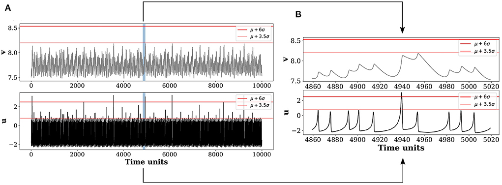
Figure 1. Time series of slow variable v and fast variable u of the coupled Hindmarsh-Rose (HR) system. (A) Horizontal red lines in the time series of u (lower panel) and v (upper panel), indicate two threshold heights H_s1 = 〈μ〉+3.5σ (thin line), H_s2 = 〈μ〉+6σ (bold line); μ and σ are the mean and standard deviation of the time series, respectively. Threshold height H_s2 filters out many large peaks that are otherwise qualified as extremes by the lower threshold H_s1, and thereby allows a selection of rarer extreme events only. One particular extreme peak (shaded region) is marked in (A) as shown in u, and zoomed in the lower panel of (B) for illustration. This extreme peak is larger than both the horizontal lines H_s1 and H_s2 so as to qualify as a rare extreme event. The corresponding part of the time series of the slow variable v in the upper panel of (A) that never crosses either of the thresholds, H_s1 and H_s2, is zoomed in and shown in the upper panel of (B). Although a slight increase in size of the peak is seen (B) compared to its neighboring peaks (upper panel), there is not much significant change in height in comparison to the extreme peak observed in u in the lower panel.

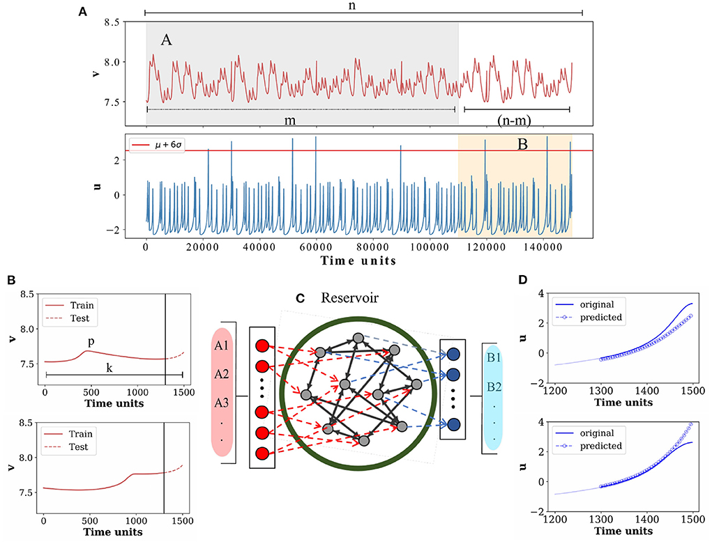
Figure 2. Schematic diagram of the ESN and the prediction process. (A) Time series of the passive variable v (upper panel) and active variable u (lower panel) with a number of extreme events, here selected using a threshold height H_s = μ+6σ, are shown. Data points (k = 1, 500) from v, and u prior to n extreme peaks are saved. A few exemplary extreme peaks are shown for demonstration. For our proposed scheme, data points around such n = 200 extreme peaks are collected. (B) Two exemplary input signals corresponding to two extreme events are shown here, while the actual number of input signals are m = 180 as for the training purpose. For each input node, p = 1, 300 data points (solid red line) are used for training purpose and the rest of (k−p) = 200 data points (dotted red line) are used for testing, which are separated by a vertical line (black line). (C) Echo state network structure: input layer consists of A_m nodes, where m = 180 input signals (data segments prior to each of the extreme events) are used for training. The output layer consists of B_n−m = 20 nodes. (D) Preceding pattern of predicted u signals from 20 nodes each for (k−p) = 200 datapoints (blue circles) and the original u signal (blue line) for 200 datapoints are plotted for comparison. Two such output signals are shown as examples.

An exemplary predicted output of u for (k−p) = 200 data points (blue circles) vis-à-vis the original u signal of the same length (blue line) is plotted in Figures 3A–D for four different d-values. A visual impression provides a clear evidence that the error between the predicted signal (blue circles) and the original input signal (blue line) during 1, 300 to 1, 500 time units decreases with the increase in the value of d. For a more comprehensive understanding of the scenario, the root mean square error (RMSE) estimated for 20 predicted output signals and the original signals of u is plotted which confirms the increasing predictability with higher H_s (Figures 3E–H). To verify the robustness of the outcome, we repeat the whole process for 400 realizations drawn from 400 different initial conditions. RMSE is calculated as follows:

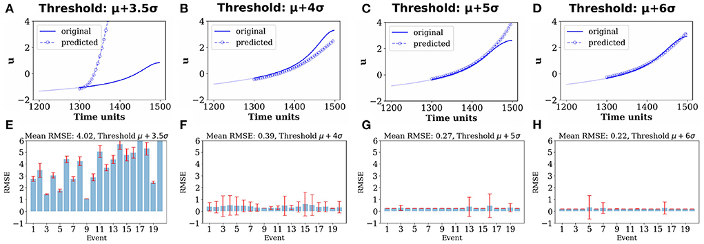
Figure 3. Prediction of extreme events by the ESN. Upper panels in (A–D) show original active signal u for (k−p) = 200 data points (blue line) along with the predicted signal for (k−p) = 200 data points (blue circles) for comparison for EEs selected using four different threshold heights computed using: (A) d = 3.5, (B) d = 4, (C) d = 5, and (D) d = 6. It shows an increased resemblance between the predicted and original extreme peaks with increasing d. Lower panels in (E–H) show RMSE between the original signal u and their predicted signals for (k−p) = 200 data during testing, estimated over 20 extreme events, corresponding to (A–D), respectively. Results of 400 realizations of data from numerical simulations of the model using 400 different initial conditions for each d-value are presented in (E–H) and the vertical bars mark their standard deviation.

where t_r and t_f are training and final time respectively and t_f−t_r = k−p.

To understand the reason for the machine's improved performance with higher a H_s, we compare all the 180 input signals of the passive variable (v) as well as the active variable (u) prior to the occurrence of EEs (p = 1, 300 data points) (Figure 4). Upper row plots in Figures 4A–D represent the input signals v before the EEs for four different threshold values. As we increase the threshold H_s (by increasing d from 3.5, 4, 5, 6), signals observed to get less dispersed and tend to form a coherent bundle.

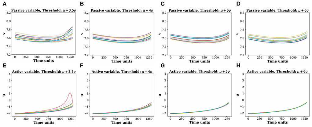
Figure 4. Comparative picture of coherence in the input time signals (p) extracted before an extreme events. (A–D) Input signal of passive variable v for threshold values (d = 3.5, 4, 5, 6). (E–H) are the corresponding active variable u for threshold values (d = 3.5, 4, 5, 6). Coherence between the input time signals increases with the threshold height determined by higher d-values. Different color signifies different trajectories.

In fact, the increasing coherent pattern among the input signals is more prominent in the corresponding active variable u in the lower row of Figures 4E–H than the v variable. For the highest threshold value, the time signals are almost coherent similar to what was reported by [62], where they showed the formation of coherent structure before the arrival of extreme events in the active variables. The increasing coherence in v with higher H_s enhances the machine's predictability skill for higher amplitude events compared to the lower amplitude ones. Thus, the machine establishes a general fact, in quantitative terms, that predictability is enhanced for larger value of threshold height when the input signals are more coherent for a longer duration of time [62, 63].

We repeat our experiments using the same ESN by considering two different length of data inputs (p = 800, 1, 300) prior to each of the extreme events for training, and keeping the same set length of data points (k−p) = 200 for testing as done above. The number of inputs (A_m; m = 180) for training and outputs for testing (B_n−m; n−m = 20) remain unchanged. Thereafter, we calculate the RMSE of the predicted output signals from 20 output nodes for each length of data inputs (p) and repeat the whole process for increasings d-values. We plot the RMSE against the d-values and for two different time lengths (800, 1, 300) in Figure 5A. The RMSE is high for d = 3.5, and it gradually decreases and converges to a low value for higher threshold values. We confirm that our results machine learning framework also work for changing the number of inputs and outputs, and also by changing the length of the testing data length (see Supplementary material).

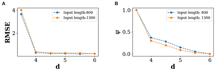
Figure 5. Predictability of extreme events. For 20 extreme events, (A) RSME against threshold d for different length of input data, (B) average phase against threshold d for different length of input data. Here, for both cases the average of 400 realizations are presented. Instantaneous phase ϕ_i(t) of ith signal is estimated using the Hilbert transform [67].

Next we introduce another measure ψ based on the instantaneous phases of the time signal inputs,

where ϕ_i(t) is the instantaneous phase of the i-th signal of the passive variable v at time t, n is the total number of segments and T is the segment length. Here, ϕ_i(t) of i th signal is calculated using the Hilbert transform [67]. High value of ψ indicates less coherent structure and vice-versa. This variable ψ represents the average phase difference (on the number of segment and segment length) between all the 180 input signals of different length.

We plot values of ψ against d for the two different time lengths (800, 1, 300) in Figure 5B. A phase coherence is observed with increasing d. When the threshold is low (lower value of d), the time signals of v are dispersed (see Figure 5A). As a result, the average phase difference ψ is high. ψ gradually converges for higher values of d with the formation of a coherent bundle of the input signals. This indicates that there is a higher tendency of phase coherence between input signals for higher magnitude EEs which enhances the ability of the machine to predict their precursory structure.

Conclusion and discussion

We have proposed an Echo State Network based scheme for the prediction of the preceding shape of extreme events from a passive variable which shows no visible manifestation of extreme events, but connected to an active variable that has clear indications of rare and recurrent high amplitude events. Such a situation occurs in the real world where maintaining data records of subsidiary variable is easier, and may be useful for studies related to prediction of extreme events in another observable that is difficult to record. To test our scheme, we generated data using a synaptically (chemical) coupled model of two Hindmarsh-Rose (HR) neurons. Two types of variables are involved in the HR model, two fast variables (defined as active) that exhibit extreme events in their time evolution, and a slow variable (defined here as passive) having a slower time-scale and most importantly, showing no visible signs of extremes. The passive variable was considered as our input candidate for the machine for the purpose of predicting the preceding structure of extreme events in the active variable.

Our strategy was first to identify the extreme events in a long time series of an active variable with a choice of an appropriate threshold height and collect data from the passive variable that corresponds to each extreme in the active variable. We saved the data only prior to the arrival of extreme events barring all extremes, then a part of the collected dataset from the passive variable is used for testing a multi-input machine and another part of the data for testing/predicting the prior structure of the forthcoming extremes. Our results indicated that higher the magnitude of extreme events, the efficiency of the machine to predict its precursory structure is higher. Higher intensity events are defined only by increasing the threshold height. On further investigation, we found that for higher intensity extreme events the input signals collectively form a coherent pattern, which aided the machine to predict the prior structure with increased efficiency. Thus, coherence of the multi-input time signals is the key to a better prediction of the forthcoming extreme events by the machine. A possible quantitative explanation of the enhanced predictability is provided. For this purpose, a new coherence measure ψ is introduced to represent the average phase differences between the segmented time signals. It was observed that ψ decreases with increasing threshold height, therefore confirming our finding that the enhanced ability of the machine to predict higher amplitude extreme events is related to an increase in the phase coherence of the input signals.

Our machine learning scheme opens up an alternative strategy for predicting extreme events from passive variables in the real world. Furthermore, our findings maintains those reported by [37, 38] that higher the magnitude of extreme events, higher is the predictability skill. Finding suitable passive variables for real world systems is a challenge. Most of the time they typically belong to very high dimensional system and often can be a combination of multiple variables. For example, Moon and Ha [68] identified the relation between the onset of Indian summer monsoon with the soil moisture in the Iranian desert, our method could be used to predict the early warning or precursory signal to the forthcoming climate extreme if we can identify the slow variables properly.

Data availability statement

In this study, the data has been generated by numerical simulation. Further inquiries can be directed to the corresponding author/s.

Author contributions

AB, NM, AM, and CH: conceptualization. AB: data curation, formal analysis, software, and visualization. AB, AM, CH, SD, and NM: investigation. AB and NM: methodology. AB, AM, SD, and NM: resources. NM and JK: supervision. AB and SD: writing–original draft preparation. AB, AM, CH, SD, TK, JK, and NM: writing—review and editing. All authors contributed to the article and approved the submitted version.

Funding

This research has been funded by the Deutsche Forschungsgemeinschaft (DFG) within graduate research training group GRK 2043/1 Natural risk in a changing world (NatRiskChange) at the University of Potsdam. TK and AM have been supported by the National Science Centre, Poland, OPUS Program Project No. 2018/29/B/ST8/00457. CH was supported by the INSPIRE-Faculty Grant (code: IFA17-PH193).

Conflict of interest

The authors declare that the research was conducted in the absence of any commercial or financial relationships that could be construed as a potential conflict of interest.

The reviewer DG declared a shared affiliation with the author(s) CH to the handling editor at the time of review.

Publisher's note

All claims expressed in this article are solely those of the authors and do not necessarily represent those of their affiliated organizations, or those of the publisher, the editors and the reviewers. Any product that may be evaluated in this article, or claim that may be made by its manufacturer, is not guaranteed or endorsed by the publisher.

Supplementary material

The Supplementary Material for this article can be found online at: https://www.frontiersin.org/articles/10.3389/fams.2022.955044/full#supplementary-material

References

1. Seneviratne S, Nicholls N, Easterling D, Goodess C, Kanae S, Kossin J, et al. Changes in Climate Extremes and Their Impacts on the Natural Physical Environment. (2012).
2. McPhillips LE, Chang H, Chester MV, Depietri Y, Friedman E, Grimm NB, et al. Defining extreme events: a cross-disciplinary review. Earths Future. (2018) 6:441–55. doi: 10.1002/2017EF000686
3. Broska LH, Poganietz WR, Vögele S. Extreme events defined–A conceptual discussion applying a complex systems approach. Futures. (2020) 115:102490. doi: 10.1016/j.futures.2019.102490
4. Bunde A, Eichner JF, Havlin S, Kantelhardt JW. The effect of long-term correlations on the return periods of rare events. Phys A Stat Mech Appl. (2003) 330:1–7. doi: 10.1016/j.physa.2003.08.004
5. Jentsch V, Kantz H, Albeverio S. In: Albeverio S, Jentsch V, Kantz H, editors. Extreme Events: Magic, Mysteries, and Challenges. Berlin; Heidelberg: Springer (2006).
6. Dysthe K, Krogstad HE, Müller P. Oceanic rogue waves. Annu Rev Fluid Mech. (2008) 40:287–310. doi: 10.1146/annurev.fluid.40.111406.102203
7. Altmann EG, Hallerberg S, Kantz H. Reactions to extreme events: moving threshold model. Phys A Stat Mech Appl. (2006) 364:435–44. doi: 10.1016/j.physa.2005.08.074
8. Kharif C, Pelinovsky E, Slunyaev A. Rogue Waves in the Ocean. Springer Science & Business Media (2008).
9. Krause SM, Börries S, Bornholdt S. Econophysics of adaptive power markets: when a market does not dampen fluctuations but amplifies them. Phys Rev E. (2015) 92:012815. doi: 10.1103/PhysRevE.92.012815
10. Marwan N, Kurths J. Complex network based techniques to identify extreme events and (sudden) transitions in spatio-temporal systems. Chaos Interdiscipl J Nonlinear Sci. (2015) 25:097609. doi: 10.1063/1.4916924
11. Ray A, Rakshit S, Basak GK, Dana SK, Ghosh D. Understanding the origin of extreme events in El Niño southern oscillation. Phys Rev E. (2020) 101:062210. doi: 10.1103/PhysRevE.101.062210
13. Sornette D. Predictability of catastrophic events: material rupture, earthquakes, turbulence, financial crashes, and human birth. Proc Natl Acad Sci USA. (2002) 99(Suppl. 1):2522–9. doi: 10.1073/pnas.022581999
14. Chowdhury SN, Ray A, Dana SK, Ghosh D. Extreme events in dynamical systems and random walkers: a review. Phys Rep. (2022) 966:1–52. doi: 10.1016/j.physrep.2022.04.001
15. Mishra A, Leo Kingston S, Hens C, Kapitaniak T, Feudel U, Dana SK. Routes to extreme events in dynamical systems: dynamical and statistical characteristics. Chaos Interdiscipl J Nonlinear Sci. (2020) 30:063114. doi: 10.1063/1.5144143
16. Farazmand M, Sapsis TP. Extreme events: mechanisms and prediction. Appl Mech Rev. (2019) 71:050801. doi: 10.1115/1.4042065
17. Chowdhury SN, Majhi S, Ozer M, Ghosh D, Perc M. Synchronization to extreme events in moving agents. N J Phys. (2019) 21:073048. doi: 10.1088/1367-2630/ab2a1f
18. Chowdhury SN, Majhi S, Ghosh D. Distance dependent competitive interactions in a frustrated network of mobile agents. IEEE Trans Netw Sci Eng. (2020) 7:3159–70. doi: 10.1109/TNSE.2020.3017495
19. Nag Chowdhury S, Kundu S, Duh M, Perc M, Ghosh D. Cooperation on interdependent networks by means of migration and stochastic imitation. Entropy. (2020) 22:485. doi: 10.3390/e22040485
20. Fan J, Meng J, Ludescher J, Chen X, Ashkenazy Y, Kurths J, et al. Statistical physics approaches to the complex Earth system. Phys Rep. (2021) 896:1–84. doi: 10.1016/j.physrep.2020.09.005
21. Boers N, Bookhagen B, Marwan N, Kurths J, Marengo J. Complex networks identify spatial patterns of extreme rainfall events of the South American Monsoon System. Geophys Res Lett. (2013) 40:4386–92. doi: 10.1002/grl.50681
22. Stolbova V, Martin P, Bookhagen B, Marwan N, Kurths J. Topology and seasonal evolution of the network of extreme precipitation over the Indian subcontinent and Sri Lanka. Nonlinear Process Geophys. (2014) 21:901–17. doi: 10.5194/npg-21-901-2014
23. Mondal S, Mishra AK. Complex networks reveal heatwave patterns and propagations over the USA. Geophys Res Lett. (2021) 48:e2020GL090411. doi: 10.1029/2020GL090411
24. Agarwal A, Guntu RK, Banerjee A, Gadhawe MA, Marwan N. A complex network approach to study the extreme precipitation patterns in a river basin. Chaos Interdiscipl J Nonlinear Sci. (2022) 32:013113. doi: 10.1063/5.0072520
25. Ghil M, Yiou P, Hallegatte S, Malamud B, Naveau P, Soloviev A, et al. Extreme events: dynamics, statistics and prediction. Nonlinear Process Geophys. (2011) 18:295–350. doi: 10.5194/npg-18-295-2011
26. Coles S. An Introduction to Statistical Modeling of Extreme Values. London: Springer-Verlag (2001).
27. Banerjee A, Goswami B, Hirata Y, Eroglu D, Merz B, Kurths J, et al. Recurrence analysis of extreme event-like data. Nonlinear Process Geophys. (2021) 28:213–29. doi: 10.5194/npg-28-213-2021
28. Karnatak R, Ansmann G, Feudel U, Lehnertz K. Route to extreme events in excitable systems. Phys Rev E. (2014) 90:022917. doi: 10.1103/PhysRevE.90.022917
29. Ray A, Mishra A, Ghosh D, Kapitaniak T, Dana SK, Hens C. Extreme events in a network of heterogeneous Josephson junctions. Phys Rev E. (2020) 101:032209. doi: 10.1103/PhysRevE.101.032209
30. Ansmann G, Karnatak R, Lehnertz K, Feudel U. Extreme events in excitable systems and mechanisms of their generation. Phys Rev E. (2013) 88:052911. doi: 10.1103/PhysRevE.88.052911
31. Amil P, Soriano MC, Masoller C. Machine learning algorithms for predicting the amplitude of chaotic laser pulses. Chaos Interdiscipl J Nonlinear Sci. (2019) 29:113111. doi: 10.1063/1.5120755
32. Qi D, Majda AJ. Using machine learning to predict extreme events in complex systems. Proc Natl Acad Sci USA. (2020) 117:52–9. doi: 10.1073/pnas.1917285117
33. Lellep M, Prexl J, Linkmann M, Eckhardt B. Using machine learning to predict extreme events in the Hénon map. Chaos Interdiscipl J Nonlinear Sci. (2020) 30:013113. doi: 10.1063/1.5121844
34. Pyragas V, Pyragas K. Using reservoir computer to predict and prevent extreme events. Phys Lett A. (2020) 384:126591. doi: 10.1016/j.physleta.2020.126591
35. Chowdhury SN, Ray A, Mishra A, Ghosh D. Extreme events in globally coupled chaotic maps. J Phys Complexity. (2021) 2:035021. doi: 10.1088/2632-072X/ac221f
36. Ray A, Chakraborty T, Ghosh D. Optimized ensemble deep learning framework for scalable forecasting of dynamics containing extreme events. Chaos Interdiscipl J Nonlinear Sci. (2021) 31:111105. doi: 10.1063/5.0074213
37. Hallerberg S, Kantz H. How does the quality of a prediction depend on the magnitude of the events under study? Nonlinear Process Geophys. (2008) 15:321–31. doi: 10.5194/npg-15-321-2008
38. Hallerberg S, Kantz H. Influence of the event magnitude on the predictability of an extreme event. Phys Rev E. (2008) 77:011108. doi: 10.1103/PhysRevE.77.011108
39. Lukoševičius M. In: Montavon G, Orr GB, Müller KR, editors. A Practical Guide to Applying Echo State Networks. Berlin; Heidelberg: Springer (2012).
40. Jaeger H, Haas H. Harnessing nonlinearity: predicting chaotic systems and saving energy in wireless communication. Science. (2004) 304:78–80. doi: 10.1126/science.1091277
41. Pathak J, Hunt B, Girvan M, Lu Z, Ott E. Model-free prediction of large spatiotemporally chaotic systems from data: a reservoir computing approach. Phys Rev Lett. (2018) 120:024102. doi: 10.1103/PhysRevLett.120.024102
42. Zimmermann RS, Parlitz U. Observing spatio-temporal dynamics of excitable media using reservoir computing. Chaos Interdiscipl J Nonlinear Sci. (2018) 28:043118. doi: 10.1063/1.5022276
43. Pathak J, Lu Z, Hunt BR, Girvan M, Ott E. Using machine learning to replicate chaotic attractors and calculate Lyapunov exponents from data. Chaos Interdiscipl J Nonlinear Sci. (2017) 27:121102. doi: 10.1063/1.5010300
44. Lin X, Yang Z, Song Y. Short-term stock price prediction based on echo state networks. Expert Syst Appl. (2009) 36(3 Pt 2):7313–7. doi: 10.1016/j.eswa.2008.09.049
45. Hinaut X, Dominey PF. Real-time parallel processing of grammatical structure in the fronto-striatal system: a recurrent network simulation study using reservoir computing. PLoS ONE. (2013) 8: e52946. doi: 10.1371/journal.pone.0052946
46. Verstraeten D, Schrauwen B, Stroobandt D, Van Campenhout J. Isolated word recognition with the Liquid State Machine: a case study. Inform Process Lett. (2005) 95:521–8. doi: 10.1016/j.ipl.2005.05.019
47. Lu Z, Hunt BR, Ott E. Attractor reconstruction by machine learning. Chaos Interdiscipl J Nonlinear Sci. (2018) 28:061104. doi: 10.1063/1.5039508
48. Mandal S, Sinha S, Shrimali MD. Machine-learning potential of a single pendulum. Phys Rev E. (2022) 105:054203. doi: 10.1103/PhysRevE.105.054203
49. Lu Z, Pathak J, Hunt B, Girvan M, Brockett R, Ott E. Reservoir observers: model-free inference of unmeasured variables in chaotic systems. Chaos Interdiscipl J Nonlinear Sci. (2017) 27:041102. doi: 10.1063/1.4979665
50. Thiede LA, Parlitz U. Gradient based hyperparameter optimization in echo state networks. Neural Netw. (2019) 115:23–9. doi: 10.1016/j.neunet.2019.02.001
51. Weng T, Yang H, Gu C, Zhang J, Small M. Synchronization of chaotic systems and their machine-learning models. Phys Rev E. (2019) 99:042203. doi: 10.1103/PhysRevE.99.042203
52. Lymburn T, Walker DM, Small M, Jungling T. The reservoir's perspective on generalized synchronization. Chaos Interdiscipl J Nonlinear Sci. (2019) 29:093133. doi: 10.1063/1.5120733
53. Chen X, Weng T, Yang H, Gu C, Zhang J, Small M. Mapping topological characteristics of dynamical systems into neural networks: a reservoir computing approach. Phys Rev E. (2020) 102:033314. doi: 10.1103/PhysRevE.102.033314
54. Panday A, Lee WS, Dutta S, Jalan S. Machine learning assisted network classification from symbolic time-series. Chaos Interdiscipl J Nonlinear Sci. (2021) 31:031106. doi: 10.1063/5.0046406
55. Fan H, Kong LW, Lai YC, Wang X. Anticipating synchronization with machine learning. Phys Rev Res. (2021) 3:023237. doi: 10.1103/PhysRevResearch.3.023237
56. Xiao R, Kong LW, Sun ZK, Lai YC. Predicting amplitude death with machine learning. Phys Rev E. (2021) 104:014205. doi: 10.1103/PhysRevE.104.014205
57. Mandal S, Shrimali MD. Achieving criticality for reservoir computing using environment-induced explosive death. Chaos. (2021) 31:031101. doi: 10.1063/5.0038881
58. Saha S, Mishra A, Ghosh S, Dana SK, Hens C. Predicting bursting in a complete graph of mixed population through reservoir computing. Phys Rev Res. (2020) 2:033338. doi: 10.1103/PhysRevResearch.2.033338
59. Ghosh S, Senapati A, Mishra A, Chattopadhyay J, Dana SK, Hens C, et al. Reservoir computing on epidemic spreading: a case study on COVID-19 cases. Phys Rev E. (2021) 104:014308. doi: 10.1103/PhysRevE.104.014308
60. Roy M, Senapati A, Poria S, Mishra A, Hens C. Role of assortativity in predicting burst synchronization using echo state network. Phys Rev E. (2022) 105:064205. doi: 10.1103/PhysRevE.105.064205
61. LeCun Y, Bengio Y, Hinton G. Deep learning. Nature. (2015) 521:436–444. doi: 10.1038/nature14539
62. Zamora-Munt J, Garbin B, Barland S, Giudici M, Leite JRR, Masoller C, et al. Rogue waves in optically injected lasers: origin, predictability, and suppression. Phys Rev A. (2013) 87:035802. doi: 10.1103/PhysRevA.87.035802
63. Bonatto C, Endler A. Extreme and superextreme events in a loss-modulated CO 2 laser: nonlinear resonance route and precursors. Phys Rev E. (2017) 96:012216. doi: 10.1103/PhysRevE.96.012216
64. Hindmarsh J, Rose R. A model of the nerve impulse using two first-order differential equations. Nature. (1982) 296:162–4. doi: 10.1038/296162a0
65. Mishra A, Saha S, Vigneshwaran M, Pal P, Kapitaniak T, Dana SK. Dragon-king-like extreme events in coupled bursting neurons. Phys Rev E. (2018) 97:062311. doi: 10.1103/PhysRevE.97.062311
66. Bonatto C, Feyereisen M, Barland S, Giudici M, Masoller C, Leite JRR, et al. Deterministic optical rogue waves. Phys Rev Lett. (2011) 107:053901. doi: 10.1103/PhysRevLett.107.053901
67. Rosenblum MG, Pikovsky AS, Kurths J. Phase synchronization of chaotic oscillators. Phys Rev Lett. (1996) 76:1804. doi: 10.1103/PhysRevLett.76.1804
Keywords: extreme events, coupled neuron model, active and passive variable, precursory structure, echo state network, phase coherence
Citation: Banerjee A, Mishra A, Dana SK, Hens C, Kapitaniak T, Kurths J and Marwan N (2022) Predicting the data structure prior to extreme events from passive observables using echo state network. Front. Appl. Math. Stat. 8:955044. doi: 10.3389/fams.2022.955044
Received: 28 May 2022; Accepted: 30 September 2022;
Published: 20 October 2022.
Edited by:
Ulrich Parlitz, Max Planck Society, GermanyReviewed by:
Dibakar Ghosh, Indian Statistical Institute, IndiaNahal Sharafi, Hamburg University of Applied Sciences, Germany
Copyright © 2022 Banerjee, Mishra, Dana, Hens, Kapitaniak, Kurths and Marwan. This is an open-access article distributed under the terms of the Creative Commons Attribution License (CC BY). The use, distribution or reproduction in other forums is permitted, provided the original author(s) and the copyright owner(s) are credited and that the original publication in this journal is cited, in accordance with accepted academic practice. No use, distribution or reproduction is permitted which does not comply with these terms.
*Correspondence: Abhirup Banerjee, banerjee@pik-potsdam.de