
A systematic comparison of transfer learning models for COVID-19 prediction
Abstract
The pandemic COVID-19 is already in its third year and there is no sign of ebbing. The world continues to be in a never-ending cycle of disease outbreaks. Since the introduction of Omicron-the most mutated and transmissible of the five variants of COVID-19 – fear and instability have grown. Many papers have been written on this topic, as early detection of COVID-19 infection is crucial. Most studies have used X-rays and CT images as these are highly sensitive to detect early lung changes. However, for privacy reasons, large databases of these images are not publicly available, making it difficult to obtain very accurate AI Deep Learning models. To address this shortcoming, transfer learning (pre-trained) models are used. The current study aims to provide a thorough comparison of known AI Deep Transfer Learning models for classifying lung radiographs into COVID-19, non COVID pneumonia and normal (healthy). The VGG-19, Inception-ResNet, EfficientNet-B0, ResNet-50, Xception and Inception models were trained and tested on 3568 radiographs. The performance of the models was evaluated using accuracy, sensitivity, precision and F1 score. High detection accuracy scores of 98% and 97% were found for the VGG-19 and Inception-ResNet models, respectively.
1.Introduction
The outbreak of COVID-19 is still ongoing. By the last week of January 2022, the new coronavirus has wreaked havoc in nearly 200 countries, killing an estimated 5.3 million people [1]. The fear and chaos have intensified since the emergence of Omicron, the most mutated and transmissible version of the COVID-19 [2]. More than 100 countries have adopted lockdowns and closures and announced restrictions on gatherings by the last week of December 2021. The behaviour of the new Omicron variant in terms of its widespread distribution and the expression of symptoms has astonished the research community. The most common symptoms in COVID-19 patients are fever, cough and fatigue [3]. Identifying COVID-19 can be difficult, especially during flu season, as these symptoms can also occur in patients with pneumonia. WHO has approved reverse transcription-polymerase chain reaction (RT-PCR) as a test method for COVID-19, which analyses RNA sequences to determine the presence of coronavirus [1]. False-negative cases and a shortage of test kits and screening workstations are causing bottlenecks, especially in pandemic hotspots in developing countries. Since COVID-19-induced pneumonia has a higher mortality rate in some ethnic groups, early identification of COVID-19 is critical. The unpredictability of the incubation period, which can range from 1 to 14 days between infection with the virus and the onset of symptoms, makes early detection even more difficult. These difficulties highlight the need to develop new COVID-19 detection methods [4].
Early studies discovered abnormalities in chest X-rays of COVID-19 infected people that could help diagnose the disease. COVID-19 has been associated with an increase in lung density and emphysema. Chronic obstructive pulmonary disease can be life-threatening as a result of this [5]. Horizontal white lines, bands or reticular changes and a ground-glass opacity characterise a COVID-19 radiograph of the lungs [6]. As a result, disease classification based on chest radiographs/(CT) has become a viable option to aid medical diagnosis, especially in the pandemic area. Chest radiography has a cost advantage and higher sensitivity than CT imaging [7]. Given the shortage of test kits and screening stations, the availability of X-ray equipment is an attractive option for COVID-19 detection. In contrast, manual detection of COVID-19 on chest radiographs, which include both COVID-19 and pneumonia cases, is time-consuming and requires the presence of experienced medical personnel [8]. It is also prone to human error. Therefore, artificial intelligence systems based on deep learning algorithms that learn from X-ray images and predict the presence of COVID-19 have the potential to improve the current diagnostic process.
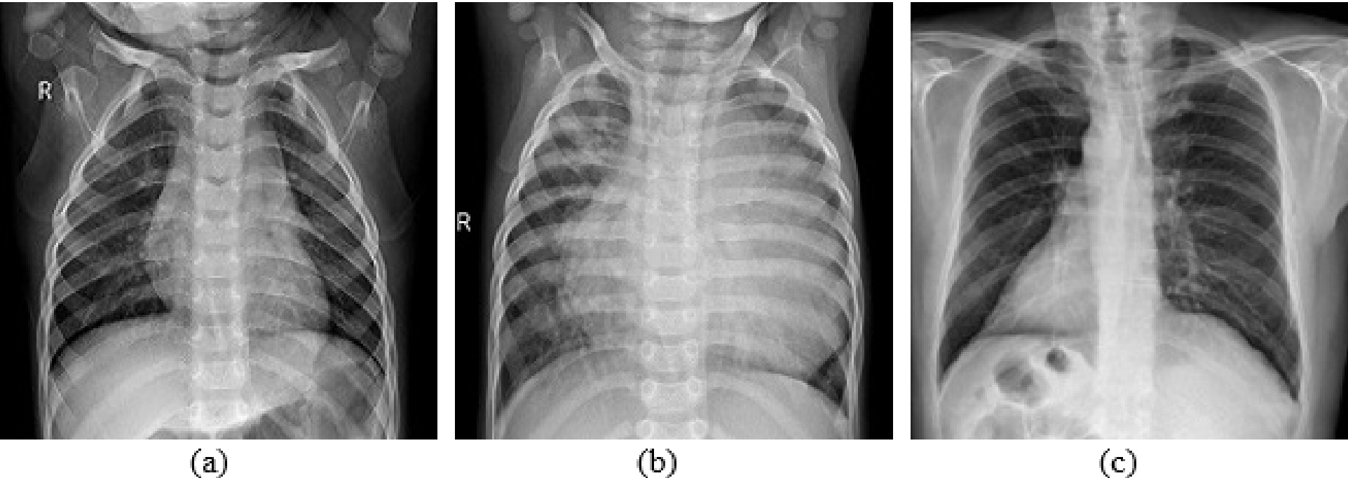
Figure 1.
X-ray image types a) healthy b) non-COVID pneumonia c) COVID-19.
According to recent studies, Deep Learning algorithms have been successfully deployed in a number of clinical applications, including breast cancer detection, brain disease classification, diabetic retinopathy, fundus image segmentation, cardiac arrhythmia detection, pneumonia, lung segmentation and skin cancer classification [9]. Deep learning is a type of machine learning that focuses on learning from enormous amounts of information and enables the creation of a powerful end-to-end model without the use of feature extraction. Most traditional learning systems start from scratch for each classification task, creating and training new baselines and classifiers. Convolutional networks often perform better on large datasets, while smaller datasets degrade their performance. Training a deep network from scratch usually requires large datasets, but access to these data is not always possible, such as with medical images – this is where transfer learning comes in [10]. Faster training times, improved neural network performance (in most cases) and the need for less data are just some of the benefits of transfer learning [11]. A model trained for one task (when a large dataset is available) is fine-tuned in transfer learning for a second task (when only a small dataset is available). In addition to supporting model reuse, learned features and complete models for classification, regression and clustering tasks can be reused in a related task with transfer learning [12]. In this study, we critically evaluate the performance of six commonly employed transfer learning models for COVID-19 recognition. 3568 X-ray images from the dataset of Cohen et al. [13] and Wang et al. [14] were used to train and test the VGG-19, Inception-ResNet, EfficientNet-B0, ResNet-50, Xception and Inception models. All models were adapted to the three-class classification of lung radiographs into COVID-19, non-COVID pneumonia and normal (healthy). The accuracy, sensitivity, precision and F1 score of all models were investigated. The VGG-19 and Inception-ResNet models achieved high recognition accuracy of 98% and 97%, respectively.
1.1Organization of the paper
The rest of the paper is structured as follows. The following section gives a brief overview of related work in the literature. The rationale for the transfer learning models employed in this comparative study and the implementation details are presented in Section 3. The findings of the tests as well as the database and experimental setup are explained in Section 4. Section 5 of the paper concludes with a conclusion.
2.Related work
Using deep learning technology, a number of research studies have been conducted to investigate automated radiographs of the lungs to distinguish patients with pneumonia and COVID-19. Many authors investigated the performance of transfer learning approaches for COVID-19 screening [15, 16, 17, 18, 19, 12, 20, 21, 22, 23, 24, 25, 26, 27, 28, 29]. Narin et al. [15], for example, created three CNN-based models using the current transfer learning architecture and found that the ResNet model had the best classification accuracy. Only 50 COVID-19 patients and 50 healthy individuals participated in the study. By combining three different models that were fine-tuned in three datasets, they developed a multi-channel ensemble transfer learning technique based on ResNet-18 that enabled the model to extract more important features for each class and thus better recognise COVID-19 features from radiographs.
Chouhan et al. [16] employed an ensemble model to classify pneumonia and normal radiographs. They claimed to have achieved the best performance by using an ensemble approach combining five different pre-trained models. Previous studies have shown that Deep Learning algorithms can improve computer vision tasks such as image classification. Using state-of-the-art artificial intelligence approaches, most of the methods described achieved classification accuracy of more than 90%. The experiments of the different methods were on a COVID-19 X-ray image database of limited size (25–864), so their efficiency and performance cannot be generalised to a much larger dataset. Despite these limitations, the current study used a larger dataset (3568 lung X-ray samples) to address the challenge of generalisation with small datasets. In this work, we investigate the performance of pre-trained models for accurate identification of COVID-19. To find the best algorithms, each algorithm is fine-tuned to increase detection accuracy.
3.Materials and methods
Deep learning algorithms are becoming more popular as the amount of data and processing capacity increases. Artificial neural networks (ANNs) are the most commonly used deep learning algorithms, with convolutional neural networks (CNNs) being the most popular (ANNs). CNNs are widely used in computer vision, image analysis and pattern recognition. The LeNet-5, a seven-layer CNN, is the cornerstone of the current CNN design. The fundamentals of the proposed model are explored in [9]. These methods have proven successful in clinical diagnosis of a wide range of diseases. Deep Learning methods require numerous epochs of training and validation to achieve optimal performance. Deep Learning requires an enormous amount of data to eliminate the fitting problems and increase efficiency. It is difficult to obtain large datasets for medical images of severe diseases. Therefore, better classification strategies are essential to generalise the performance of the systems. Transfer learning significantly increases the learning efficiency of the model in these cases [30]. Transfer learning is a form of deep learning in which a model created for one task is used to create another model [31]. So it allows better output for Deep Learning algorithms in the desired research domain. Suppose we have a model trained with the ImageNet database. With the help of transfer learning, we can reuse the same model (the knowledge acquired while training the model can be used) for another database, for example, an X-ray image database. Transfer learning greatly improves and facilitates the training of deep neural networks. The different steps in transfer learning are:
• Model selection: A pre-trained source model is selected from the available models.
• Model reuse: The pre-trained model can then be used as the basis for developing a model for the second job of interest. Depending on the modelling process, this may mean that the whole model or only parts of it are used.
• Model tuning: Optionally, the model needs to be modified or optimised depending on the available input-output data for the task of interest.
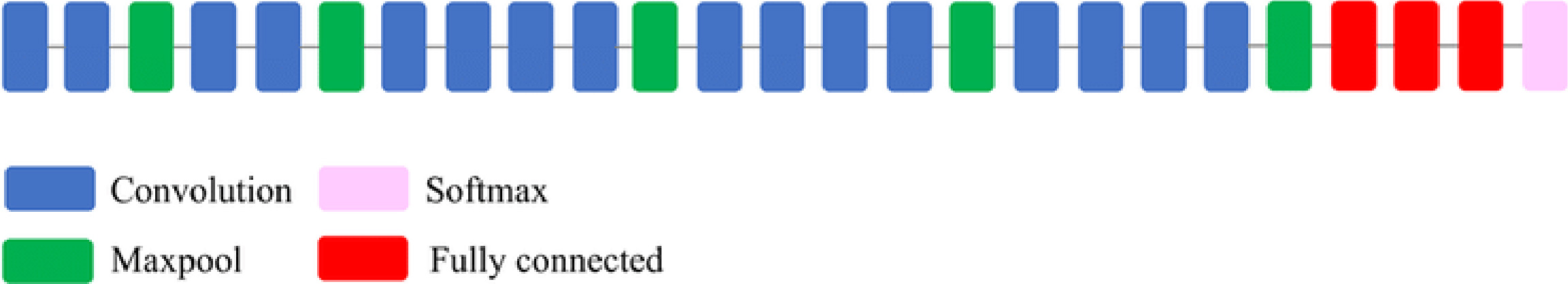
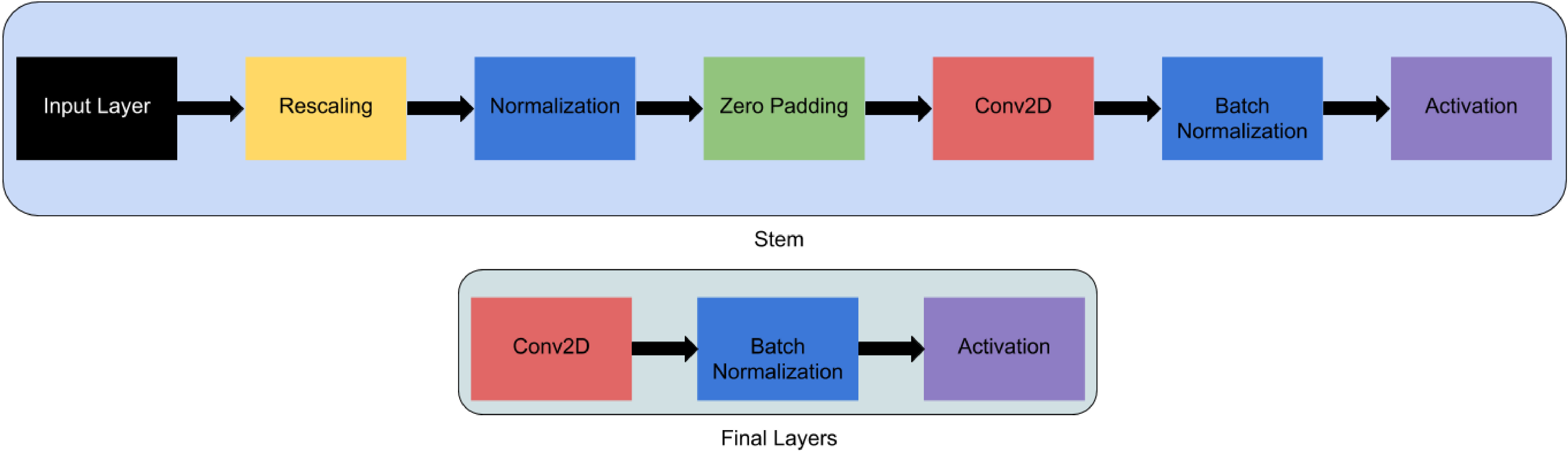
Figure 2.
Schematic diagram of VGG-19 model.
In transfer learning, the fully connected layers of a pre-trained CNN architecture learned with a large dataset (such as ImageNet) are removed from the network. For the new dataset, the remaining CNN is used as a fixed feature extractor. The gradient descent approach, also known as a backpropagation algorithm, is used to fine-tune the parameters (weights) of a pre-trained model for the current dataset that has already been trained for an application. Fine-tuning can be done for all layers as it improves generalisation if enough examples are available. For overfitting reasons, the earlier layers of the network can be fixed and fine-tuning is only done for the higher layers, especially for the fully connected layers. The reason for this is that the features trained in the early layers of the network are domain-independent and are more general features. In contrast, the features that are learned in the later part of the deep neural network are mostly domain-dependent. Thus, during transfer learning, the parameters of the earlier layers are fixed and the later layers are fine-tuned. Compared to training from scratch with the target dataset, transfer learning and fine-tuning generally yield better results. Even features transferred from other tasks often perform better than those with arbitrary initial weights. Consequently, transfer learning reduces training time, increases performance in most scenarios, and eliminates the need for a huge dataset [31].
The current work performs a systematic comparison of world-class pre-trained models to develop a better deep-learning solution for rapid detection of COVID-19 and non-COVID pneumonia from lung radiographs. This work demonstrates the effectiveness of six highly accurate and efficient AI deep transfer learning models (VGG-19, Inception-ResNet, EfficientNet-B0, ResNet-50, Xception and Inception models) for predicting COVID-19 and non-COVID pneumonia from lung X-ray images. The models were trained and tested using 3600 radiographs from the Kaggle dataset. The accuracy, sensitivity, precision and F1 score of the model were tested. The VGG-19 and Inception-ResNet models showed a recognition accuracy of 98% and 97% respectively, for classifying X-ray images into COVID-19, non-COVID pneumonia and normal.
The following sections give a brief overview of the widely used transfer learning models considered in this work.
3.1VGG net
In 2014, the ImageNet Large Scale Visual Recognition Challenge (ILSVRC) was a public challenge that asked participants to create the best neural network they could use to classify a database of a large number of images. The training set included 1.2 million images, each of which was manually labelled with one of the 1000 objects that the network was to recognise. There were several sub-competitions, each with its own winner. VGG-16, a network, was the winner of one of the classification tasks. The VGG network was developed by the “Visual Geometry Group”, hence the model is abbreviated as VGG. In a conventional CNN, the convolution layer, the nonlinearity layer and the pooling layer are stacked one after the other. The number of these triplets stacked in a network is determined by the depth of the network. VGG designs are based on a simple idea. We need to stack the convolutional layers as the filter sizes get larger. Layer 2 must have at least 16 filters if layer 1 has 16 filters. VGG-16 and VGG-19 are the widely used variants of the VGG network. The number 16 or 19 alludes to the 16 or 19 computational layers of the CNN network (there are also some auxiliary layers for pooling and padding). All layers have adjustable parameters.
Table 1
VGG-19 model summary
| Layer (type) | Output shape | Parameters |
| Input (InputLayer) | (None, 128, 128, 3) | 0 |
| Block1 conv1 (Conv2D) | (None, 128, 128, 64) | 1792 |
| Block1 conv2 (Conv2D) | (None, 128, 128, 64) | 36928 |
| Block1 pool (MaxPooling2D) | (None, 64, 64, 64) | 0 |
| Block2 conv1 (Conv2D) | (None, 64, 64, 128) | 73856 |
| Block2 conv2 (Conv2D) | (None, 64, 64, 128) | 147584 |
| Block2 pool (MaxPooling2D) | (None, 32, 32, 128) | 0 |
| Block3 conv1 (Conv2D) | (None, 32, 32, 256) | 295168 |
| Block3 conv2 (Conv2D) | (None, 32, 32, 256) | 590080 |
| Block3 conv3 (Conv2D) | (None, 32, 32, 256) | 590080 |
| Block3 conv4 (Conv2D) | (None, 32, 32, 256) | 590080 |
| Block3 pool (MaxPooling2D) | (None, 16, 16, 256) | 0 |
| Block4 conv1 (Conv2D) | (None, 16, 16, 512) | 1180160 |
| Block4 conv2 (Conv2D) | (None, 16, 16, 512) | 2359808 |
| Block4 conv3 (Conv2D) | (None, 16, 16, 512) | 2359808 |
| Block4 conv4 (Conv2D) | (None, 16, 16, 512) | 2359808 |
| Block4 pool (MaxPooling2D) | (None, 8, 8, 512) | 0 |
| Block5 conv1 (Conv2D) | (None, 8, 8, 512) | 2359808 |
| Block5 conv2 (Conv2D) | (None, 8, 8, 512) | 2359808 |
| Block5 conv3 (Conv2D) | (None, 8, 8, 512) | 2359808 |
| Block5 conv4 (Conv2D) | (None, 8, 8, 512) | 2359808 |
| Block5 pool (MaxPooling2D) | (None, 4, 4, 512) | 0 |
| Flatten (Flatten) | (None, 8192) | 0 |
| Dense (Dense) | (None, 3) | 24579 |
| Total params: 20,048,963 | ||
| Trainable params: 24,579 | ||
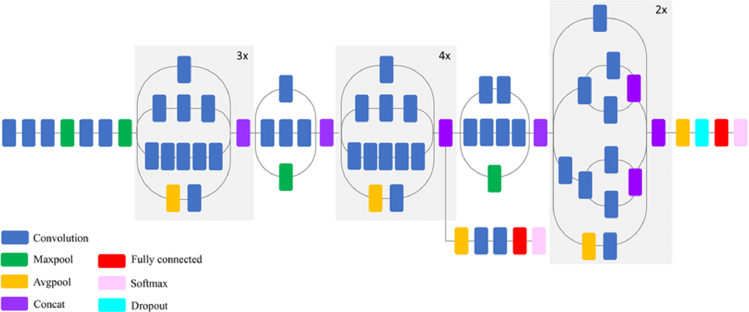
Figure 3.
Block diagram of VGG-19 model.
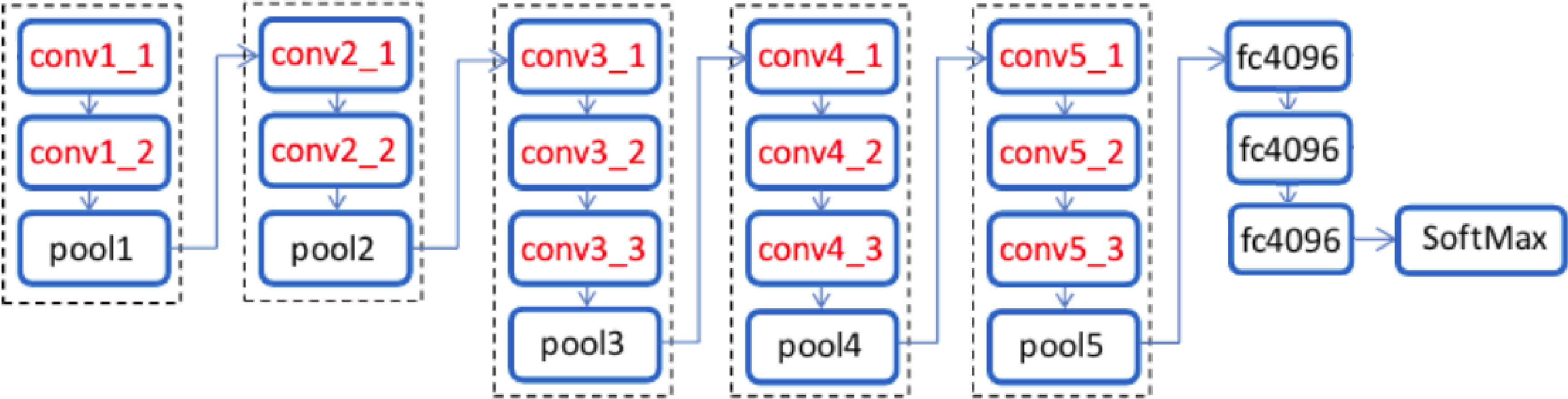
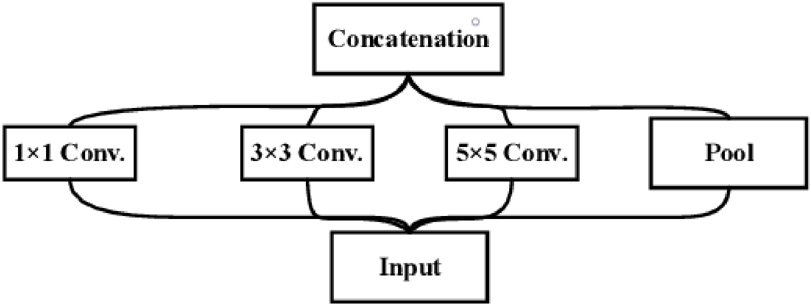
Figure 4.
Block diagram of inception model.
VGG-19: VGG-19 is an improvised version of its predecessor VGG-16. The main difference between VGG-16 and VGG-19 is the number of layers both have. VGG-19 contains three additional convolutional layers than VGG-16. VGG-19 has 16 convolutional layers, three completely connected layers, five MaxPool layers and one SoftMax layer, in addition to three fully connected layers. The input was a fixed-size RGB image of size 224
Figure 5.
Schematic diagram of Inception model.
3.2Inception net
The Inception network (GoogleLeNet) is a major milestone in CNN classifiers. The architecture has reached the state of the art in classification with the ImageNet dataset. The inception modules are repeated in the deep neural inception network to achieve the required depth. The inception module shown in Fig. 4 consists of three convolutional layers and a max-pooling layer. Each convolution layer has filtres of different sizes. Finally, all filter maps are concatenated by the filter concatenation module. The model learns from parallel filters of different sizes and scales. Usually, each image in a training set has a large variation in the location of the information. Therefore, it is very difficult to choose the right filter size. If the location in an image is small, small filtres are sufficient. When the location is large, large philtres are required to effectively capture the information content. Therefore, filtres of different sizes are used in the Inception network to effectively capture all types of information content. The schematic diagram of the Inception module is shown in Fig. 5. The goal of the Inception module is to act as a “multi-level feature extractor” by computing 1
Inception-v3: Inception-v3 is an enhanced version of GoogleLeNet that has proven to be very powerful classifier in a number of biomedical applications. It uses a transfer learning method and has 24 million parameters distributed across its 48 layers. Instead of using many convolutional filters of different sizes, a single 7
• The larger convolutions of the model were factorised into smaller convolutions, resulting in a relative gain of 28%.
• The
• The advantage of an auxiliary classifier is that it acts as a regulariser, improving the convergence of the deep neural network and combating the vanishing gradient problem.
• The activation dimension of the network filters (filter banks) is increased in the inception-v3 model to efficiently reduce the grid size.
Figure 6.
Schematic diagram of ResNet-50 model.
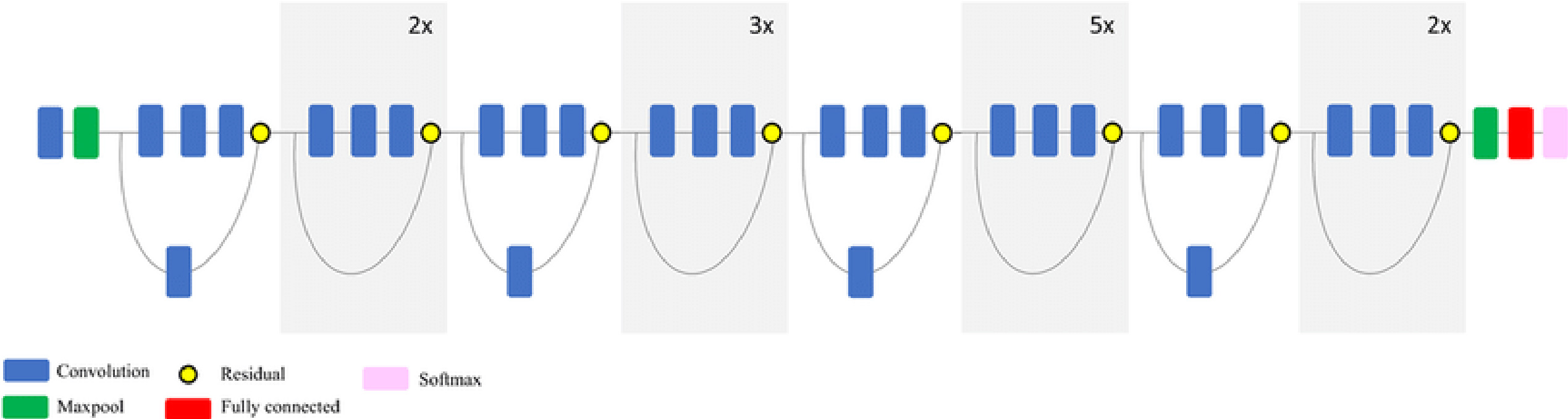
Figure 7.
Block diagram of ResNet-50 model.
3.3ResNet
ResNet stands for Residual Network. As the size of the network increases, the problem of vanishing gradients arises. As the layers get deeper, the gradient may become too small for effective training. In such a case, the gradient of the loss function approaches zero, which makes training the network very difficult. Backpropagation is used to find the gradients of the neural network. Backpropagation finds the derivatives of the network by moving from the last layer to the first layer. The derivatives of the initial layers are determined using the chain rule by multiplying the derivatives of each layer in the entire network from the last layer to the first layer. For example, if ‘
Figure 8.
Schematic diagram of Inception ResNet model.
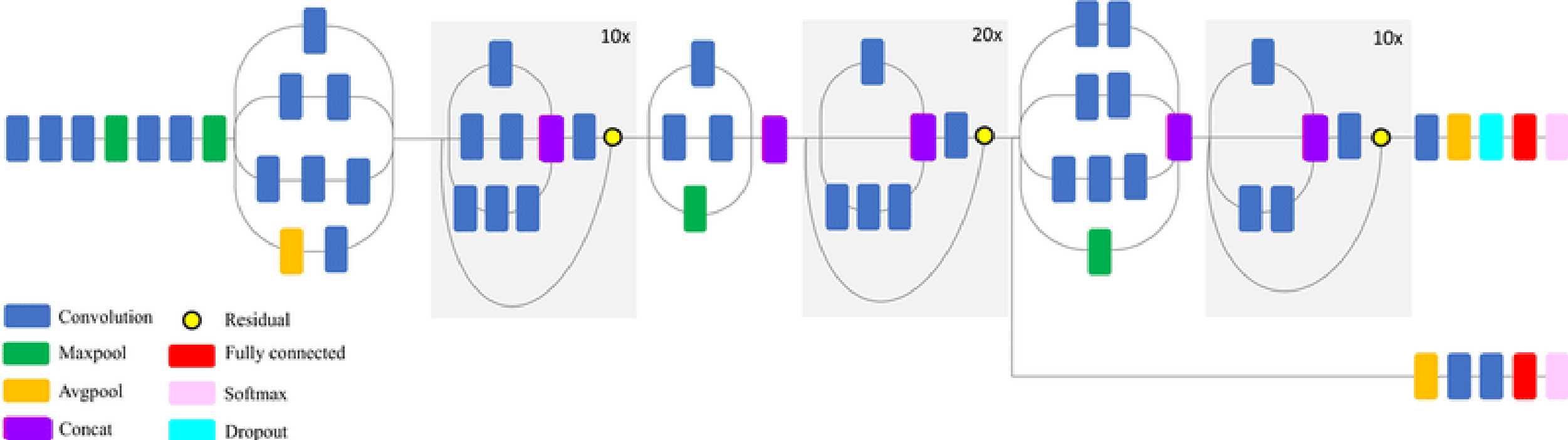
Figure 9.
Block diagram of EfficientNet-B0 model.
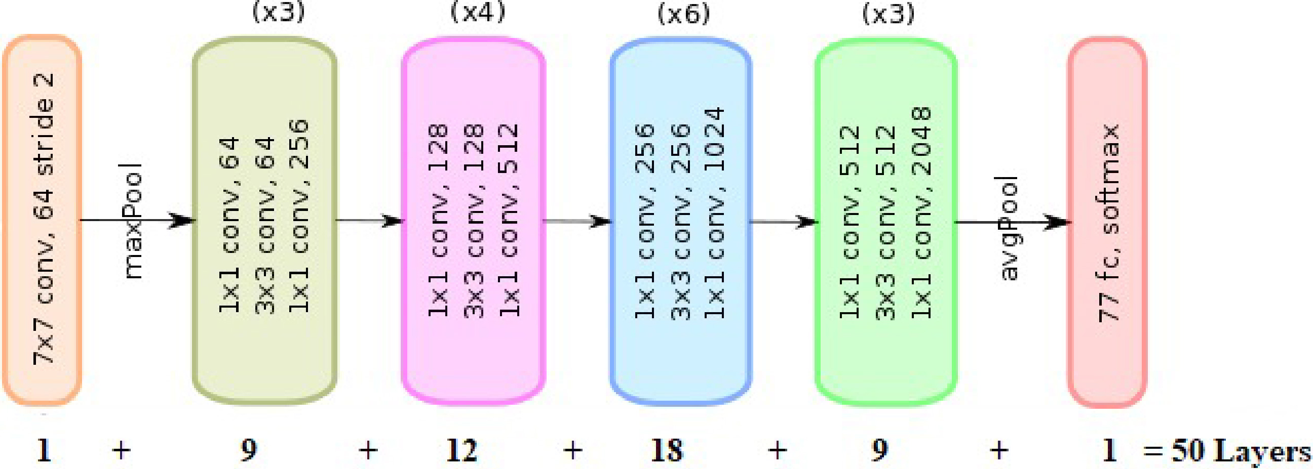
ResNet-50: ResNet comes in a variety of variants, each with a different number of layers but the same basic principle. The most popular model is ResNet-50, which has 48 convolutional layers and 2 pooling layers (a max pool and an average pool) with 3.8
The ResNet-50 model is shown schematically in Fig. 7. Each of the five phases of the ResNet-50 model has its own convolutional block and identity block. There are three convolutional layers in each convolutional block and three convolutional layers in each identity block. The ResNet-50 has approximately 23 million trainable parameters.
3.4Inception-ResNet
ResNet and Inception have made the most significant breakthroughs in image recognition performance in recent years, delivering outstanding results at low computational cost. The Inception-ResNet architecture combines Inception with ResNet connections. The network takes a 299
3.5EfficientNet
EfficientNets are lightweight models developed by Google for image classification tasks. The EfficientNet scaling approach uses a set of preset scaling coefficients to proportionally scale the resolution (number of pixels), depth (layers) and width (feature maps) of the network. The compound scaling method is justified by the assumption that higher resolution of the input image contributes to more complex features and finer patterns. The network captures (learns) more information (features) and naturally the network’s learning ability is higher and the network will be more accurate. When more information is available, deeper networks are required to process the information effectively. This facilitates the need for depth scaling of the network. Width scaling increases the number of channels or feature maps. To effectively capture more fine-grained information from a high-resolution image, we obviously need more feature maps. Width scaling widens the network.
Figure 10.
Schematic diagram of Xception model.
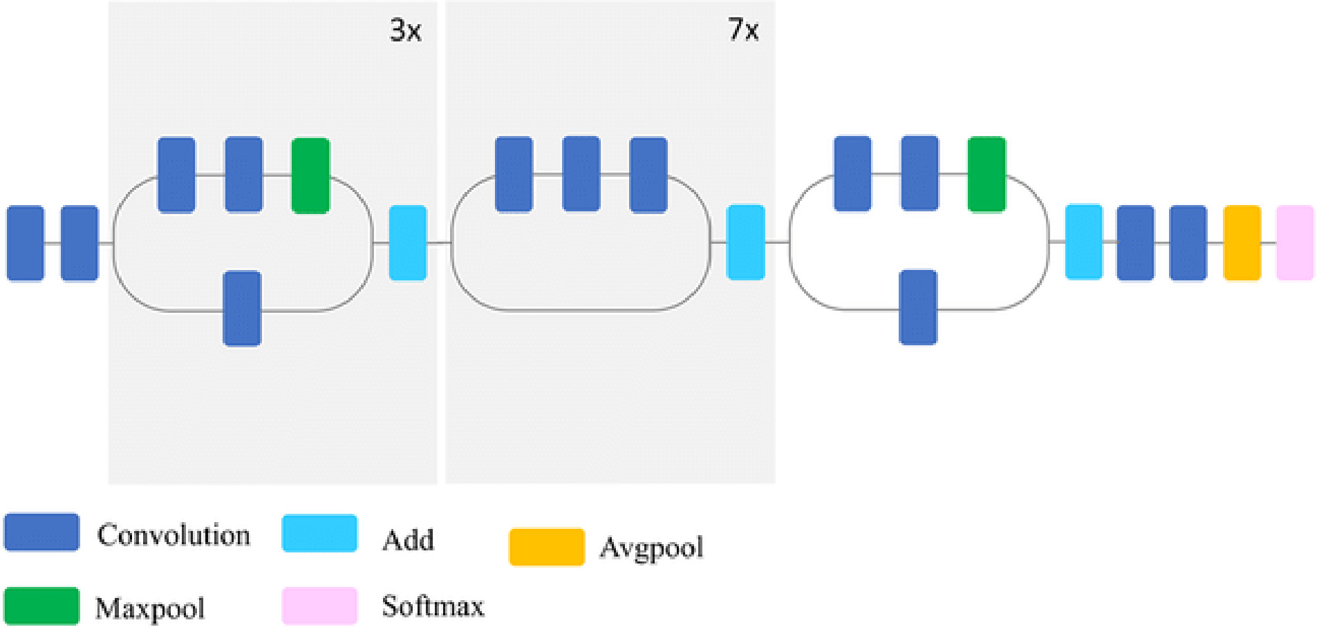
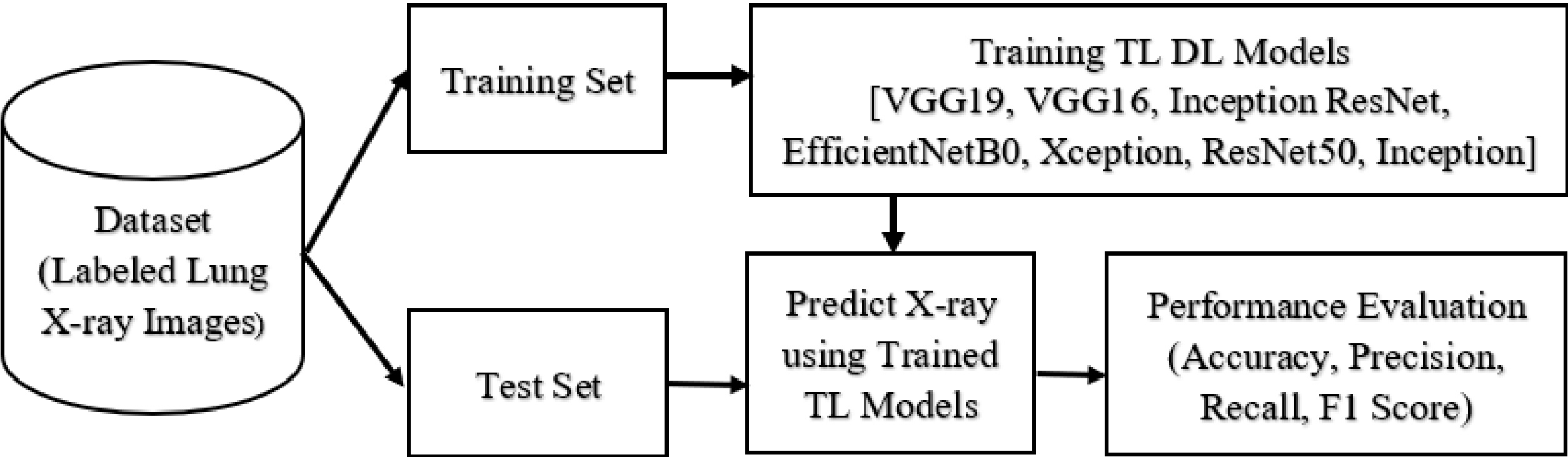
Figure 11.
Block diagram of the proposed study.
EfficientNets is a network that ranges from B0 to B7. The EfficientNet-B0 architecture is a basic model for the compound scaling. The base model is developed with NAS ( Neural Architecture Search). The base models are scaled to produce other models from B1 to B6. The compound scaling results from the following equation,
(1)
(2)
where ‘
3.6Xception
The Xception model is a refinement of the Inception v3 architecture that uses modified depthwise separable convolutions instead of the typical Inception modules (depthwise convolution followed by a pointwise convolution). The channelwise
3.7Pseudo code of the proposed model
The pseudo-code of the proposed transfer learning approach is explained in more detail below. The block diagram is shown in Fig. 11.
• begin
– Split the labelled chest X-ray dataset into a test and a training dataset;
– Select a known transfer learning model;
– Modify the first and last layers of the AI model.
– Train and validate the transfer-learned AI model and fine-tune the model;
– Predict the test data with the trained model,
– Evaluated and compared the performance of the model.
• end
4.Results and discussion
4.1Experimental set-up
The proposed study evaluates the performance of widely used transfer learning models for classifying lung radiographs into COVID-19, non COVID pneumonia and normal. Python 3.6.9 was used to develop all models. This study uses an open-source software library called Tensor-Flow, which is widely used in machine learning applications. Keras, a high-level neural network library built on top of Tensor-Flow, was used in this study. The development environment for this project was Google Colab.
For this experimental study, X-rays of the lungs were used, which are regularly updated from a variety of free sources. A total of 3568 X-ray images were considered for the experiment. Radiographs from Cohen et al. [13] and Wang et al. [14] were included in the experimental dataset. The radiologist classified these radiographs as COVID-19 (1168), non-COVID pneumonia (1200) and normal (1200). All models were trained and tested on the same dataset. Figure 1 shows an example of radiographs used in this study. 80% (2854) of the total 3568 lung radiographs selected for the study were used for training and 20% (714) for testing the transfer learning model. Before training, the labelled radiographs were preprocessed and all radiographs of different sizes were scaled to a uniform size of 128
Here, the model training is divided into a training phase and a validation phase. Therefore, the total training samples were divided into two groups: 80% for model training (2284) and 20% for internal validation (570). During the model development phase, a validation test was performed in conjunction with the training procedure to ensure that the training was correct. The models were trained in batches with a batch size of 50. In total, the networks were trained for 25 epochs. The same experimental setup was used to develop and test all transfer learning models. This enabled an efficient comparison of the six models. By optimising the algorithm during training, neural networks can be trained faster and loss functions facilitate the optimisation of the CNN parameters. For all transfer learning models, we used the vms prop optimiser (gradient descent technique) and the categorical cross entropy loss function.
4.2Performance evaluation metrics
The performance of all models for multiclass classification was evaluated using accuracy, sensitivity, precision and F1 score [31]. Since we considered the symmetric dataset, accuracy is an important metric that indicates the performance of the proposed models. The proposed model is judged by how well it correctly predicts disease based on the test radiographs. Accuracy can be calculated using the confusion matrix. The confusion matrix shows the actual and predicted classes of the classification system. The matrix shows the extent to which the classifier was confused or mistaken about some of the data. The elements of the confusion matrix in each column represent instances of the predicted class, while the elements of the confusion matrix in each row represent instances of the actual class. The diagonal elements reflect the number of correct predictions, while the non-diagonal elements represent the number of incorrect predictions. The accuracy of the classification is calculated as the number of correct predictions divided by the total number of predictions [32, 33]. Here, the accuracy is determined using the confusion matrix as follows,
(3)
Where,
• True positive (TP): The prediction is +ve and the actual (ground truth) is also +ve, i.e. the person is ill, emergency treatment is required.
• True negative (TN): The prediction is -ve and the reality is -ve, i.e. the person is not ill, treatment is not required.
• False positive (FP): The prediction is +ve and the actual is -ve, false alarm, bad, i.e. the person is not ill; but the test confirms that he is ill; this would be a gross error.
• False negative (FN): The prediction is -ve and the reality is +ve, which is the worst. i.e. the person is ill, but the test shows that he is not ill, which is even worse.
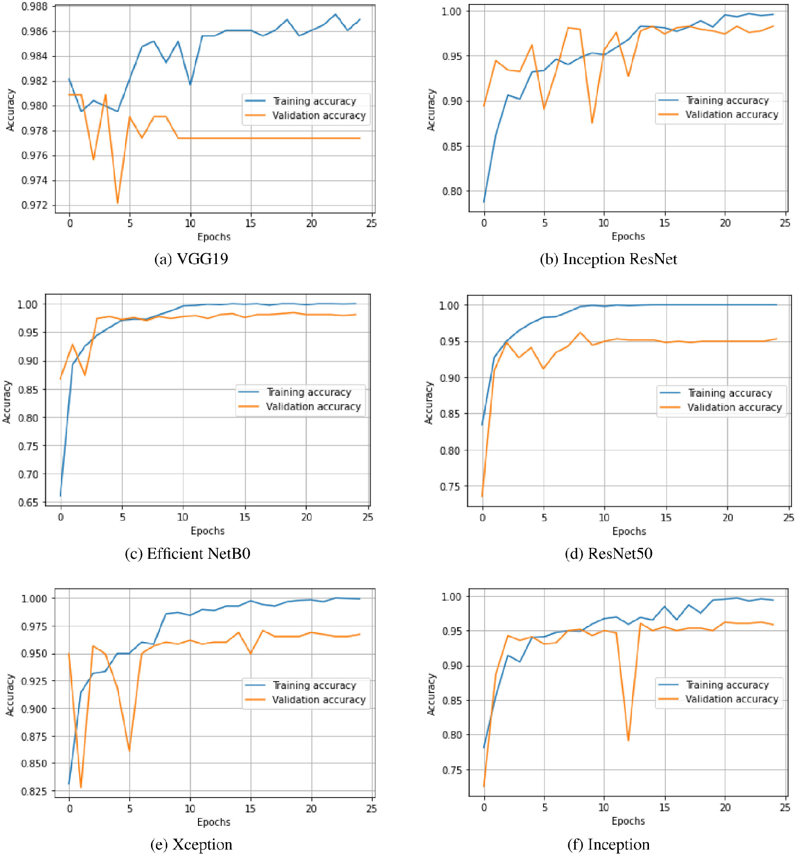
Figure 12.
Training and validation accuracy of the transfer learned models.
Both true-positive (TP) and true-negative (TN) predictions are accurate, while false-positive (FP) and false-negative (FN) are incorrect. Accuracy is indicated by a number between 0 and 1 and is often expressed as a percentage.
Precision is the ratio between the number of correct positives and the number of positives predicted by the classifier. Precision is a good choice for evaluation when we want to be very sure of our prediction. Precision can be determined using the confusion matrix as follows,
(4)
Precision indicates what proportion of predicted positives are actually positive [34].
Sensitivity (recall), also known as as true positive rate or hit rate, corresponds to the proportion of positive data points that are correctly classified as positive out of all positive data points. It is given by,
(5)
Sensitivity is a good choice for evaluation when we want to capture as many positive results as possible. Sensitivity indicates the proportion with which actual positive samples are correctly classified [34].
F1 score is basically the harmonic mean between sensitivity and precision (combining both sensitivity and precision) [35]. It is used to measure the accuracy of tests and is a direct indication of the performance of the model [31]. It is evaluated on the basis of the following equation.
(6)
The range of F1 scores is between 0 and 1, the aim being to get as close to 1 as possible. F1 is best when we have an uneven class distribution. We want a model that has both good precision and good sensitivity. The F1 score is a measure of the balance between precision and recall achieved by the proposed models. In general, the F1 score is low when either sensitivity or precision is low, and when both variables are high, it approaches one.
Figure 13.
Training and validation loss of the transfer learned models.
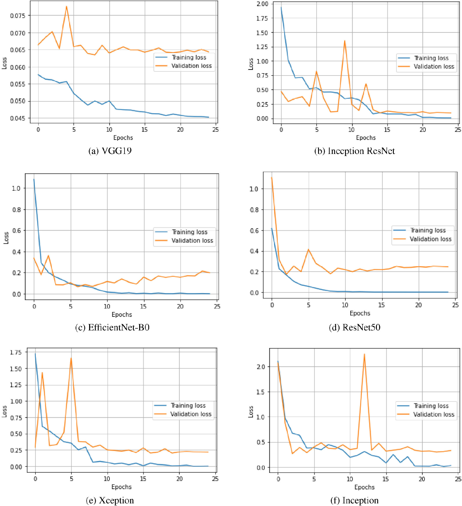
Figure 14.
Confusion matrix with the transfer learning models.
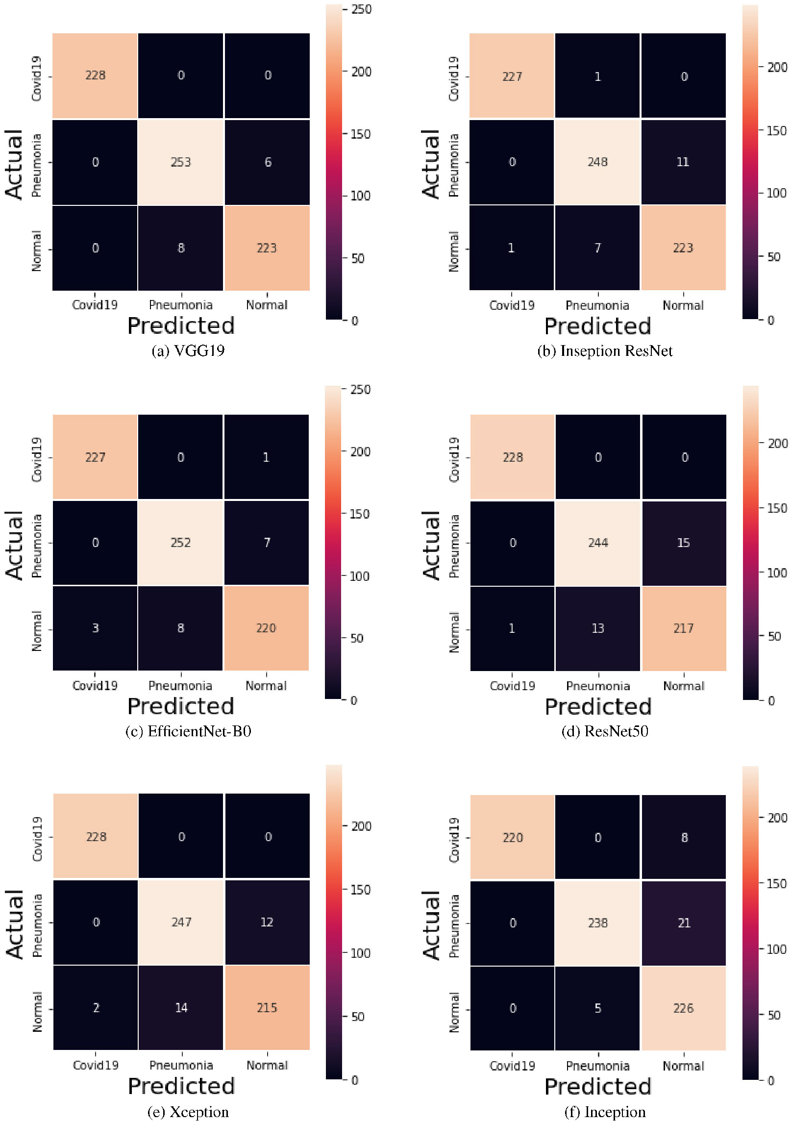
Figure 15.
Predicted X-ray images using VGG-19 model.
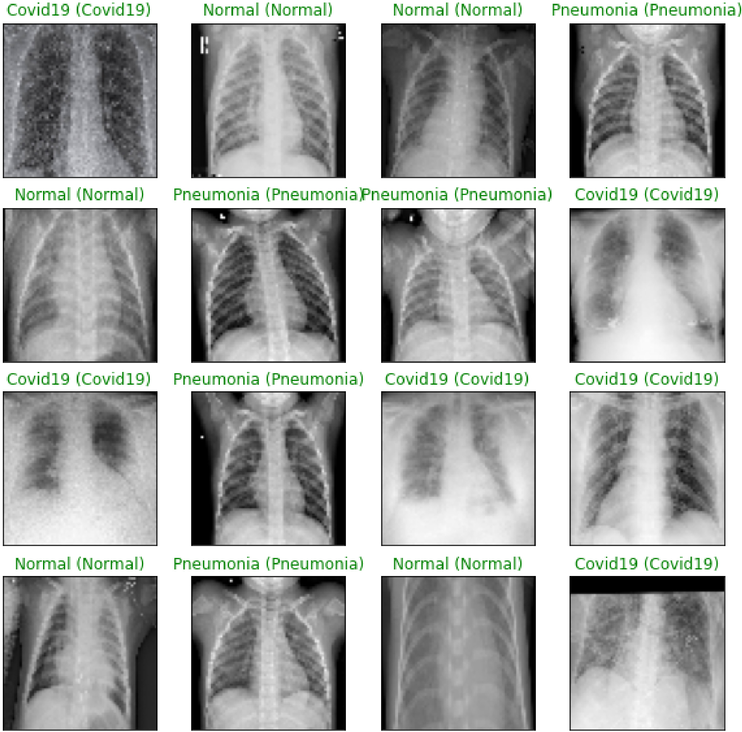
Figure 16.
Recognition accuracy versus model parameters.
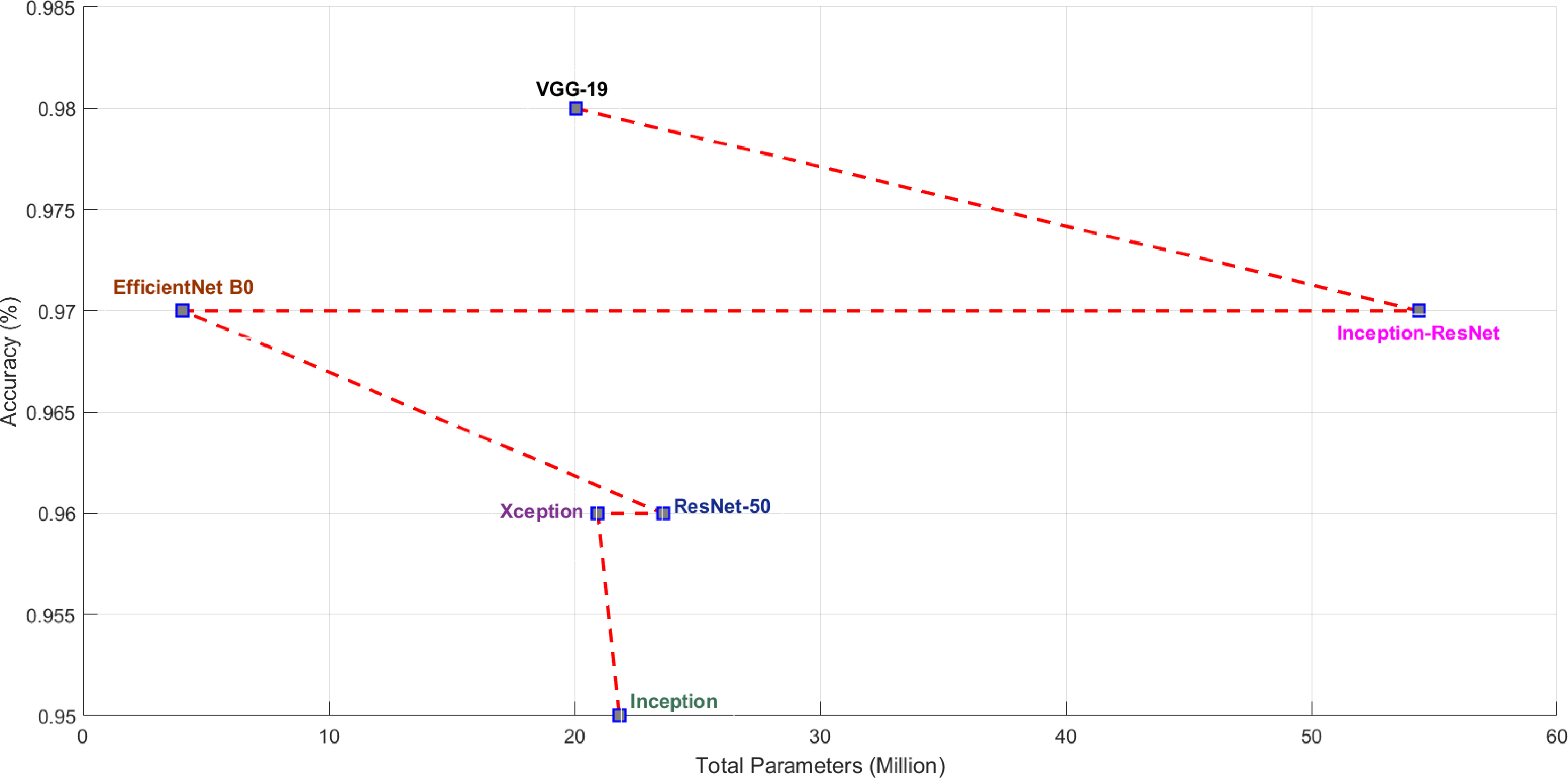
Table 2
Performance of the transfer learning models
| No | TL model | Health condition | Accuracy | Precision | Recall | F1 score |
|---|---|---|---|---|---|---|
| COVID-19 | 0.98 | 1.00 | 1.00 | 1.00 | ||
| 1 | VGG-19 | Non-COVID Pneumonia | 0.98 | 0.97 | 0.98 | 0.97 |
| Normal | 0.98 | 0.97 | 0.97 | 0.97 | ||
| COVID-19 | 0.97 | 1.00 | 1.00 | 1.00 | ||
| 2 | Inception-ResNet | Non-COVID Pneumonia | 0.97 | 0.97 | 0.96 | 0.96 |
| Normal | 0.97 | 0.95 | 0.97 | 0.96 | ||
| COVID-19 | 0.97 | 0.99 | 1.00 | 1.00 | ||
| 3 | EfficientNet-B0 | Non-COVID Pneumonia | 0.97 | 0.97 | 0.97 | 0.97 |
| Normal | 0.97 | 0.96 | 0.95 | 0.96 | ||
| COVID-19 | 0.96 | 1.00 | 1.00 | 1.00 | ||
| 4 | ResNet50 | Non-COVID Pneumonia | 0.96 | 0.95 | 0.94 | 0.95 |
| Normal | 0.96 | 0.94 | 0.94 | 0.94 | ||
| COVID-19 | 0.96 | 0.99 | 1.00 | 1.00 | ||
| 5 | Xception | Non-COVID Pneumonia | 0.96 | 0.95 | 0.95 | 0.95 |
| Normal | 0.96 | 0.95 | 0.93 | 0.94 | ||
| COVID-19 | 0.95 | 1.00 | 0.96 | 0.98 | ||
| 6 | Inception | Non-COVID Pneumonia | 0.95 | 0.98 | 0.92 | 0.95 |
| Normal | 0.95 | 0.89 | 0.98 | 0.93 |
Figure 17.
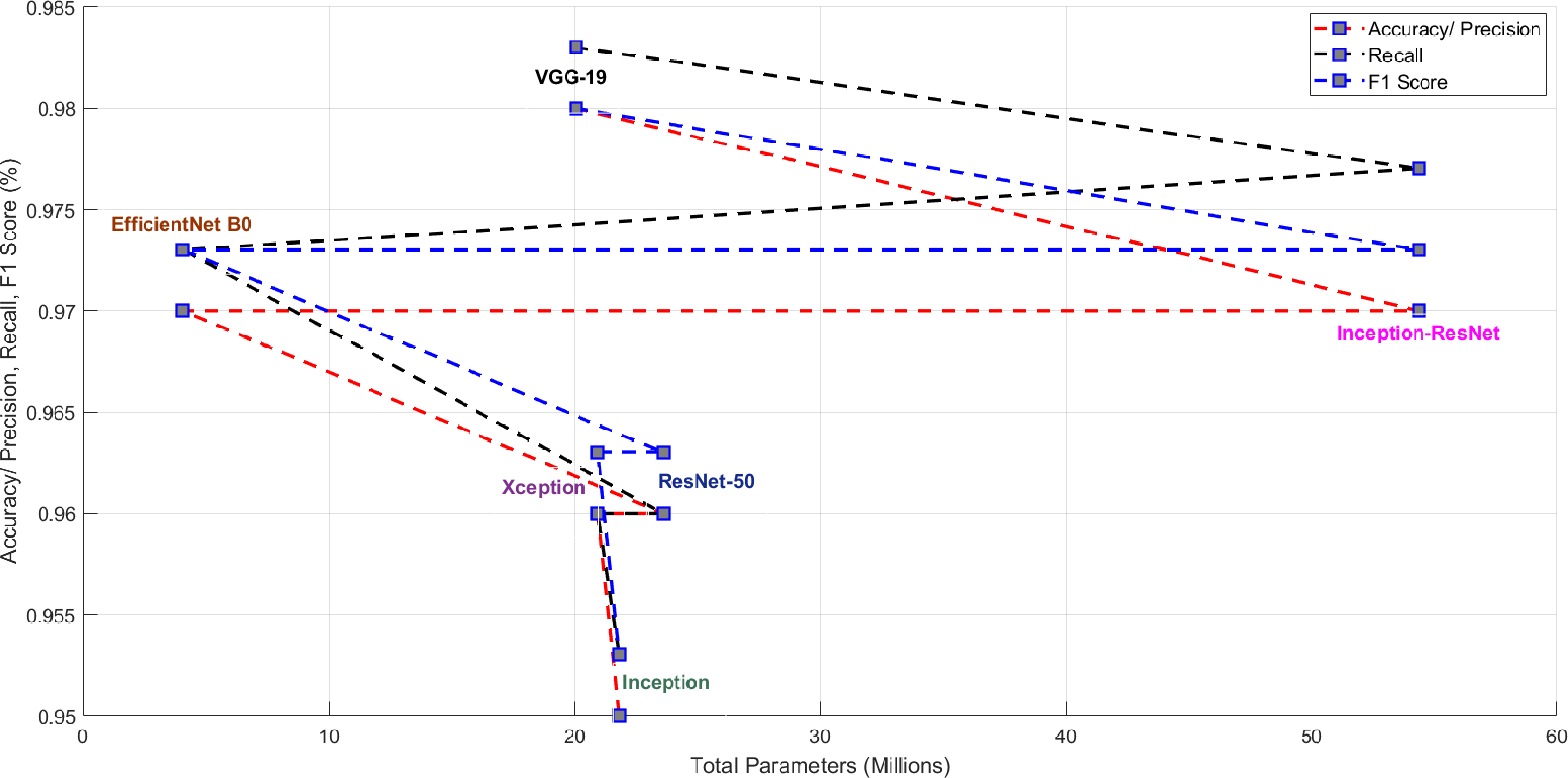
Model performance versus model parameters.
4.3Model comparison
This study investigated the performance of the well-known transfer learning for three-class categorisation of lung radiographs into COVID, pneumonia and normal. The trained dataset was first stored in an array with the respective labels. About 25 epochs were considered for training the models. The training and validation accuracy with all models is shown in Figs 12a and 12. Figures 13a and 13 show the training and validation loss of the presented models. The advantage of the transfer learning approach is its speed, as a lot of time is saved in the training process. Another notable advantage of the presented method is that it uses the best of the models in testing.
In the testing phase, test data was given to the best trained model and the model was evaluated on various metrics. Only 20% (714) of the total sample was considered for testing. The predicted results were compared with the actual results and the confusion matrix was constructed. Some radiographs predicted by the VGG-19 model are shown in Fig. 15. In Fig. 15 you can see the predicted patterns compared to the actual ground truth images. For each predicted image, the ground truth image is given in parentheses. The confusion matrix obtained with the models is summarised in Figs 14a and 14. The performance of the models in terms of accuracy, precision, recall and F1 score are shown in Table 2. Figures 16 and 17 show the performance measures of the classifiers in terms of the number of parameters used in each model. The computational complexity of the transfer learning models is shown in Figs 16 and 17.
From the results, among the prominent transfer learning models considered for the experiment, the VGG-19 model achieved the highest performance in three-class classification of radiographs into COVID, non-COVID pneumonia and normal. The VGG-19 model used 20,048,963 parameters to achieve an overall recognition accuracy of 98%. The time required to train the VGG-19 model in the Google Colab Platform with GPU was 25 minutes and 1.0 seconds for the test. The VGG-16 model used 14,739,267 parameters to achieve an overall recognition accuracy of 97%. The advantage of the VGG network is that it has a simple architecture and uses 33 convolutional filtres, the stride is Stride 1, uses the same padding and employs 2
The Inception ResNet-v2 model has the second highest accuracy. The model achieves the second highest recognition performance (Accuracy/Precision is 97%, Recall is 0.977 and F1 score is 0.973) by using the largest number of parameters (54,355,171) compared to all other models presented in this paper. The Inception ResNet-v2 model is precise and accurate but at the cost of maximum number of parameters and computational power (164 layers). It requires more training time compared to all other models. These experimental results also show that combining the Inception architecture with residual connections increases the performance of the Inception module. The Inception model shows a recognition accuracy/precision of 95%, a recall of 0.953 and an F1 score of 0.953, using 21,827,363 parameters in its model. The Inception architecture has been shown to give excellent results at low computational cost. When residual connections are used, the training of the Inception network is significantly accelerated. ResNet is about computational accuracy, while Inception is about computational cost. By combining Inception with ResNet, the performance of ResNet could be improved. ResNet is much deeper than VGG-19, but the model size is much smaller due to the use of global average pooling instead of fully connected layers – the model size for ResNet-50 is only 102 MB. The recognition accuracy/precision with the ResNet-50 model is 96%, while the Inception ResNet-v2 model improves the performance of ResNet-50 by updating the residual module to also use identity mappings.
Compared to the Inception ResNet-v2 and VGG-16 models, the EfficientNet-B0 model achieved similar performance with a relatively fewer number of parameters (4,058,534). The strategic scaling of depth, width and resolution in EfficientNet contributes to this performance advantage. The model had a recognition accuracy/precision of 97% with a recall and F1 score of 0.973. Compared to all other models considered, the training time for EfficientNet-B0 was the lowest. The Xception model has a recognition accuracy of 96%, a recall and F1 score of 0.960 and 0.963, respectively, and uses 20,959,787 parameters in its model. In the X-ray image dataset, Xception slightly outperforms Inception-v3. It has fewer model parameters than Inception, which makes it more computationally efficient. Inception V3 is the lowest performing model in the study, although its weights are only 96MB, which is less than VGG and ResNet.
The present study investigated the performance of widely used transfer learning models for three-class classification of radiographs into COVID-19, non COVID pneumonia and normal. The experimental results are presented in Figs 12, 13, 14 and Table 2. With the necessary effort, a database of reasonable size was created, containing about 1200 radiographs for COVID-19, non-COVID pneumonia and normal. In this study, a balanced dataset was considered to avoid network bias. The performance of the Deep Learning models was critically analysed.
5.Conclusions
One of the significant challenges in the automatic detection of COVID-19 from X-ray images is the selection of a suitable AI deep learning architecture. Therefore, this paper evaluates the performance of six highly efficient and accurate transfer learning models (VGG-19, Inception-ResNet, EfficientNet-B0, ResNet-50, Xception and Inception) for the early detection of COVID-19 on lung X-ray images. The present study considered the multiclass classification of radiographs into COVID-19, non-COVID pneumonia and normal. With a sample size of 3568 lung radiographs, only 80% were used for the training process. The performance of the transfer learning models was evaluated in terms of accuracy, sensitivity, precision and F1 score. Of the six transfer learning models, VGG-19 showed a high accuracy of 98%. The lowest accuracy was obtained with the Inception network (95%). The VGG-net, Inception ResNet and EfficientNet models are better when it comes to model accuracy. Compared to all six models, the Efficient model is lightweight as it requires fewer parameters and less training. In the future, the number of layers and nodes can be optimised and the number of parameters in each layer. The choice of the learning rate, the number of epochs, the intensity of regularisation, the network layers’ architecture, and the nodes’ optimisation require additional knowledge and skills. By incorporating information from different sources, more robust models can be created in the future.
References
[1] | WHO. World Health Organization Coronavirus Disease (COVID-19) Dashboard; (2021) . https//covid19.who.int/. |
[2] | Pulliam JRC, van Schalkwyk C, Govender N, von Gottberg A, Cohen C, Groome MJ, et al. Increased risk of SARS-CoV-2 reinfection associated with emergence of the Omicron variant in South Africa. MedRxiv. (2021) ; 376: (6593). https//www.medrxiv.org/content/early/2021/12/02/2021.11.11.21266068. |
[3] | Flick H, Arns BM, Bolitschek J, Bucher B, Cima K, Gingrich E, et al. Management of patients with SARS-CoV-2 infections and of patients with chronic lung diseases during the COVID-19 pandemic (as of 9 May 2020). Wiener klinische Wochenschrift. (2020) ; 132: (13): 365-386. doi: 10.1007/s00508-020-01691-0. |
[4] | Aburaed N, Panthakkan A, Al-Saad M, Mansoori SA, Ahmad HA. The Impact of Super Resolution on detecting Covid-19 from CT Scans using VGG-16 Based Learning. vol. 1828, IOP Publishing; (2021) . p. 012009. doi: 10.1088/1742-6596/1828/1/012009. |
[5] | Khatiwada S, Subedi A. Lung microbiome and coronavirus disease 2019 (COVID-19): Possible link and implications. Human Microbiome Journal. (2020) ; 17: : 100073. https//www.sciencedirect.com/science/article/pii/S245223172030004X. |
[6] | Allinovi M, Parise A, Giacalone M, Amerio A, Delsante M, Odone A, et al. Lung Ultrasound May Support Diagnosis and Monitoring of COVID-19 Pneumonia. Ultrasound in Medicine & Biology. (2020) ; 46: (11): 2908-2917. https//www.sciencedirect.com/science/article/pii/S0301562920303331. |
[7] | Ozturk T, Talo M, Yildirim EA, Baloglu UB, Yildirim O, Rajendra Acharya U. Automated detection of COVID-19 cases using deep neural networks with X-ray images. Computers in Biology and Medicine. (2020) ; 121: : 103792. https//www.sciencedirect.com/science/article/pii/S0010482520301621. |
[8] | Panthakkan A, Anzar SM, Mansoori SA, Ahmad HA. Accurate Prediction of COVID-19 (+) Using AI Deep VGG16 Model. In: 2020 3rd International Conference on Signal Processing and Information Security (ICSPIS); (2020) . pp. 1-4. |
[9] | Panthakkan A, Anzar SM, Mansoori SA, Ahmad HA. A novel DeepNet model for the efficient detection of COVID-19 for symptomatic patients. Biomedical Signal Processing and Control. (2021) ; 68: : 102812. https//www.sciencedirect.com/science/article/pii/S1746809421004092. |
[10] | Pan SJ, Yang Q. A Survey on Transfer Learning. IEEE Transactions on Knowledge and Data Engineering. (2010) ; 22: (10): 1345-1359. |
[11] | Tan C, Sun F, Kong T, Zhang W, Yang C, Liu C. A Survey on Deep Transfer Learning. In: Artificial Neural Networks and Machine Learning – ICANN 2018. Cham: Springer International Publishing; (2018) . pp. 270-279. |
[12] | Sahinbas K, Catak FO. 24 – Transfer learning-based convolutional neural network for COVID-19 detection with X-ray images. In: Data Science for COVID-19. Academic Press; (2021) . pp. 451-466. https//www.sciencedirect.com/science/article/pii/B9780128245361000034. |
[13] | Cohen JP, Morrison P, Dao L, Roth K, Duong TQ, Ghassemi M. Covid-19 image data collection: Prospective predictions are the future. arXiv preprint arXiv: 200611988v3. (2020) 06; https//arxiv.org/abs/2006.11988. |
[14] | Wang X, Peng Y, Lu L, Lu Z, Bagheri M, Summers RM. ChestX-ray8: Hospital-Scale Chest X-Ray Database and Benchmarks on Weakly-Supervised Classification and Localization of Common Thorax Diseases. In: Proceedings of the IEEE Conference on Computer Vision and Pattern Recognition (CVPR), (2017) , pp. 2097-2106. |
[15] | Narin A, Kaya C, Pamuk Z. Automatic detection of coronavirus disease (covid-19) using x-ray images and deep convolutional neural networks. Pattern Analysis and Applications. (2021) ; 24: (3): 1207-1220. doi: 10.1007/s10044-021-00984-y. |
[16] | Chouhan V, Singh SK, Khamparia A, Gupta D, Tiwari P, Moreira C, et al. A novel transfer learning based approach for pneumonia detection in chest X-ray images. Applied Sciences. (2020) ; 10: (2): 559. https//www.mdpi.com/2076-3417/10/2/559. |
[17] | Misra S, Jeon S, Lee S, Managuli R, Jang IS, Kim C. Multi-Channel Transfer Learning of Chest X-ray Images for Screening of COVID-19. Electronics. (2020) ; 9: (9): 1388. https//www.mdpi.com/2079-9292/9/9/1388. |
[18] | Taresh MM, Zhu N, Ali TAA, Hameed AS, Mutar ML. Transfer Learning to Detect COVID-19 Automatically from X-Ray Images Using Convolutional Neural Networks. International Journal of Biomedical Imaging. (2021) ; 2021: : 8828404. doi: 10.1155/2021/8828404. |
[19] | Maghdid HS, Asaad AT, Ghafoor KZ, Sadiq AS, Mirjalili S, Khan MK. Diagnosing COVID-19 pneumonia from x-ray and CT images using deep learning and transfer learning algorithms. In: Multimodal Image Exploitation and Learning 2021. vol. 11734. International Society for Optics and Photonics. SPIE; (2021) . pp. 99-110. doi: 10.1117/12.2588672. |
[20] | Polat Ç, Karaman O, Karaman C, Korkmaz G, Balcı MC, Kelek SE. COVID-19 diagnosis from chest X-ray images using transfer learning: Enhanced performance by debiasing dataloader. Journal of X-ray Science and Technology. (2021) ; 29: (1): 19-36. |
[21] | Kumar N, Gupta M, Gupta D, Tiwari S. Novel deep transfer learning model for COVID-19 patient detection using X-ray chest images. Journal of ambient intelligence and humanized computing. (2021) ; pp. 1-10. doi: 10.1007/s12652-021-03306-6. |
[22] | Aslan MF, Unlersen MF, Sabanci K, Durdu A. CNN-based transfer learning-BiLSTM network: A novel approach for COVID-19 infection detection. Applied Soft Computing. (2021) ; 98: : 106912. https//www.sciencedirect.com/science/article/pii/S1568494620308504. |
[23] | Abbas A, Abdelsamea MM, Gaber MM. 4S-DT: Self-supervised super sample decomposition for transfer learning with application to COVID-19 detection. IEEE Transactions on Neural Networks and Learning Systems. (2021) ; 32: (7): 2798-2808. |
[24] | Ahuja S, Panigrahi BK, Dey N, Rajinikanth V, Gandhi TK. Deep transfer learning-based automated detection of COVID-19 from lung CT scan slices. Applied Intelligence. (2021) ; 51: (1): 571-585. doi: 10.1007/s10489-020-01826-w. |
[25] | Al-Rakhami MS, Islam MM, Islam MZ, Asraf A, Sodhro AH, Ding W. Diagnosis of COVID-19 from X-rays Using Combined CNN-RNN Architecture with Transfer Learning. medRxiv. (2021) ; https//www.medrxiv.org/content/early/2021/08/09/2020.08.24.20181339. |
[26] | Jaiswal A, Gianchandani N, Singh D, Kumar V, Kaur M. Classification of the COVID-19 infected patients using DenseNet201 based deep transfer learning. Journal of Biomolecular Structure and Dynamics. (2021) ; 39: (15): 5682-5689. PMID: 32619398. doi: 10.1080/07391102.2020.1788642. |
[27] | Perumal V, Narayanan V, Rajasekar SJS. Detection of COVID-19 using CXR and CT images using Transfer Learning and Haralick features. Applied Intelligence. (2021) ; 51: (1): 341-358. doi: 10.1007/s10489-020-01831-z. |
[28] | Shalbaf A, Vafaeezadeh M, et al. Automated detection of COVID-19 using ensemble of transfer learning with deep convolutional neural network based on CT scans. International Journal of Computer Assisted Radiology and Surgery. (2021) ; 16: (1): 115-123. doi: 10.1007/s11548-020-02286-w. |
[29] | Singh M, Bansal S, Ahuja S, Dubey RK, Panigrahi BK, Dey N. Transfer learning – based ensemble support vector machine model for automated COVID-19 detection using lung computerized tomography scan data. Medical & Biological Engineering & Computing. (2021) ; 59: (4): 825-839. doi: 10.1007/s11517-020-02299-2. |
[30] | Simonyan K, Zisserman A. Very deep convolutional networks for large-scale image recognition. arXiv preprint arXiv: 14091556v6. (2014) . doi: 10.48550/arXiv.1409.1556. |
[31] | Glassner AS. Deep Learning: From Basics to Practice. vol. 1. The Imaginary Institute, Seattle, WA; (2018) . |
[32] | Aravindan A, Anzar S. Robust partial fingerprint recognition using wavelet SIFT descriptors. Pattern Analysis and Applications. (2017) ; 20: (4): 963-979. doi: 10.1007/s10044-017-0615-x. |
[33] | Powers DM. Evaluation: from precision, recall and F-measure to ROC, informedness, markedness and correlation. arXiv preprint arXiv: 201016061. (2020) . doi: 10.48550/arXiv.2010.16061. |
[34] | Grandini M, Bagli E, Visani G. Metrics for multi-class classification: an overview. arXiv preprint arXiv: 200805756. (2020) . doi: 10.48550/arXiv.2008.05756. |
[35] | Singh D, Kumar V, Kaur M. Classification of COVID-19 patients from chest CT images using multi-objective differential evolution – based convolutional neural networks. European Journal of Clinical Microbiology & Infectious Diseases. (2020) ; 39: (7): 1-11. doi: 10.1007/s10096-020-03901-z. |

