
Application of concepts of neighbours to knowledge graph completion1
Abstract
The open nature of Knowledge Graphs (KG) often implies that they are incomplete. Knowledge graph completion (a.k.a. link prediction) consists in inferring new relationships between the entities of a KG based on existing relationships. Most existing approaches rely on the learning of latent feature vectors for the encoding of entities and relations. In general however, latent features cannot be easily interpreted. Rule-based approaches offer interpretability but a distinct ruleset must be learned for each relation. In both latent- and rule-based approaches, the training phase has to be run again when the KG is updated. We propose a new approach that does not need a training phase, and that can provide interpretable explanations for each inference. It relies on the computation of Concepts of Nearest Neighbours (C-NN) to identify clusters of similar entities based on common graph patterns. Different rules are then derived from those graph patterns, and combined to predict new relationships. We evaluate our approach on standard benchmarks for link prediction, where it gets competitive performance compared to existing approaches.
1.Introduction
There is a growing interest for knowledge graphs (KG) as a way to represent and share data on the Web. The Semantic Web [2] defines standards for representation (RDF), querying (SPARQL), and reasoning (RDFS, OWL), and thousands of open KGs are available: e.g., DBpedia, Wikidata (formerly Freebase), YAGO, WordNet. The open nature of KGs often implies that they are incomplete, and a lot of work have studied the use of machine learning techniques to complete them.
The task of knowledge graph completion, a.k.a. link prediction [26], consists in predicting missing edges or missing parts of edges. It is therefore a form of machine learning. Suppose that film Avatar is missing a director in the KG, one wants to predict it, i.e. identify it among all KG nodes. The idea is to find regularities in the existing knowledge, and to exploit them in order to rank KG nodes. The higher the correct node is in the ranking, the better the prediction is. Link prediction was originally introduced for social networks with a single edge type (a single relation) [20], and was later extended to multi-relational data and applied to KGs [26]. Compared to the classical task of supervised classification, knowledge graph completion faces several challenges. First, there are as many classification problems as there are relations, which count in the hundreds or thousands in KGs. Second, for each relation, the number of “classes” is the number of different entities in the range of the relation, which typically counts in the thousands for relations like spouse or birthPlace. Third, some relations can be multi-valued, like the relation from films to actors.
In this paper, we report on extensive experimental results about a novel approach to knowledge graph completion that is based on Concepts of Nearest Neighbours (C-NN), which were introduced in [7], and applied to query relaxation in [8]. This paper is an extended version of [9] that reports on first results about the application of C-NNs to link prediction. In particular, the extension includes an analogical form of inference, and an extensive and deeper experimental evaluation. The C-NN approach introduces a symbolic form of k-NN (k Nearest Neighbours) where numerical distances are replaced by graph patterns that provide an intelligible representation of how similar two entities are.
Our hypothesis is that the partitioning of the KG entities into concepts of neighbours (see Section 5) provides a valuable basis for different kinds of inferences. We here focus on knowledge graph completion, i.e. the inference of the missing node of an incomplete edge. The combinatorial aspect of graph patterns over knowledge graphs is tackled by delaying their computation to inference time, which enables to bound the number of C-NNs by the number of entities, and in practice it is generally much smaller. The intensive knowledge-based computation at inference time is managed with in-memory KG indices (as is common in RDF stores), and any-time algorithms for both C-NN computation and inference. This allows us to scale up to standard link prediction benchmarks, which count up to 100K entities. Scaling further to millions of entities like in DBpedia or Wikidata is left for future work.
The contribution of this work is a novel approach to knowledge graph completion that has the following properties:
(1) it is a form of instance-based learning, i.e. it can perform inferences without training, and hence accommodate new data without re-training;
(2) it is a symbolic approach, i.e. it can provide explanations for each inference;
(3) it shows competitive performance on standard link prediction benchmarks.
The rest of the paper is organized as follows. Section 2 discusses related work on knowledge graph completion. Section 3 contains preliminaries about knowledge graphs and queries. Section 4 presents an overview of our approach. Section 5 recalls the definition of C-NNs, and their efficient computation. Section 6 presents our method to perform C-NN-based knowledge graph completion. Section 7 reports on positive experimental results on standard benchmarks (WN18, WN18RR, FB15k, FB15k-237), along with an in-depth analysis of results. Finally, Section 8 concludes and sketches future work.
2.Related work
Nickel et al. [26] published a “review of relational machine learning for knowledge graphs”, where link prediction is the main inference task. They identify two kinds of approaches that differ by the kind of model they use: latent feature models, and graph feature models. The former is by far the most studied one. Before going into details, it is useful to set the vocabulary as it is used in the domain. Nodes are called entities, edge labels are called relations, and edges are called triples
Latent feature models learn embeddings of entities and relations into low-dimensional vector spaces, and then make inferences about a triple
The latent feature models face two major drawbacks for their application to real settings. First, as they rely on the learning of entity embeddings, they cannot be applied to unseen entities, and the model has to be retrained whenever new entities or relations are introduced in the knowledge graph. Second, the predictions come without any explanation, and the meaning of learned latent features generally remain obscure. Given that it is unrealistic to expect high precision knowledge graph completion, simply because some of the missing information cannot be inferred from existing knowledge, human curation is necessary in practice. An explanation may comfort the curator in the veracity of the prediction, and could even be used to define automated inference rules.
Graph feature models, also called observed feature models, make inferences directly from the observed edges in the KG. Random walk inference [19] takes relation paths as features, and sets the feature values through random walks in the KG. The feature weights are learned by logistic regression for each target relation, and then used to score the candidate triples. The method has shown improvement over Horn clause generation with ILP (Inductive Logic Programming) [25]. AMIE+ [11] manages to generate such Horn clauses in a much more efficient way by designing new ILP algorithms tailored to KGs. They also introduce a novel rule measure that improves the inference precision under the Open World Assumption (OWA) that holds in KGs. A fine-grained evaluation [24] has shown that rule-based approaches are competitive with latent-based approaches, both in performance and in running time. AnyBURL [23] restricts to path-like Horn clauses, and employs an anytime bottom-up strategy for learning rules. It significantly improves performance compared to AMIE+, and gets close to the state-of-the-art of latent feature models. Graph feature models, especially rule-based approaches, offer the advantage to produce intelligible explanations for inferences, unlike the latent feature models. Moreover, they can be applied to unseen entities because inferences are based on the neighborhood of the entity in the knowledge graph, rather than on a learned embedding. However, they require a distinct training phase for each of the possibly many target relations, whereas the latent feature models are generally learned in one training phase. A drawback of both kinds of approaches is that new embeddings and new rulesets need to be learned whenever the KG is updated, which becomes a challenge for dynamic data.
Our approach relies on graph features but a key difference is that there is no training phase, and all the learning is done at inference time. It is therefore an instance-based approach rather than a model-based approach. Given an incomplete triple
3.Preliminaries
A knowledge graph (KG) is defined by a structure
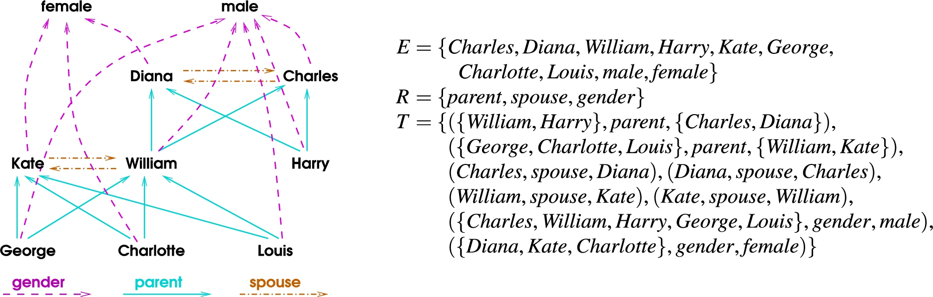
As a running example, Fig. 1 defines a small KG describing (part of) the British royal family (where
Fig. 1.
Example knowledge graph describing part of the British royal family.
Queries based on graph patterns play a central role in our approach as they are used to characterize the C-NNs, and can be used as explanations for inferences. There are two kinds of query elements: triple patterns and filters. A triple pattern
We now define the answer set that is retrieved by a query. A matching of a pattern P on a KG
4.Overview of the approach
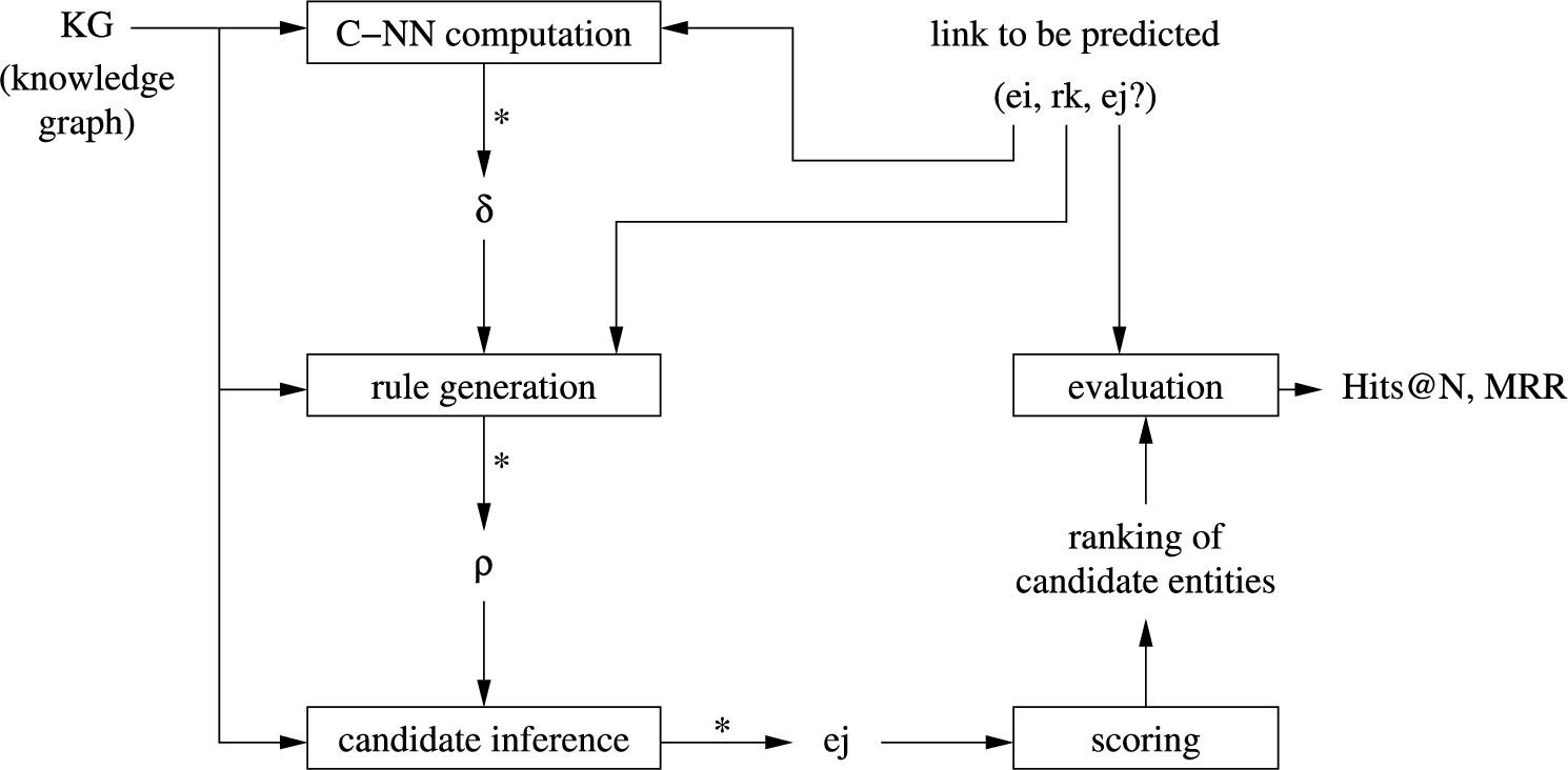
Fig. 2 shows a schematic overview of our approach. Given a knowledge graph and a triple
Fig. 2.
Overview of link prediction based on concepts of nearest neighbours.
5.Concepts of Nearest Neighbours (C-NN)
In this section, we shortly recall the theoretical definitions underlying Concepts of Nearest Neighbours (C-NN), as well as the algorithmic and practical aspects of their approximate computation under a given timeout. Further details are available in [7,8]. In the following definitions, we assume a knowledge graph
5.1.Theoretical definitions
We start by defining graph concepts, introduced in Graph-FCA [10], which is a generalization of Formal Concept Analysis (FCA) [12] to knowledge graphs. FCA concepts are a formalization of the classical theory of concepts in philosophy, where each concept has two related sides: the intension that characterizes what concept instances have in common, and the extension that enumerates those instances.
Definition 1.
A graph concept is defined as a pair
The most specific query
A concept
Instead of considering concepts generated by subsets of entities, we consider concepts generated by pairs of entities, and use them as a symbolic form of distance between entities.
Definition 2.
Let
For example, the above concept
A numerical distance
For example, the numerical distance is 5 between Charlotte and William (see
The number of conceptual distances
Definition 3.
Let
Table 1
Description of the 6 C-NNs of Charlotte in the royal family KG
| l | Sub-concepts | ||
| 1 | – | ||
| 2 | 1 | ||
| 3 | 1 | ||
| 4 | 3 | ||
| 5 | 2, 4 | ||
| 6 | 5 |
Fig. 3.
Venn diagram of the extensions of the 6 C-NNs of Charlotte, labelled by their numerical distance.
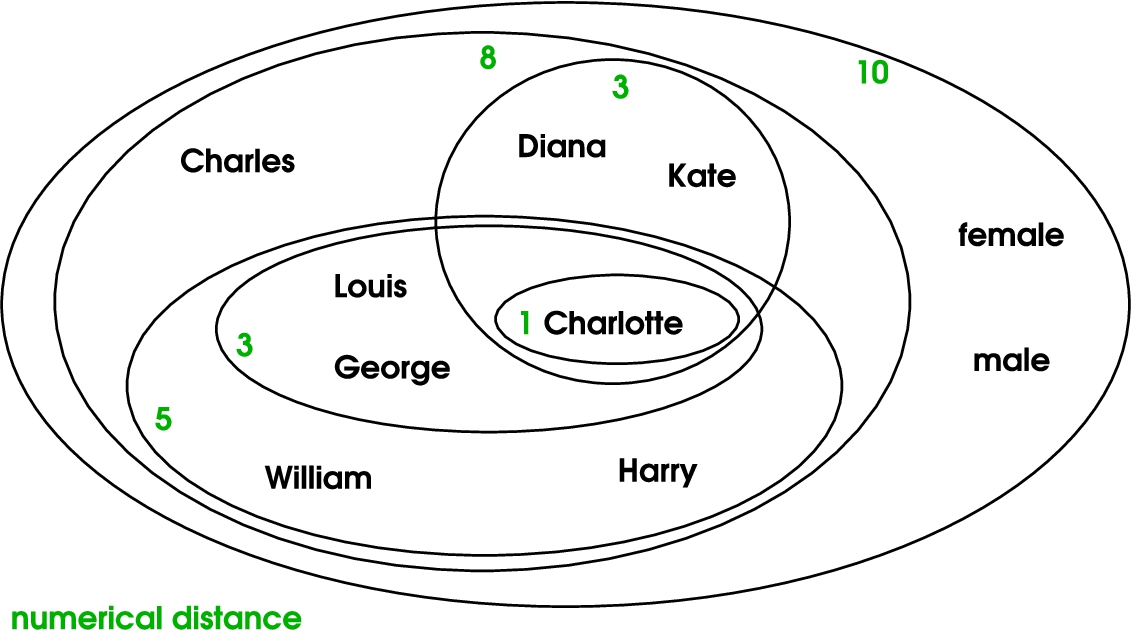
Table 1 lists the 6 C-NNs of Charlotte in the running example. Each row describes a concept of neighbours with its id, its extension, its intension, and its direct sub-concepts among the C-NNs. The bold part of extensions represent the proper extensions
Discussion. Given that
Compared to the use of numerical measures, like commonly done in k-NN approaches, C-NNs define a more subtle ordering of entities. First, because conceptual distances are only partially ordered, it can be that among two entities none is more similar than the other to the chosen entity e. This reflects the fact that there can be several ways to be similar to something, without necessarily a preferred one. For instance, who is most similar to Charlotte? Diana because she is also a female (C-NN
5.2.Algorithmic and practical aspects
We here sketch the algorithmic and practical aspects of computing the set
Each cluster
Algorithm 1
Partitioning algorithm for entity e in knowledge graph K
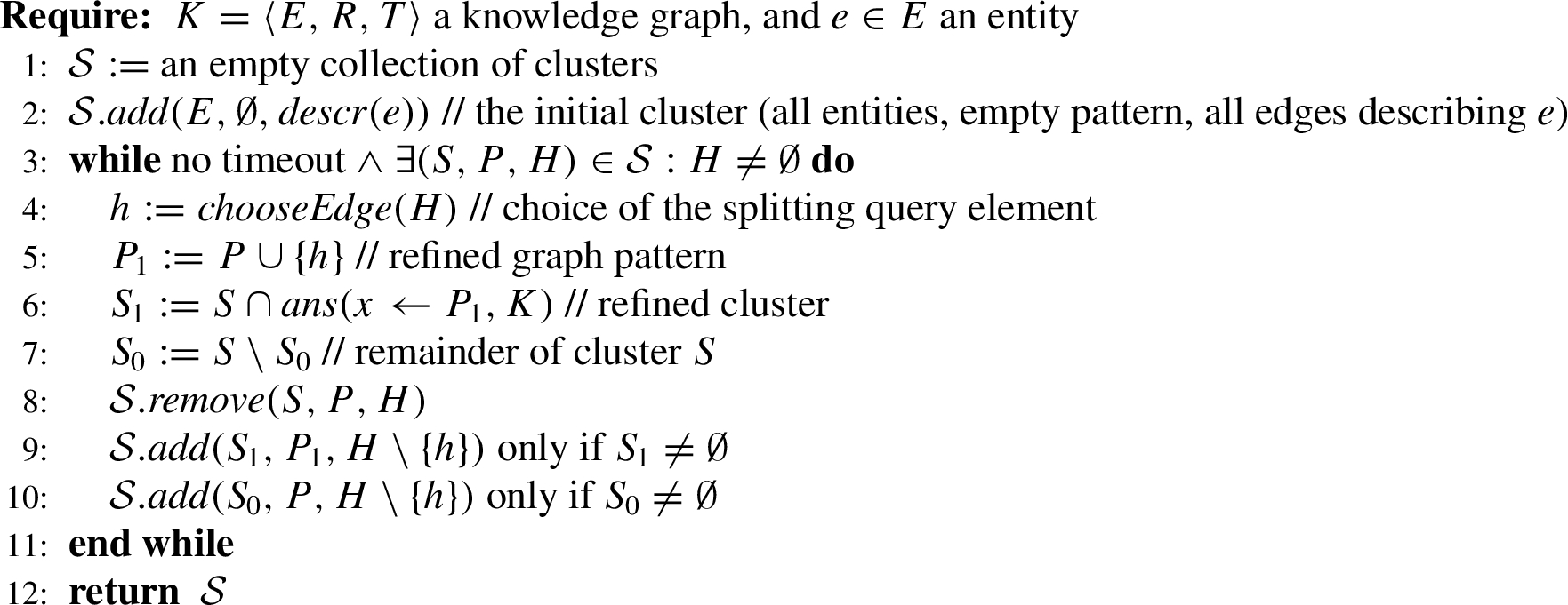
Algorithm 1 details the partitioning algorithm. Initially, there is a single cluster
Then at each iteration, any cluster S – with pattern P and set of candidate query elements H – is split in two clusters
Random: random choice among the valid elements;
Ordered: choice of equality elements first, then triple patterns whose relation is the least frequently used in P (novelty).
The new clusters are defined as follows:
Handling of RDF schema (RDFS). The implementation takes into account the domain knowledge expressed as RDF Schema axioms [16]. A special treatment is done for triples
Termination and efficiency. The above algorithm terminates because the set H (or its saturation in case of RDFS axioms) decreases at each split. However, in the case of large descriptions or large knowledge graphs, it can still take a long time. Now, previous experiments [8] show that most concepts are produced early, and that the rest of the time is spent at finding the last few concepts. Moreover, our algorithm is anytime because it can output a partition of entities at any time, and hence concepts of neighbours (possibly generalizations of them). It therefore makes sense to control runtime with a timeout parameter.
Actually, the above algorithm converges to an approximation of the C-NNs, in the sense that the conceptual distance may be still be an overestimate at full runtime for some entities. This is because graph patterns are constrained to be subsets of the description of e. In order to get exact results, the duplication of variables and their adjacent edges should be allowed, but this would considerably increase the search space.
Experiments on KGs with up to a million triples have shown that the algorithm can compute all C-NNs for descriptions of hundreds of edges in a matter of seconds or minutes. In contrast, query relaxation does not scale beyond 3 relaxation steps, which is insufficient to identify similar entities in most cases; and computing pairwise symbolic similarities does not scale to large numbers of entities. A key ingredient of the efficiency of the algorithm also lies in the notion of lazy join for the computation of answer sets of queries. In short, the principle is to compute
A last point to discuss is the scalability of C-NNs computation w.r.t. the KG size, i.e. what is the impact of doubling the number of entities. If we make the reasonable assumption that the new knowledge follows the same schema as the old knowledge (e.g., adding film descriptions to a film KG), then the impacts are that: (a) the query answers are two times larger, and (b) the number of C-NNs is somewhere between the same and the double, depending on the novelty of the new knowledge. As a consequence, if our objective is to compute a constant number of C-NNs for further inference, then it suffices to increase the timeout linearly with KG size.
6.Link prediction
The problem of link prediction is to infer a missing entity in a triple
6.1.C-NN-based inference
The principle of C-NN-based inference is to generate a ruleset for each concept of neighbours
(1) by-copy rules:
(2) by-analogy rules:
Inference by copy. The first kind of rules (by-copy rules) state that when an entity matches
Inference by analogy. The second kind of rules (by-analogy rules) state that when a pair of entities match
Comparison with rules in other approaches. The main difference with other rule-based approaches is that we only generate rules that are specific to the entity
6.2.Aggregation of inferences
Given an incomplete triple
The question addressed in this section is how to aggregate all inferences presented in previous section into a global ranking. Indeed, the known entity
Maximum Confidence (MC) score. This score is quite simple, and was shown effective in AnyBURL’s work. The score of entity
Dempster–Shafer (DS) score. This score is inspired by the work of Denœux [5], and adapted to our concepts of neighbours. Denoeux defines a k-NN classification rule based on Dempster–Shafer (DS) theory. Each k-nearest neighbour
We adapt Denoeux’s work to the inference of
Because in KGs a head entity can be linked to several tail entities through the same relation, we consider a distinct classification problem for each candidate tail entity
By applying Dempster–Shafer theory to combine the evidence from all rules ρ that predict entity
6.3.Inference algorithm and explanations
Algorithm 2 summarizes the full inference process in pseudo-code. Lines 1-3 initialises for each candidate entity the set of rules that infer it. Line 4 iterates over the C-NNs of entity
Algorithm 2
Inference and ranking of candidate entities
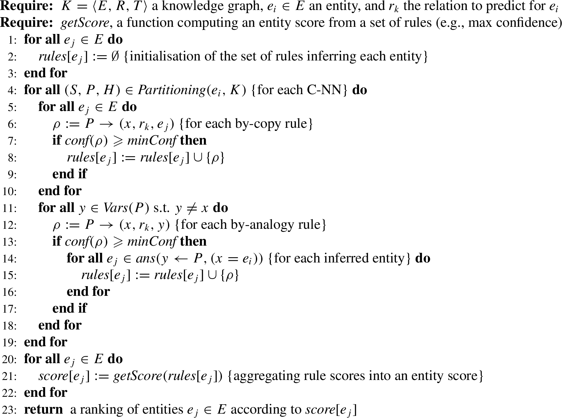
The algorithm can easily be extended to output for each inferred entity an explanation of why it was inferred. At Line 21, an explanation can be computed from the set of rules, in addition to the entity score. A simple form of explanation is to select the top-K rules according to the chosen score: confidence in the case of Maximum Confidence, and degree of belief in the case of Demster–Shafer. Each rule is directly interpretable in terms of entities and relationships (see Section 6.1). Their readability can be improved by pretty-printing or graphical representation of the graph pattern. In our implementation, the graph patterns are displayed in a Turtle-like notation by doing a tree traversal starting from variable x, which for recall denotes entity
7.Experiments
We here report on experiments comparing our approach to other approaches on several standard benchmarks for link prediction. We first present the methodology, and study the impact on performance of the different strategies and hyper-parameters of our approach. Then we report performance results on benchmarks with an in-depth analysis. Finally, we discuss example inferences and explanations, and present a fine-grained comparison with AnyBURL. The companion page22 provides access to the source code, the datasets, and the experiment main results and logs.
7.1.Methodology
Table 2
Statistics of datasets
| Dataset | Entities | Relations | Train edges | Valid. edges | Test edges |
| WN18 | 40943 | 18 | 141442 | 5000 | 5000 |
| WN18RR | 40559 | 11 | 86835 | 3034 | 3134 |
| FB15k | 14951 | 1345 | 483142 | 50000 | 59071 |
| FB15k-237 | 15541 | 237 | 272115 | 17535 | 20466 |
| Mondial | 2473 | 20 | 8456 | 570 | 701 |
Datasets. We use four datasets that are used in many work to evaluate the link prediction task (WN18, WN18RR, FB15k, FB15k-237), plus an additional dataset that we derived from the Mondial dataset [22]. Table 2 provides statistics about datasets (numbers of: entities, relations, train edges, validation edges, and test edges). WN18 and FB15k were introduced by Bordes et al. [4] for link prediction evaluation. WN18 is derived from a subset of WordNet, and FB15k from FreeBase. In later work, it was observed that many test triples had their inverse in the training set (e.g., hypernym is the inverse of hyponym in WordNet), and could be solved with very simple rules (e.g.,
We introduce Mondial as a subset of the Mondial database [22], which contains facts about world geography. We simplified it to the task of link prediction by removing labelling edges and edges containing dates and numbers, and by unreifying n-ary relations into binary relations. Triples whose relation is rdf:type were also removed from the validation and test sets because they do not represent proper links between entities. The dataset is available from the companion page. It is smaller than other datasets but it makes it easier to interpret results, and we use it to study the impact of the different strategies and hyper-parameters without introducing a bias in our evaluation on the classical benchmarks.
Task. We follow the same protocol as introduced in [4], and followed by subsequent work. The task is to infer, for each test triple, the tail entity from the head and the relation, and also the head entity from the tail and the relation. We call test entity the known entity, and missing entity the entity to be inferred. We evaluate the performance of our approach by using the same three measures as in [23]: MRR and
Method. Because our approach has no training phase we can use both train and validation datasets as examples for our instance-based inference. We consider a few alternative strategies:
The implementation of our approach has been integrated to SEWELIS as an improvement of previous work on the guided edition of RDF graphs [15]. A standalone program for link prediction is available from the companion page. We ran our experiments on Fedora 25, with CPU Intel(R) Core(TM) i7-6600U @ 2.60 GHz, and 16 GB DDR4 memory. So far, our implementation is simple and uses a single core, although our partitioning algorithm lends itself to parallelization. We have observed that in all our experiments the memory footprint, which includes the training and validation triples, remains under a few percents, i.e. a few hundreds MB. An alternative implementation33 for the computation of C-NNs has recently been developed as a Java library on top of the Jena Framework,44 in order to facilitate their reuse in other applications.
Baselines. We compare our approach to a number of historical or state-of-the-art latent-based approaches: DISTMULT [31], ANALOGY [21], KB_LR [13], R-GCN+ [29], ConvE [6], ComplEx-N3 [18], and CrossE [33]. We do so by choosing the same tasks and measures as in previous work because it was not possible for us to run them ourselves (no access to a GPU), and also because it allows for a fairer comparison (e.g., choice of hyper-parameters by authors). We also compare our approach to rule-based approaches: AMIE+ [11], RuleN [24], and AnyBURL [23]. Most performance results of the above approaches are reproduced from Meilicke et al. [23] (see Section 7.3 for details). We add yet another baseline Freq that simply consists in ranking entities
7.2.Impact of strategies and hyper-parameters and consistency of results
Table 3
Comparing MRR on Mondial with 12 different strategies
| by-copy | by-analogy | by-copy+analogy | ||||
| MC | DS | MC | DS | MC | DS | |
| Random | 28.6 | 16.9 | 42.4 | 41.3 | 45.5 | 44.2 |
| Ordered | 30.1 | 19.2 | 33.7 | 30.8 | 40.2 | 37.3 |
Impact of strategies. Table 3 compares the obtained MRR (in percents) on the Mondial dataset with different strategies. The timeout was set to 0.1 s for both C-NN computation and inference, and the maximum depth was set to 3. For recall, there are three axes composing the strategy:
choice of a splitting element: Random vs Ordered;
kinds of inference rules: by-copy vs by-analogy vs both (by-copy
aggregation of inferences: MC (max. confidence) vs DS (Dempster–Shafer).
Table 4
Evolution of performance and internal parameters with timeout
| Timeout (s) | Hits@1 | Hits@10 | MRR | nb. concepts | nb. inferred | max. conf |
| 0.001 | 15.7 | 31.8 | 21.2 | 3.7 | 103 | 0.20 |
| 0.01 | 32.3 | 51.3 | 38.9 | 11.9 | 211 | 0.42 |
| 0.1 | 38.6 | 59.1 | 45.5 | 35.0 | 311 | 0.57 |
| 1 | 39.3 | 63.7 | 47.3 | 89.2 | 351 | 0.66 |
Impact of timeout. Table 4 shows the evolution of a number of measures when timeout exponentially increases from 1 ms to 1 s. There are three performance measures (Hits@1, Hits@10, MRR), followed by three measures about the inference process, averaged over the test set: number of computed concepts of neighbours, number of inferred entities, and maximum confidence over all inferred entities. It can be observed that with only 1% of the largest timeout (timeout 0.01 s vs 1 s), the MRR is already at 82% of the larger MRR, and 60% of the inferred entities are obtained, despite the fact that only 13% of the concepts have been computed. This indicates that early approximations of concepts of neighbours are already informative. Furthermore, increasing the timeout and hence the number of concepts does not only improve MRR but also increases confidence in inferences as indicated by the steadily increasing maximum confidence.
Impact of description depth. We have observed that increasing description depth beyond 2–3 makes almost no significant difference on performance measures, as well as on the number of inferred entities and on the maximum confidence. In the following, we therefore stick to a maximum description depth equal to 3.
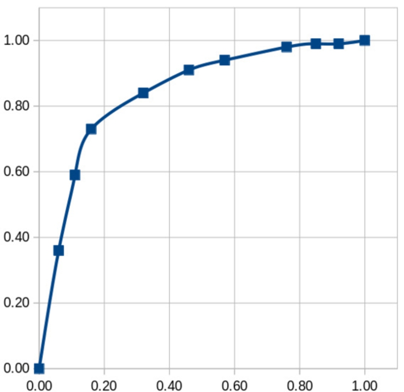
Fig. 4.
ROC curve of predicting Hits@1 correctness depending on maximum confidence threshold.
Consistency of results. To evaluate the consistency of the results of our approach, we perform two analyses on the Mondial dataset (with timeout = 0.1s). First, we analyze the variability of the performance measures by splitting the test set 10-fold. We observe that the standard error across the 10 folds is very small for all measures: e.g., 0.5% for MRR, around 1% for Hits@1 and Hits@10, and 0.4% for maximum confidence.
Second, we analyze the relevance of the maximum confidence by measuring how predictive it is about the correctness of predictions. Figure 4 shows the ROC curve for the classification task that consists in predicting whether the top entity in the filtered ranking is correct based on the hypothesis that its associated maximum confidence is above a threshold varying from 0 to 1. For example, with threshold at 0.70, the true positive rate is at 73% while the false positive rate is at 16%. The shape of the curve, as well as its AUC (Area Under Curve) equal to 84%, demonstrate the relevance of the maximum confidence to estimate the validity of predictions. This comes in complement with interpretable explanations for inferred entities in the form of rules.
7.3.Results on benchmarks
Table 5
Comparison of performance results on WN18 and WN18RR
| Approach | Source | WN18 | WN18RR | ||||
| H@1 | H@10 | MRR | H@1 | H@10 | MRR | ||
| Freq | 1.8 | 5.0 | 2.9 | 1.5 | 4.4 | 2.6 | |
| Latent-based | |||||||
| DISTMULT [31] | [29] | 70.1 | 94.3 | 81.3 | – | – | – |
| ANALOGY [21] | [21] | 93.9 | – | 94.2 | – | – | – |
| KB_LR [13] | [13] | – | 95.1 | 93.6 | – | – | – |
| R-GCN+ [29] | [23] | 69.7 | 96.4 | 81.9 | – | – | – |
| ConvE [6] | [23] | 93.5 | 95.5 | 94.2 | 39.0 | 48.0 | 46.0 |
| ComplEx-N3 [18] | [23] | – | 96.0 | 95.0 | – | 57.0 | 48.0 |
| CrossE [33] | [23] | 74.1 | 95.0 | 83.0 | – | – | – |
| Rule-based | |||||||
| AMIE+ [11] | [23] | 87.2 | 94.8 | – | 35.8 | 38.8 | – |
| RuleN [24] | [23] | 94.5 | 95.8 | – | 42.7 | 53.6 | – |
| AnyBURL [23] | [23] | 93.9 | 95.6 | 95.0 | 44.6 | 55.5 | 48.0 |
| C-NN (ours) | 96.7 | 97.2 | 96.9 | 44.4 | 51.9 | 46.9 | |
| C-NN − best other | |||||||
| C-NN − best other rule-based | |||||||
Table 6
Comparison of performance results on FB15k and FB15k-237
| Approach | Source | FB15k | FB15k-237 | ||||
| H@1 | H@10 | MRR | H@1 | H@10 | MRR | ||
| Freq | 14.3 | 28.5 | 19.2 | 17.5 | 35.6 | 23.6 | |
| Latent-based | |||||||
| DISTMULT [31] | [29] | 52.2 | 81.4 | 63.4 | 10.6 | 37.6 | 19.1 |
| ANALOGY [21] | [21] | 64.6 | – | 72.5 | – | – | – |
| KB_LR [13] | [13] | 74.2 | 87.3 | 79.0 | 22.0 | 48.2 | 30.6 |
| R-GCN+ [29] | [23] | 60.1 | 84.2 | 69.6 | 15.1 | 41.7 | 24.9 |
| ConvE [6] | [23] | 67.0 | 87.3 | 74.5 | 23.9 | 49.1 | 31.6 |
| ComplEx-N3 [18] | [23] | – | 91.0 | 86.0 | – | 56.0 | 37.0 |
| CrossE [33] | [23] | 63.4 | 87.5 | 72.8 | 21.1 | 47.4 | 29.9 |
| Rule-based | |||||||
| AMIE+ [11] | [23] | 64.7 | 85.8 | – | 17.4 | 40.9 | – |
| RuleN [24] | [23] | 77.2 | 87.0 | – | 18.2 | 42.0 | – |
| AnyBURL [23] | [23] | 80.4 | 89.0 | 83.0 | 23.0 | 47.9 | 30.0 |
| C-NN (ours) | 82.7 | 89.0 | 84.9 | 22.2 | 44.6 | 29.6 | |
| C-NN − best other | |||||||
| C-NN − best other rule-based | 0.0 | ||||||
Tables 5 and 6 compare the results of our approach (C-NN) to other approaches presented above as baselines on the four datasets WN18, WN18RR, FB15k, and FB15k-237. The baselines are organized in three groups: naive baseline Freq, latent-based approaches, and rule-based approaches. In each group, approaches are sorted by publication year. The source indicates which paper the results are taken from. The results for AnyBURL are those where 1000 s (largest available time) are allocated to the computation of rules. In the results of C-NN, the timeouts (computation of concepts + inference) are 1 + 1 s for WN datasets, and 1.5 + 0.5 s for FB datasets. The output logs of C-NN predictions and explanations are available from the companion page.
ComplEx-N3 clearly outperforms other approaches on all datasets except WN18 where C-NN outperforms other approaches on the three measures. C-NN comes second on FB15k, and remains close to the best approaches on WN18RR. On FB15k-237, the MRR delta is
Looking at the Freq baseline, it becomes visible how FB15k-237 is difficult because performance improvements over Freq are relatively small while they are huge on other datasets.
7.4.In-depth analysis of results
In this section, we refine the performance evaluation of our approach by analysing results w.r.t two criteria: (a) the kind of rule (by-copy vs by-analogy) that inferred the rank-1 predictions, (b) the characteristics of the relation to be predicted.
Table 7
Split of test sets depending on the kind of inference rule (by-copy vs by-analogy)
| Measure | WN18 | WN18RR | FB15k | FB15k-237 | ||||
| by-c | by-a | by-c | by-a | by-c | by-a | by-c | by-a | |
| Percent | 2% | 98% | 38% | 57% | 14% | 85% | 73% | 25% |
| Hits@1 | 15.0 | 98.7 | 15.2 | 67.8 | 37.0 | 91.0 | 26.2 | 12.2 |
| Hits@10 | 34.4 | 98.8 | 29.4 | 71.6 | 63.5 | 94.2 | 49.9 | 32.3 |
| MRR | 22.0 | 98.7 | 19.9 | 69.1 | 47.0 | 92.1 | 34.1 | 18.7 |
| max. conf | 0.24 | 0.96 | 0.28 | 0.70 | 0.60 | 0.88 | 0.61 | 0.66 |
Prediction by-copy vs by-analogy. We here analyze predictions according to the kind of the best rule, i.e. the rule with highest confidence, which contributed to decide the first entity in the generated ranking. For recall, there are two kinds of rules: by-copy rules and by-analogy rules (see Section 6.1). Table 7 shows the performance measures, and maximum confidence, on two subsets of the test set for each dataset, depending on the kind of the best rule. Line “percent” gives the relative size of those subsets. The two percentages may not sum up to 100% because for some test cases, no prediction could be made: e.g., all predicted entities are already known to hold, and are therefore filtered out.
The balance between by-copy and by-analogy can be explained by the nature of each dataset. In WN18 and FB15k it is well known that most test triples can be inferred from an inverse triple, which is well captured with by-analogy rules: e.g.,
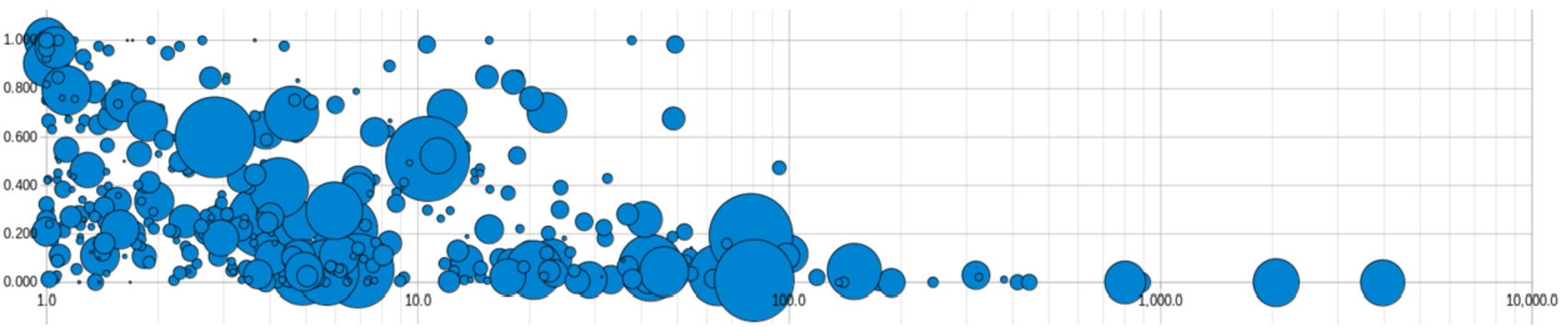
Fig. 5.
MRR as a function of relation degree. Bubble sizes are proportional to relation frequency.
Results depending on relation characteristics. Relations are not all alike in knowledge graphs. They vary in frequency, and whether they are functional or multi-valued. We here define the frequency of a relation r as the number of test triples using it; and its degree as the average number of tail entities per head entity in the training set. When the degree equals (or is closed to) 1, the relation is said functional, otherwise it is said multi-valued. As the benchmarks imply to predict both the tail from the head, and the head from the tail, we also consider inverse relations. Their frequency is the same, and their degree is the average number of head entities per tail entity. The degree of the inverse relation is unrelated to the degree of the relation, and all combinations are possible, i.e. 1–1, n–1, 1–n, and n–n relations.
Figure 5 shows a bubble plot of the 224 relations and their inverses, which are found in the test set of FB15k-237, the most challenging dataset. Each bubble is positioned according to its degree (ranging from 1 to 4000), and to the MRR of its predictions (ranging from 0 to 1). The bubble size reflects the frequency of the relation, and hence its weight in the global performance measures. Several observations can be made. First, the relations cover a wide range of frequencies and degrees, and there are no obvious correlation between those two dimensions. Second, there is a clear tendency that the higher the degree, the lower the MRR, i.e. multi-valued relations are harder to predict than functional relations. However, many relations stand under and above this tendency. Some relations have a low MRR despite a low degree (e.g., place of birth); and some relation succeeds to have a high MRR despite degrees up to 50 (e.g., inverse of food nutrient with degree = 15). Examples of frequent relations with high MRR are: people nationality (degree = 1.1, MRR = 79.3), people gender (degree = 1, MRR = 90.4), topic webpage category (degree = 1, MRR = 100), marriage type of union (degree = 1.1, MRR = 100), award winners ceremony (degree = 12, MRR = 71.4), and its inverse (degree = 22, MRR = 70.1).
Scalability w.r.t. the size of the knowledge graph. The scalability of the C-NN approach is difficult to evaluate because the runtime is determined by the user-given timeouts. It can only be evaluated by comparing the prediction performance for KGs of different sizes. However, the prediction performance cannot be compared easily between different datasets because inference difficulty varies from one dataset to another. Even starting from one large KG and using subgraphs of different sizes is tricky if one wants to keep the same inference difficulty. Synthetic KGs may be useful for benchmarking the scalability of query or reasoning engines [3,14] but they may not have enough regularities for the task of link prediction. We propose the following methodology to give some hint on the scalability of our approach. We consider an additional link prediction dataset, YAGO03-10 [6], that is similar in contents to the Freebase datasets but with about 10 times more entities (123K). According to our discussion at the end of Section 5, the timeout should increase linearly with the number of entities. We therefore ran our approach with timeouts 15 + 5 s, and we checked if C-NN’s performance remains competitive with AnyBURL’s performance on YAGO3 (available in [23], with timeout = 1000 s like above). Estimating on 10% of test instances (out of 10000), we obtain the following results.
| Approach | H@1 | H@10 | MRR |
| AnyBURL | 42.9 | 63.9 | 49 |
| C-NN | 42.4 ± 1.5 | 67.8 ± 1.4 | 51.2 ± 1.4 |
The differences are comparable with those of other datasets, hence supporting the linear scaling rule.
Now, the consequence of that linear scaling is that our approach cannot yet be applied in practice to very large KGs with millions of entities, like DBpedia or Wikidata, as the timeout per inference would have to be increased to non-practical values (about 15 min on DBpedia). In order to achieve this goal, it will be necessary to compute more concepts of neighbours in less time. Optimization will not be enough, and it will be necessary to find robust sampling strategies: to compute C-NNs on a representative subset of entities, to select the relevant part of entity descriptions in the partitioning process, and to estimate the confidence of rules without computing all pattern matchings.
7.5.Example inferences and explanations
In this section, we look at example inferences in order to discuss the explainability of our approach. Note that further work is required to make explanations easier to use, and that our objective is here to show the potential of our approach, and the limits of the current implementation. We here consider inferences for the Mondial datasets because they are easier to read. Indeed, the Freebase and WordNet datasets use opaque identifiers for entities (e.g., 03735637 in WordNet, 05h43ls in Freebase), while Mondial uses clear URIs (e.g., http://www.semwebtech.org/mondial/10/country/ANG for Angola). In the next section we discuss inferences on FB15k-237 in comparison to AnyBURL. We describe below four correct and one incorrect inferences. Those are not cherry-picked. They are simply the top five inferences in the experiment log available on the companion page (only considering 0.1 + 0.1 s timeout). In the following, support and confidence measures are abbreviated as ‘supp’ and ‘conf’.
(1) The (missing) neighbors countries of Angola are correctly predicted to be Zambia and Zaire (conf = 0.91) by the following by-analogy rule (supp = 85, conf = 0.91). Subsequent predictions have much lower confidences: South Sudan and Cameroon (conf = 0.41).
This rule is a specialization of the rule(2) Sweden is correctly predicted to be encompassed in Europe by the following by-value rule (supp = 25, conf = 0.56). The subsequent prediction is America (conf = 0.36).
This rule says that a country x is in Europe if it has a language and a neighbor country, and if it contains a lake and a mountain. Obviously, this is not a generally valid rule, as its confidence shows, but its inferences are still valid in the majority of cases. It is interesting to see that our approach can not only make logical inferences like in the first example, but also statistical inferences based on best guess rules.(3) Islay is correctly predicted to belong to Inner Hebrides (conf = 0.34 0.34 0.31) by the following top-1 by-analogy rule (supp = 54, conf = 0.34), and two other rules (not shown, conf = 0.34 and conf = 0.31). There are five subsequent predictions (all UK islands) with same first and second confidences but lower third confidence, then Canares (conf = 0.29), Lesser Antilles (conf = 0.27).
This rules says that an island x belongs to islands y if x shares a location (here, UK) with another island z that belongs to y, and x is located in the Atlantic Ocean. Apart from the specialization to the Atlantic Ocean, this rules makes sense because if two islands are located in a same place, e.g. a same country, there is a good chance that they belong to the same islands. However, this is not precise enough, like here where UK islands belong to 5 different islands (Inner Hebrides, Outer Hebrides, Shetlands, …). The top-3 rules are required to discriminate between them. This demonstrates the value of the maximum confidence measure that makes use of all rule confidences in ranking. Note that without the additional rules, the correct entity would still be at a small rank, here 5th in the worst case.(4) Matternhorn is correctly predicted to be located in Switzerland (conf = 0.42 0.36) by the following top-1 by-analogy rule (supp = 153, confs = 0.42) and another rule (not shown, conf = 0.36). Subsequent predictions are France (conf = 0.42 0.27), Austria (conf = 0.42 0.14), Germany (conf = 0.42 0.11).
This rule is similar to the previous one. In short, it says that two mountains that belong to the same mountain range tends to be located in the same place (typically a country). The confidence is 0.42 so that there are many exceptions but the support is high (supp = 153). Similarly to the previous example, an additional rule was required to discriminate with neighbor countries.(5) The Baltic sea is incorrectly predicted to have an inflow from Goetaaelv (conf = 0.33) by the following by-copy rule (supp = 1, conf = 0.33), instead of the expected Narva and Dalaelv (conf = 0.03), which are predicted at ranks 274 and 302. Goetaaelv flows into a neighbor sea (Kattegat) of the Baltic sea but not in the Baltic sea proper.
This rule is very specific, and its support is only 1. It is clear that such an explanation should not be trusted blindly. Laplace smoothing helped lower its confidence from 1 downto 0.33 but no better rule was found here. Note however that rules with low support can still be useful sometimes when they retrieve very similar entities from which valid inferences can be drawn.
7.6.Detailed comparison with AnyBURL
In this section, we detail the comparison with predictions made by AnyBURL.55 Indeed, AnyBURL is the state-of-the-art among rule-based approaches. The main question we answer here is: How predictions differ between C-NN and AnyBURL? Table 8 gives for the four datasets the distribution of test instances into four cases depending on the Hits@1 success of each approach (C-NN and AnyBURL). If the rank-1 predicted entity is correct, then Hits@1 equals 1, otherwise it equals 0. Case 1/1 means that both approaches are correct, case 1/0 means that C-NN is correct but not AnyBURL, etc. The four cases sum up to 100%.
We consider the null hypothesis that if one approach has lesser performance, then its set of correct predictions is a subset of the correct predictions of the other approach. For instance, on FB15k-237 where AnyBURL is better, we expect that case 0/1 is empty. This is rejected in all four datasets. For instance, on FB15k-237, C-NN is the only correct approach for 4.7% test instances, which amounts to 1918 test instances. Those results demonstrate that C-NN and AnyBURL can complement each other, and that improvement of state-of-the-art performances remains possible. This is made explicit in the last two columns that allow to compare Hits@1 of the best of the two approaches and the best ensemble of the two (union of correct predictions).
Table 8
Distribution of test instances depending of Hits@1 success of C-NN and AnyBURL. The last two columns give the average Hits@1 first for the best of the two approaches, and second for the best ensemble
| Dataset | nb. test | H@1 C-NN/H@1 AnyBURL | H@1 | ||||
| 1/1 | 1/0 | 0/1 | 0/0 | Best of two | Best ensemble | ||
| WN18 | 10100 | 93.2 | 3.4 | 0.9 | 2.5 | 96.6 | 97.5 |
| WN18RR | 6268 | 41.3 | 3.1 | 3.6 | 52.0 | 44.9 | 48.0 |
| FB15k | 118142 | 75.3 | 7.4 | 5.5 | 11.8 | 82.7 | 88.2 |
| FB15k-237 | 40932 | 17.5 | 4.7 | 6.2 | 71.6 | 23.7 | 28.4 |
We now detail a few test instances where C-NN and AnyBURL differ (cases 1/0 and 0/1). The analysis is limited by the fact that AnyBURL’s code does not output rules as explanations for predictions (although the code could be modified to do so). Here are a few test instances where C-NN succeeds while AnyBURL fails:
Wichita falls were correctly predicted to have Central Time Zone because it is contained in Texas (by-copy rule, support = 31, confidence = 0.79);
Joe Shuster was correctly predicted to have written “Superman II: The Richard Donner Cut” because he has produced a story that was honored for the film, and he won some award (by-analogy rule, support = 5, confidence = 0.36);
Joe Shuster was also correctly predicted to live in Cleveland because he has produced the story “Superman II” (by-copy rule, support = 1, confidence = 0.33). Here the explanation is not so convincing because of the very low support;
Film “Good Will Hunting” was correctly predicted to have two crew roles “make-up artist” and “special effects supervisor” because it was nominated for the “Satellite Award for Best Original Screenplay” (by-copy rule, support = 16, confidence = 0.78). Here the rule is probably overly specific as most films probably have the two crew roles, not only those nominated for the “Satellite Award…”. Post-processing would be useful to remove the redundant parts.
Now, here are test instances where C-NN fails while AnyBURL succeeds. In each instance, we give the best C-NN rule, which fails, and then the “successful C-NN rule”, i.e. the highest-confidence rule found by our approach that infers the correct entity.
Lily Tomlin was incorrectly predicted to be nominated for TV series “Murphy Brown”, instead of “The West Wing” (predicted 2nd), because he is an actor of the TV series, and won an award (by-analogy rule, support = 364, confidence = 0.53). The successful rule predicts “The West Wing” because he was nominated along with Joshua Malina (by-copy rule, support = 14, confidence = 0.50);
Film “Life is beautiful” was incorrectly predicted to have genre Italian, instead of War Film (predicted 8th), because it appears on the title list of the Netflix genre “Italian” (by-analogy rule, support = 393, confidence = 0.56). The successful rule predicts War Film because it was produced in Italy (by-copy rule, support = 14, confidence = 0.25).
8.Conclusion
We have shown that a symbolic approach to the problem of knowledge graph completion can be competitive with state-of-the-art approaches, both latent-based and rule-based. This comes with the major advantage that our approach can provide detailed explanations for each inference, in terms of the graph features. Compared to rule-based approaches, which can provide similar explanations, we follow an instance-based approach, and hence avoid the need for a training phase that can be costly in runtime and memory (rule mining), in particular with dynamic data. Moreover, our rule language bias is weaker by allowing arbitrary conjunctive rules with constants, while avoiding a combinatorial explosion thanks to our instance-based approach and our partitioning algorithm. Our approach is analogous to classification with k-nearest neighbours but our distances are defined as partially-ordered graph concepts instead of numbers.
There are many tracks for future work. Extending graph patterns with n-ary relations and richer filters over numbers, dates, etc. Optimizing and scaling the computation of C-NNs by finding good strategies to drive the partitioning process, or by parallelizing it. Improving the selection and display of rules as explanations. Evaluating our approach on other datasets, and other inference tasks.
Notes
2 Companion page: http://www.irisa.fr/LIS/ferre/pub/link_prediction2020/.
5 Detailed predictions for state-of-the-art latent-based approaches are not available, and specific hardware (GPUs) is required to run them in a reasonable amount of time.
Acknowledgements
I kindly thank the reviewers for their insightful remarks, and valuable suggestions, which contributed to significantly improve this paper.
References
[1] | R. Agrawal, R. Srikant et al., Fast algorithms for mining association rules, in: Int. Conf. Very Large Data Bases (VLDB), Vol. 1215: , (1994) , pp. 487–499, http://vldb.org/conf/1994/P487.PDF. |
[2] | T. Berners-Lee, J. Hendler and O. Lassila, The semantic web, Scientific American 284: (5) ((2001) ), 34–43. doi:10.1038/scientificamerican0501-34. |
[3] | C. Bizer and A. Schultz, The berlin sparql benchmark, Int. J. Semantic Web and Information Systems 5: (2) ((2009) ). doi:10.4018/jswis.2009040101. |
[4] | A. Bordes, N. Usunier, A. Garcia-Duran, J. Weston and O. Yakhnenko, Translating embeddings for modeling multi-relational data, in: Advances in Neural Information Processing Systems, (2013) , pp. 2787–2795. |
[5] | T. Denœux, A k-nearest neighbor classification rule based on Dempster–Shafer theory, IEEE Trans. Systems, Man, and Cybernetics 25: (5) ((1995) ), 804–813. doi:10.1109/21.376493. |
[6] | T. Dettmers, P. Minervini, P. Stenetorp and S. Riedel, Convolutional 2D knowledge graph embeddings, in: Conf. Artificial Intelligence (AAAI), S.A. McIlraith and K.Q. Weinberger, eds, AAAI Press, (2018) , pp. 1811–1818, https://www.aaai.org/ocs/index.php/AAAI/AAAI18/paper/viewPaper/17366. |
[7] | S. Ferré, Concepts de plus proches voisins dans des graphes de connaissances, in: Ingénierie des Connaissances (IC), (2017) , pp. 163–174, https://hal.archives-ouvertes.fr/hal-01570277. |
[8] | S. Ferré, Answers partitioning and lazy joins for efficient query relaxation and application to similarity search, in: Int. Conf. the Semantic Web (ESWC), A. Gangemi et al., eds, LNCS, Vol. 10843: , Springer, (2018) , pp. 209–224. doi:10.1007/978-3-319-93417-4_14. |
[9] | S. Ferré, Link prediction in knowledge graphs with concepts of nearest neighbours, in: The Semantic Web (ESWC), P. Hitzler et al., eds, LNCS, Vol. 11503: , Springer, (2019) , pp. 84–100. doi:10.1007/978-3-030-21348-0_6. |
[10] | S. Ferré and P. Cellier, Graph-FCA: An extension of formal concept analysis to knowledge graphs, Discrete Applied Mathematics 273: ((2019) ), 81–102. doi:10.1016/j.dam.2019.03.003. |
[11] | L. Galárraga, C. Teflioudi, K. Hose and F. Suchanek, Fast rule mining in ontological knowledge bases with AMIE+, Int. J. Very Large Data Bases 24: (6) ((2015) ), 707–730. doi:10.1007/s00778-015-0394-1. |
[12] | B. Ganter and R. Wille, Formal Concept Analysis – Mathematical Foundations, Springer, (1999) . doi:10.1007/978-3-642-59830-2. |
[13] | A. García-Durán and M. Niepert, KBlrn: End-to-end learning of knowledge base representations with latent, relational, and numerical features, in: Conf. Uncertainty in Artificial Intelligence (UAI), A. Globerson and R. Silva, eds, AUAI Press, (2018) , pp. 372–381, http://auai.org/uai2018/proceedings/papers/149.pdf. |
[14] | Y. Guo, Z. Pan and J. Heflin, LUBM: A benchmark for OWL knowledge base systems, Journal of Web Semantics: Science, Services and Agents 3: (2–3) ((2005) ), 158–182. doi:10.1016/j.websem.2005.06.005. |
[15] | A. Hermann, S. Ferré and M. Ducassé, An interactive guidance process supporting consistent updates of RDFS graphs, in: Int. Conf. Knowledge Engineering and Knowledge Management (EKAW), A. ten Teije et al., eds, LNAI, Vol. 7603: , Springer, (2012) , pp. 185–199. doi:10.1007/978-3-642-33876-2_18. |
[16] | P. Hitzler, M. Krötzsch and S. Rudolph, Foundations of Semantic Web Technologies, Chapman & Hall/CRC, (2009) . ISBN 9781420090505. doi:10.1201/9781420090512. |
[17] | C.A. Hurtado, A. Poulovassilis and P.T. Wood, Query relaxation in RDF, in: Journal on Data Semantics X, S. Spaccapietra, ed., LNCS, Vol. 4900: , Springer, (2008) , pp. 31–61. doi:10.1007/978-3-540-77688-8_2. |
[18] | T. Lacroix, N. Usunier and G. Obozinski, Canonical tensor decomposition for knowledge base completion, in: Int. Conf. Machine Learning (ICML), J.G. Dy and A. Krause, eds, Proceedings of Machine Learning Research, Vol. 80: , PMLR, (2018) , pp. 2869–2878, http://proceedings.mlr.press/v80/lacroix18a.html. |
[19] | N. Lao, T. Mitchell and W.W. Cohen, Random walk inference and learning in a large scale knowledge base, in: Conf. Empirical Methods in Natural Language Processing, Association for Computational Linguistics, (2011) , pp. 529–539, https://www.aclweb.org/anthology/D11-1049.pdf. |
[20] | D. Liben-Nowell and J. Kleinberg, The link-prediction problem for social networks, Journal of the American Society for Information Science and Technology 58: (7) ((2007) ), 1019–1031. doi:10.1002/asi.20591. |
[21] | H. Liu, Y. Wu and Y. Yang, Analogical inference for multi-relational embeddings, in: Int. Conf. Machine Learning (ICML), D. Precup and Y.W. Teh, eds, Proceedings of Machine Learning Research, Vol. 70: , PMLR, (2017) , pp. 2168–2178, http://proceedings.mlr.press/v70/liu17d.html. |
[22] | W. May, Information extraction and integration with Florid: The Mondial case study, Technical Report 131, Universität Freiburg, Institut für Informatik, 1999, http://dbis.informatik.uni-goettingen.de/Mondial. |
[23] | C. Meilicke, M.W. Chekol, D. Ruffinelli and H. Stuckenschmidt, Anytime bottom-up rule learning for knowledge graph completion, in: Int. Joint Conf. Artificial Intelligence (IJCAI), S. Kraus, ed., ijcai.org, (2019) , pp. 3137–3143. doi:10.24963/ijcai.2019/435. |
[24] | C. Meilicke, M. Fink, Y. Wang, D. Ruffinelli, R. Gemulla and H. Stuckenschmidt, Fine-grained evaluation of rule- and embedding-based systems for knowledge graph completion, in: The Semantic Web (ISWC), D. Vrandecic et al., eds, LNCS, Vol. 11136: , Springer, (2018) , pp. 3–20. doi:10.1007/978-3-030-00671-6_1. |
[25] | S. Muggleton, Inverse entailment and Progol, New Generation Computation 13: ((1995) ), 245–286. doi:10.1007/BF03037227. |
[26] | M. Nickel, K. Murphy, V. Tresp and E. Gabrilovich, A review of relational machine learning for knowledge graphs, Proc. IEEE 104: (1) ((2016) ), 11–33. doi:10.1109/JPROC.2015.2483592. |
[27] | P.G. Omran, K. Wang and Z. Wang, Scalable rule learning via learning representation, in: Int. Joint Conf. Artificial Intelligence (IJCAI), J. Lang, ed., ijcai.org, (2018) , pp. 2149–2155. doi:10.24963/ijcai.2018/297. |
[28] | G.D. Plotkin, Automatic methods of inductive inference, PhD thesis, Edinburgh University, 1971, https://era.ed.ac.uk/bitstream/handle/1842/6656/Plotkin1972.pdf. |
[29] | M. Schlichtkrull, T.N. Kipf, P. Bloem, R. van den Berg, I. Titov and M. Welling, Modeling relational data with graph convolutional networks, in: The Semantic Web Conf. (ESWC), Springer, (2018) , pp. 593–607. doi:10.1007/978-3-319-93417-4_38. |
[30] | K. Toutanova and D. Chen, Observed versus latent features for knowledge base and text inference, in: Work. Continuous Vector Space Models and Their Compositionality, (2015) , pp. 57–66. doi:10.18653/v1/W15-4007. |
[31] | B. Yang, W. Yih, X. He, J. Gao and L. Deng, Embedding entities and relations for learning and inference in knowledge bases, in: Int. Conf. Learning Representations (ICLR), Y. Bengio and Y. LeCun, eds, (2015) , http://arxiv.org/abs/1412.6575. |
[32] | R. Zhang, J. Li, J. Mei and Y. Mao, Scalable instance reconstruction in knowledge bases via relatedness affiliated embedding, in: Conf. World Wide Web (WWW), (2018) , pp. 1185–1194. doi:10.1145/3178876.3186017. |
[33] | W. Zhang, B. Paudel, W. Zhang, A. Bernstein and H. Chen, Interaction embeddings for prediction and explanation in knowledge graphs, in: Int. Conf. Web Search and Data Mining (WSDM), J.S. Culpepper, A. Moffat, P.N. Bennett and K. Lerman, eds, ACM, (2019) , pp. 96–104. doi:10.1145/3289600.3291014. |

