


1. Introduction
During various kinds of loading histories, many poly-crystalline materials such as ice develop what is generally referred to as a stress- or deformation-induced “anisotropy”. Generally speaking, the emergence and evolution of such induced anisotropy is primarily driven by the mismatch between the geometry of the stress or deformation field and the orientations of crystals (glide planes) in the polycrystalline material. Such an anisotropy is conceptually different from the standard constitutive notion of anisotropic material behaviour or material symmetry (although it may lead to such behaviour), describing instead the emergence and/or evolution of an oriented structure (i.e. fabric or texture) in the material due to the evolution of corresponding structural “elements”, e.g. crystals in the case of a polycrystalline material. In the case of natural ice, for example, one often observes a progressive alignment of caxes in the vertical direction (e.g. Herron and Langway, 1982; Castelnau and others, 1996). The development of such a texture in natural ice leads in extreme cases to a macroscopic anisotropic material behaviour, e.g. observed laboratory and in-situ strain rates in bore hole ice (e.g. Azuma and Higashi, 1984; Lyle Hansen and Gundestrup, 1988) undergoing, for example, simple shear, are up to an order-of-magnitude larger in ice possessing a single caxis texture than in textureless ice under the same conditions.
Polycrystalline materials have traditionally been modelled using a Taylor-type approach (e.g. Asaro, 1983), which is in principle capable of describing the development of (in this case) crystallographic texture. In particular, such models for the evolution of crystallographic texture in natural and laboratory ice have been investigated recently by Van der Veen and Whillans (1994). A common feature of such computer-based models is the representation of the polycrystal as a finite collection of crystals and/or slip systems, i.e. “structural elements.” As such, these models are quite amenable to computer simulations. On the other hand, the discrete nature of these models precludes their use to formulate macroscopic constitutive relations for polycrystals which account for the effects of a texture or induced anisotropy. In other words, these are not true continuum (i.e. field) models for polycrystalline materials exhibiting induced anisotropy. Furthermore, such models cannot realistically be incorporated into numerical simulations of the motion of large ice masses currently being used and developed in the natural ice community. The purpose of this work is to formulate one such model appropriate to such modelling of large natural ice masses whose large-scale motion is affected by induced anisotropy.
To do this, we treat natural ice as a continuum in which each point contains “microscopically” crystal (glide planes) of all orientations whose distribution, and so influence on the macroscopic material behaviour, is described by an orientation-distribution function (e.g. Clement, 1982; Giessen, 1989). Such a model is formulated in the macroscopic context of natural ice as a rigid-elastic, non-linear inelastic material which can develop transverse isotropic behaviour (which can account for the simplest kind of induced anisotropy in natural ice masses), where the degree of anisotropy at each point is controlled by the distribution of crystal glide-plane orientations there. After introducing the kinematics for such a material body (section 2), we formulate the extension of Glen’s flow rule (section 3) to the case of transverse isotropic material behaviour in ice using a dissipation potential approach (e.g. Johnson, 1977). The flow rule so obtained depends in particular on the “structure tensor” describing the transverse isotropy. Next, we formulate the evolution model for the crystal glide-plane orientations in each point of the material (section 4), together with that for their distribution, i.e. the orientation-distribution function f (section 4), for which an evolution relation is obtained (section 4). After examining the form taken by f in the case of a two-dimensional material subject to homogeneous simple shear (section 5), we introduce the central constitutive assumption of the current model, which relates the crystal glide-plane orientation distribution in each point of the material to the degree of anisotropy (i.e. transverse isotropy) there (section 6). In particular, it is shown (section 6) that, on the basis of this constitutive assumption, a uniform distribution of glide-plane orientations in a given point yields isotropic material behaviour there, an intuitively reasonable result. Finally, we discuss briefly (section 7) general aspects of the implementation of our model in a numerical simulation of the motion of natural ice masses which are currently being worked on. To take one step at a time, as it were, we do not incorporate the very important process of recrystallization in this work; models for the incorporation of such a process in the framework used here are also being currently investigated.
Lastly, a word on notation. In this work, bold face lower-case italic letters such as a, n and υ represent elements of three-dimensional Euclidean vector space Ʋ, and bold face, upper-case italic letters such as D, F and T Euclidean tensors. In addition, a ⊗ b represents the dyadic or tensor product of two vectors a, b ϵ Ʋ, a · b their inner product, and A · B: = tr(A T B) the inner product of two Euclidean tensors A and B, where A T represents the transpose of > A Lastly, sym(A): =
2. Kinematics
Let x =
where R E represents the elastic rotation of the ice (i.e. of the ice-crystal lattices in the polycrystalline material) and F I is its inelastic deformation (i.e. inelastic deformation in the basal glide plane of ice crystals). On the basis of the evolution relations
the material time derivative of Equation (2.1) yields the form
where L = (
and
respectively, where D = sym(L), D I = sym(L I). W = skw(L) and W I = skw(L I). In the current context, then, D is related directly via Equation (2.4) to the inelastic deformation rate in the glide systems of the material. while the spin of the material W is composed of the crystal lattice spin W E, as well as a spin R E W I R T E due to inelastic deformation of the glide planes.
3. Transverse Isotropic Dissipation Potential and Flow Relation
As discussed in the introduction, we consider the simplest type of model for induced anisotropy in glaciers and ice sheets in this work by assuming that the onset and development of a microscopic texture in these bodies with the (caxis of the corresponding crystals evolving towards the axis of maximum compressive (principal) stress leads to a macroscopic transverse isotropic material behaviour. Indeed, in this case, we need work with but a single evolving “structure tensor” to describe the anisotropy. More sophisticated models for induced anisotropy (e.g. orthotropy) can in principle be formulated in the same way as done in this work, involving in essence only the introduction of additional structure tensors analogous to Equation (3.3) below; for the moment, however, this is beyond the scope of our work. For further information on classical aspects of constitutive theory, including the classical notions of isotropic and anisotropic material behaviour, the reader is referred to Truesdell and Noll (1965), and for the notion of structure tensors, to Boehler (1987).
Assuming that ice is a non-polar material, which implies that the Cauchy stress T is symmetric, i.e. T T = T, the mechanical dissipation-rate density in ice takes the form
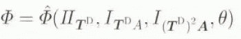
In this paper, we work with the constitutive form
for ϕ in the transverse isotropic case, where
represents the perpendicular to the isotropic plane in the material with unit normal a and θ the temperature. This isotropic plane in the material is that plane in which the material behaviour is independent of the loading direction, Requiring that Equation (3.2) satisfies material frame indifference, i.e. be independent of observer, Equation (3.2) reduces to
with I A = 1 and A 2 = A, where
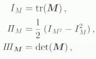
represent the invariants of some tensor M. It should be emphasized that it is the requirement that material behaviour be independent of observer that necessitates the introduction of the invariants. In addition to the usual invariants of T,
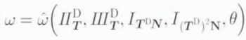
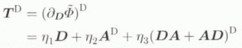
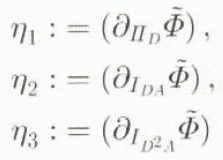
The relevance of working with the dissipation potential in the current context is the form
taken by D in terms of ϕ via Equation (3.1)2 and Equation (3.2), where
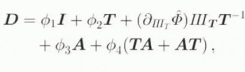
where

Note that
In this case, Equations (3.3) and (4.7) reduce to
and
respectively.
Assuming further as usual that the flow of ice is independent of pressure, i.e. p = –
where we have replaced T by its deviatoric part T D = T
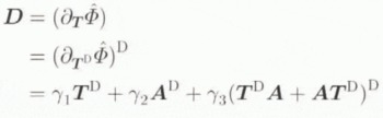
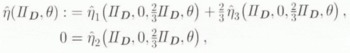
where now

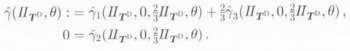
hold for the coefficients appearing in Equation (3.13). The reduced form of Equation (3.12) for the dissipation potential is that assumed by Van der Veen and Whillans (1990, appendix), whose approach is based on that of Johnson (1977). Note that γ2 must vanish as T goes to zero for D to vanish as well. In addition, note that Equation (3.13) is consistent with the incompressibility of ice, i.e. I D = 0 holds identically. Furthermore, Equation (3.13) reduces to a form equivalent to Glen’s flow law when, e.g. γ2 = 0 and γ3 = 0. As will be shown in what follows, however, there is another way that it can reduce to a form equivalent 10 Glen’s relation when A is allowed to evolve, i.e. when induced anisotropy is being modelled.
To understand the physical meaning of the material coefficients appearing in Equation (3.13), it is useful to examine this constitutive relation relative to an orthonormal basis (e 1, e 2, e 3), assuming at the same time, for example, that a is instantaneously parallel to e 3. In particular, then Equation (3.13) reduces to the matrix form
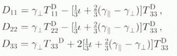
for the diagonal components, and
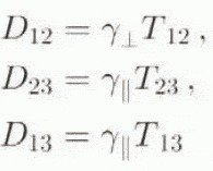
for the shear components, of D, with

From these component forms, we see that γ
4. Orientation Structure, Kinematics and Density
In any physical system consisting of a very large number of “structural” elements, it is generally impossible to model in detail the evolution of each element, as well as their interactions with each other. As such, tractable models for such systems are inevitably based on various kinds of idealizing assumptions. In particular, for polycrystalline materials consisting of perhaps many thousands, tens of thousands, or even millions, of crystals, one can idealize the corresponding evolving microscopic crystal texture macroscopically by assuming, analogous to superposed constituents in mixture theory, that a given (crystal) glide system exists in all orientations at each material point of the continuum.
Let r be the unit normal to these glide systems in the reference configuration, and n the corresponding unit normal in the current configuration, of the material. In the context of the multiplicative decomposition (Equation (2.1)) of the deformation gradient F, the elastic rotation R E determines the rotation of the crystal structure, and so the evolution of the glide-plane orientation, i.e.
The time derivative of this last relation yields the evolution relation
for n in the current context via Equations (2.2)2, (2.5) and (4.4), where
With W determined by the spatial variation of the spatial velocity field ẋ, the sole unknown quantity in Equation (4.2) is
(in the spirit of the “plastic spin” of Dafalias (1984)), with N = n ⊗ n where the coefficient
is in general an isotropic, scalar-valued function of T, N and θ; in accordance with the previous assumption that the flow of ice is independent of p, however, we have further assumed in writing Equation (4.5) thatω is independent of IT . In particular, note that the constitutive form of Equation (4.4) implies that the only non-zero components of

showing indeed that inelastic spin then takes place only in planes perpendicular to n.
Now, the major influence of the glide-plane orientation structure on macroscopic material behaviour is manifest in essence by the orientation distribution in the material. In the case of a continuum description of such a material, such a distribution can be described by an orientation-distribution function or orientation density f (e.g. Clement, 1982; Giessen, 1989), analogous for example to the classical mass density ϱ of the material. Distribution functions formally analogous to f can be found in kinetic gas theory, or the theory of liquid crystals with variable orientation (e.g., Blenk and others, 1991). Like the mass density, f depends on both time and space; unlike ϱ, however, f depends in addition on glide-plane orientation.
To formulate f heuristically, consider a finite distribution of N glide-plane orientations (e.g. a unit vector n and its negative − n) in the unit sphere S 2: = { n ϵ βͼ ͼ nͼ = 1} at some point x in the current configuration of the material body. Let the evolution of these N glide-plane orientations be described by the N time-dependent curves c i (t,x) (i = 1,. . ., N) in S 2. The distribution of such a discrete set of orientations at time t and position x can be represented in the form
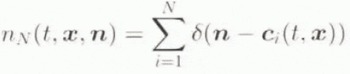
where δ is the Dirac delta function. Here, n N (t, x, n) represents the number of orientations in the distribution at time t and point x with unit normal n; further, since both n and − n lie on the perpendicular normal to the glide plane, nN (t, >x, n), = nN (t, x, −n), i.e. each orientation is described by both c i ,(t, x) and − c i (t, x). Integration of nN over S 2 results in the constant function
of t and x, where the integral has a value 2N since each orientation is counted twice, i.e. once for c i (t, x) and once for −c i ,(t, x) in the integration. Note that the integral of any continuous function φ on S 2 is given by
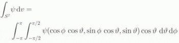
with x 1 = cos φ cos ̝. x 2 = sin φ cos ̝ and x 3 = sin ̝, where φϵ [−π, π] and ̝ϵ[−π/2, π/2,] are the “longitude” and “latitude” angles on S 2, such that n = cos φ cos ̝ e 1 + sin φ cos ̝ e 2 + sin ̝ e 3 in this chart. On the basis of Equation (4.7), the value of the time-dependent function
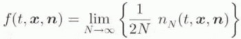
represents the number density of glide systems with unit normal n at time t and point x, and f(t, x, n) = f(t, x, −n). The definition in Equation (4.10) then yields the constant function
of t and x. Analogous to the total mass of a material body, the relation (4.11) implies that the total orientation of each material point is also conserved. As such, the evolution relation
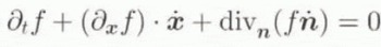
for f follows from Equation (4.11) via time differentiation and continuity of the integrand, where div n represents the divergence operator on S 2. The result in Equation (4.12) for the evolution of f is influenced by both that of the material as a whole, as well as that of the glide-plane orientations.
5. Example: Two-Dimensional Simple Shear
To look into Equation (4.12) in more detail, consider the special case of a two-dimensional polycrystalline material subject to a homogeneous simple shear (e.g. Giessen, 1989; Svendsen and Hutter, 1995). Since compression dominates in the upper, and shear in the lower, regions of natural ice masses, this example may be in particular relevant to the lower (basal) regions. In the two-dimensional case, the orientation structure evolves in S 1 (i.e. the circle) at each x, and the evolution relation (4.2) simplifies to
with n = −sin ̛ e 1 + cos ̛ e 2, where ̛ is the angle of the glide-plane orientation relative to the vertical (see Fig. 1). In the case of two-dimensional simple shear, we have the matrix form
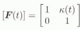
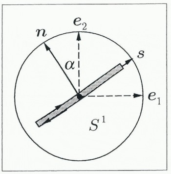
Fig. 1. Two-dimensional geometry of glide plane and its orientation in Sl
for the deformation gradient of the material relative to (e 1, e 2) (see Fig. 2), yielding the form
for Equation (5.1). To keep this example entirely kinematic, we can, rather than using Equation (4.4), assume for example that no instantaneous inelastic deformation of the glide planes takes place vertically. i.e.
with K(0) = 0. As an alternative kinematic constraint, we can assume that no instantaneous inelastic deformation takes place parallel to the glide planes, in which case n · L IS = 0 (see Fig. 1), implying
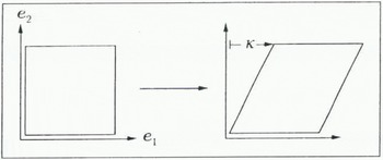
Fig. 2. Time-dependent simple shear of the material in the e1 direction by the amount k(t)
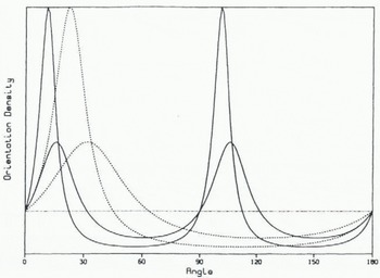
Fig. 3. Relative orientation density as a function of α for two values of K. The smaller and larger solid curves represent Equation (5.8) for K = 0.5 and K = 1, respectively. Likewise, the smaller and larger dashed curves represent Equation (5.7) for K = 1 and K = 2, respectively. The dotted straight line represents a uniform distribution. The vertical scale is irrelevant.
yielding
which appears similar to Equation (5.4) hut in fact leads to different maxima for f, as we next show. Assuming next that f is independent of x in this example,Equation (4.12)reduces to
where now f is a function of t and α. In the context of Equation (5.4), this last result can he integrated to yield the form
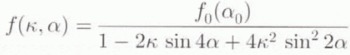
for f (replacing t by K) when no instantaneous vertical inelastic deformation in the glide planes takes place, where f 0 is the initial distribution of glide-plane orientations. On the other hand, integration of Equation 5.6) using Equation 5.5) leads to the form
for f when no instantaneous inelastic deformation in the glide planes parallel to these takes place.
The results in Equations (5.8) and (8.7) ran be compared qualitatively with observations on the emergence of an oriented texture in natural ice. Assuming the initial distribution f 0 is uniform, i.e. f 0 = 1 /2π on S 1, the result Equation (5.8) is displayed in Figure 3 as a function of oriention α for various values of the amount of shear K. As shown in tins figure, Equation (5.8) implies a bimodal distribution for the glide-plane orientations which tend towards the vertical and horizontal with increasing shear, while Equation yields a single-maximum density of glide-plane orientations tending towards the vertical with increasing shear. In the latter case, this tendency is certainly due mainly to the constraint
6. Texture Evolution and Material Behaviour
In the current model, we assume that the large-scale alignment of the caxes, and so basal slip planes, in the hexagonal ice crystals leads to a iransverse-isotropic material behaviour, with the transverse isotropic plane in the material at a given point corresponding to the “mean” glide plane there. As such, we are interested in the orientation of this mean glide plane, representing simultaneously that of the transverse isotropic plane of the material by constitutive assumption. This “macroscopic” orientation is given in fact by the second moment
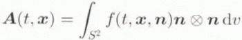
of the orientation-distribution function integrated over S 2, a constitutive assumption that is consistent with the definition of A as given in Equation (3.3) in the sense that
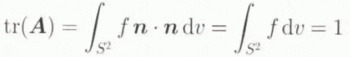
follows from Equation (4.11). The constitutive relation (6.1) clearly connects the evolution of the glide-plane orientation distribution f as determined by Equation (4.12) to the macroscopic material behaviour as given by Equation (3.13).
The relevance of the constitutive assumption (6.1) for A in terms of the evolution of the glide-plane orientation (micro)structure can be appreciated for example in the context of the special case of a uniform (i.e. random) distribution of crystal glide-plane orientations at each material point, in which case

holds with ʃ S 2 dʋ = 4π. In this case. A reduces to
from Equation (6.3). For a uniform f, then, we obtain
i.e. the form of Glen’s flow relation, with
As such, a random distribution of crystals in the material leads to macroscopic isotropic material behaviour in the current model, as would be expected physically. Note that the result in Equation (6.6)2 is consistent with the assumed form for γ2 in Equation (3.17)3 above.
7. Discussion
The ultimate goal we have in mind for the induced anisotropy model formulated in this work is of course to incorporate it into a numerical simulation of the motion of large ice masses, something that is not feasible with Talyor–Bishop–Hill-type models for such anisotropy (e.g. Van der Veen and Whillans, 1994). Since this represents work in progress, however, we finish up with a brief discussion of some of the aspects of this implementation which are currently being worked out.
As is well known, the basis of any such numerical simulation of the evolution of a glacier or ice sheet is the usual balance relations for mass, momentum and energy, which in this context take the particular forms
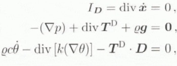
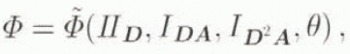
respectively, where
for the dissipation potential, whose material frame in different form reduces to
when we assume that ice is incompressible (i.e. ID = 0), and note that D is not invertible (since it can be zero), requiring
for the deviatoric part of T, where
define the coefficients in Equation (7.4). In particular, when f is uniform, A D = 0 follows from Equation (6.4), and so
with
analogous to Equation (6.6). Clearly, Equation (7.6) can be rewritten in the form of Glen’s flow relation since η ≠ 0. Indeed, comparing Equations (6.7) and (5.6), we have η = σ−1.
With T D determined in general by Equation (7.4), the only remaining field at the macroscopic level to be specified is A. The spatio-temporal evolution of A as determined by Equation (6.1) is based on that of f as given in Equation (4.12), which in turn depends on the spatial velocity ẋ of the body, as well as the evolution of n given by Equation (4.2). This latter evolution is determined by the body spin W (and so the initial conditions) as well as the constitutive relation (4.4) for
where now
analogous to Equation (4.27). In conclusion, then, Equations (4.2), (4.12), (6.1), (7.4) and (7.8), together with the balance relations (7.1), represent a closed system of equations for which initial boundary-value problems can be formulated and solved, once functional forms for the constitutive quantities с, K, η1, η2, η3, and ν, are established, the latter four being functions of II D , IDN , ID2N and θ. A first step in this direction currently under investigation is to assume с and K are unaffected by the induced anisotropy, i.e. use the standard constitutive forms for these, and concentrate on the forms of the remaining material properties. To this end, note for example that the result in Equation (7.7)2 suggests that η2 could be proportional to (a power of) IDN . On this basis, we are currently investigating power-law type relations for all four of these material coefficients analogous to that in Glen’s flow relation satisfying the asymptotic relations (7.7) in the case of isotropy.


