


Introduction
Surface measurements of glacier movement have occasionally revealed significant changes of horizontal velocity within short periods of time, a few days or even a few hours (e.g. Reference IkenIken, [1978]). More recent short-term measurements included vertical velocity which showed related variations. The dependency of the velocity variations on melt- or rain-water supply suggested that the variations were caused by changes in subglacial water pressure. In particular the substantial variations of vertical velocity observed in a detailed study have been interpreted as variations of water storage at the bed. Footnote * A mechanism explaining the typical features of the observations is now sought. The following water-pressure-dependent sliding mechanisms have been proposed in the past:
-
Sliding over a lubricated, undulating, or three-dimensionally rough bed with formation of water-filled cavities (Reference LliboutryLliboutry, 1968, Reference Lliboutry1979; Reference KambKamb, 1970).
-
Change of thickness of the lubricating water film between ice and bedrock (Reference WeertmanWeertman, 1962).
-
Deformation of saturated sediments below a glacier (Reference BoultonBoulton, 1979; Reference JonesJones, 1979).
-
Participation of subsole drift in the sliding process (Reference Engelhardt, Engelhardt, Harrison and KambEngelhardt and others, 1978; Reference Kamb, Kamb, Engelhardt and HarrisonKamb and others, 1979; Reference Boulton, Boulton, Morris, Armstrong and ThomasBoulton and others, 1979).
-
Slip along water-activated shear planes within a glacier (Reference TyulinaTyulina, 1976).
If the velocity variations are indeed caused by short-term water-pressure variations which are synchronous over large areas of the glacier bed, then high permeability of the subglacial drainage system is an essential assumption. This requirement is best satisfied if bed separation is extensive. Extensive bed separation also provides an appropriate explanation for the variations of vertical velocity which may then be understood as the result of simultaneous growth (or shrinkage) of subglacial, communicating cavities. It thus appears probable that the velocity variations in the quoted field examples were a direct consequence of sliding over an undulating bed with bed separation controlled by a varying subglacial water pressure. Certainly, other mechanisms may have played a part; in particular, friction between rock particles in the ice sole and below has probably modified the observed variations of the sliding velocity. The present paper will be confined, however, to an understanding of the principles. It concentrates on the idealized problem of sliding on a perfectly lubricated bed with the action of an imposed water pressure. To a large part this problem is well known, owing to the comprehensive sliding theories of Reference KambKamb (1970) and Reference LliboutryLliboutry (1968, Reference Lliboutry1979). The pioneering ideas on the action of the subglacial water pressure were developed in the original work of Lliboutry, yet the transient stages of cavity growth and shrinkage have not been analysed so far. It is exactly these phases, however, which seem to determine the velocity variations in question.
Fundamental considerations of the effect of the subglacial water pressure acting on a glacier sole with non-uniform pressure distribution
In the absence of a basal shear stress the pressure which the ice exerts on its bed is every-where p 0, the ice overburden pressure. If, however, the basal shear stress is not zero, the pressure on the bed is no longer uniform, but is larger than p 0 on the stoss faces of bedrock protuberances and smaller on the lee faces, so that equilibrium of forces is maintained. It is in the low-pressure zones at the lee faces where a change of water pressure caused by, say, a change of water input into the subglacial drainage system can affect motion of the glacier even if the water pressure stays well below the ice overburden pressure. The lower bound of water pressure which has an effect is the minimum pressure occurring at the lee faces, the separation pressure. At a larger water pressure a part of the ice sole is separated from the bed. The separation pressure has been introduced and given in quantitative terms in the sliding theories of Reference LliboutryLliboutry (1968), Reference NyeNye (1969), Reference KambKamb (1970), Reference MorlandMorland (1976), and others. For the special case of a sinusoidal bed the separation pressure p s is

where τ is the basal shear stress, λ the wavelength, and α the amplitude (one half of the difference of the maximum and minimum of the sine function).
Another important parameter is the limiting water pressure above which the sliding becomes unstable, that is to say, a non-zero acceleration term enters into the balance of forces. This pressure is well below the ice overburden pressure. C. F. Raymond and H. Röthlisberger (personal communications) have independently arrived at the prediction of this pressure and have derived an explicit expression.
A simple derivation is as follows: Consider a plane-parallel slab of thickness d and of large lateral extent resting on a lubricated, undulating bed with a mean slope α. For a moment we will assume a particularly simple shape of the bed: a bed consisting of rectangular steps (Fig. 1). An ice column of unit width and length l rests on the faces b and c of the steps, its weight is F 1 = pgdl. The component perpendicular to face b is
and the component perpendicular to face c is
where ρ is the density of the (ice) slab, g the acceleration due to gravity, β the angle which the stoss faces make with the down-slope direction x (Fig. 1), and β—α the angle between the stoss faces and the horizontal, i.e. the backward inclination of the steps.

Fig. 1. Diagram illustrating the derivation of the limiting water pressure of stability. An ice slab of thickness d is resting on a stepped bed with a mean slope ∝.
The corresponding mean pressures on faces b and c are

and

Thus, if a water pressure p W > p c opposes p c there will be a net force on the ice which will move it upward along faces b with accelerating velocity. The limiting pressure p c will in the following be designated p 1.
Equivalent expression for p 1 are:

The ice overburden pressure is p 0 = pgd cos α. and τ = pgd sin α is the basal shear stress. The last expression in Equation (2) is also appropriate if the basal shear stress is given by the more general expression τ = fρgd sin α where f is a shape factor taking into account the drag of the valley sides. The validity of Equation (2) is not restricted to a bed consisting of rectangular steps; the equations hold for other two-dimensional bed undulations as well if the steepest tangents on the stoss faces make an angle β with the mean bed slope. This is readily seen if one assumes that the spaces between the stepped bed and another bed, for example the one which is sketched on the right of Figure 1, are filled with a weightless liquid. Inserting the liquid does not affect the balance of forces and the pressure is constant over the surface of the liquid. Further, the equations apply also to three-dimensionally rough beds if the projection of the total area exposed to the water pressure on a plane which is normal to the direction β is the same as in the two-dimensional case.
For the special case of a sinusoidal bed the steepest tangent of the stoss face is
and thus
In the formulation of the overall force balance the material properties of the glacier are irrelevant. However, there are differences in the pressure distribution and size of contact areas when the glacier is assumed to be viscous rather than rigid. When the water pressure rises to the limiting value, a rigid body on an undulating (e.g. sinusoidal) bed is in contact with the bed only at the inflexion points of the stoss faces. A viscous body, however, touches the bed on finite areas so that extreme stress concentrations are avoided. Consequences of this difference will not be pursued further in this paper.
A stability limit for sliding under the action of a water pressure has already been derived by Lliboutry in a different way. For the case of a sinusoidal bed he has found a maximum, limiting value of the reduced friction f
W/f
0 of 1.325 (Reference LliboutryLliboutry, 1968, p. 34). This value refers to a maximum size of stable cavities, they cover one-half of the sinusoidal bed. By definition f
w = τ and  , hence Lliboutry’s limiting value of the water pressure is
This value is smaller than that derived above (Equation (3)). The difference may result from Lliboutry’s assumption of a symmetric pressure distribution on a (large) contact area, which has its centre well above the inflexion point of the stoss face (Reference LliboutryLliboutry, 1968, p. 33).
The remaining part of this paper deals with water pressures below the limiting pressure which correspond to the stable range of sliding velocities. Before discussion of the numerical analysis, the effect of a water pressure which is in the range between the separation pressure and the limiting water pressure will be described in a qualitative manner.
When water at the pressure p W in this range penetrates to the lee faces of the protuberances of the glacier bed, a part of the ice sole is subjected to the boundary pressure p W and is thus separated immediately from the bed, a separation which includes not only that part where the normal stress had originally been smaller than p W but a larger zone as a result of a cantilever effect. In the subsequent process of cavity growth, the ice in the central part of the separated zone no longer moves parallel to the bed but away from it. The lower edge of the separated zone moves further along the bed while the upper edge retreats only a little from its original position. Thus, the extent of that part of the ice sole which is supported by water at the pressure p W becomes much larger in the course of time. When the cavity has grown to its final, steady form the ice at the ceiling moves parallel to it.
Assumptions for the Numerical Model
The present analysis is based on several assumptions:
-
1. No tangential stresses at the ice–bed interface.
-
2. A linear flow law for the ice. The ice is taken to be nearly incompressible in time; more specifically, that parameter which is the linear viscous analogue of Poisson’s ratio in elasticity is assigned the numerical value 0.499. Perfect incompressibility in time would require the numerical value 0.5, which is not acceptable for the finite-element program.
-
3. Plane-strain, periodic bed undulations in the xz plane.
-
4. Instant supply or drainage of water of a given pressure at all lee faces of the undulating bed.
-
5. No regelation.
Geometry of the Model
The finite-element analysis was applied to a section representing in two dimensions a small part of a glacier at its base. This section (Fig. 2) was taken to be 25 m high and 60 m long. It is resting on an undulating bed which has a mean slope of 4°. The wavelength of the undulations was chosen to be 20 m, the amplitude 1.5 m. This section is part of an infinitely-wide ice mass which is 310 m thick (measured vertically in space) and has a surface- and bed-slope of 4°. Thickness and slope are the same as at the central part of the Unteraargletscher where series of short-term movement measurements have been made.
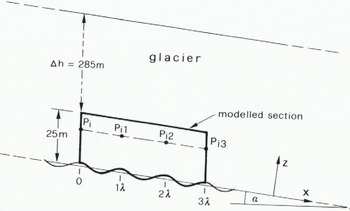
Fig. 2. Modelled section at the bottom of a glacier. Surface slope and mean bed slope of the glacier is ∝ = 4°. Bed undulations have a period of λ= 20 m.
Method of Numerical Analysis
The calculations were carried out with the finite-element program STAUB. This computer program and a related plotting program were developed at the Institut für Strassen-, Fels-, und Eisenbahnbau, Eidgenössische Technische Hochschule, Zürich, for the purpose of stress and strain analysis in tunnel construction work (Reference Kovári, Kovári, Hagedorn, Fritz and DesaiKovári and others, 1976). Different program versions for elastic and plastic materials and for substances with composite properties exist. For the present purpose the elastic version (Reference KováriKovári, 1969) has been used; this is equally applicable to the analysis of a Newtonian liquid because there is a complete analogy between the elastic stress-strain relations and the linear viscous stress-strain-rate relations. In this application the shear modulus is replaced by a viscosity which was arbitrarily assumed to be η = 2.273 × 10¹³ Pa s (= 7.208 bar a). This particular assumption does not affect the calculated stress field, but only the scale of the velocity vectors.
Boundary Conditions
(a) Lower boundary
The ice at point P i on the ice-rock interface moves parallel to the interface; in the finite-element approximation this direction was specified to be parallel to the line connecting the two neighbouring nodal points Pi−1, and P i+1 on the interface. (Vice versa, the movement of a nodal point, calculated by the program, was considered to be parallel to the interface, if the same condition was satisfied.)
Where the ice sole was supported by water of a given pressure, the corresponding force per unit width at a nodal point P i was calculated as
Here p wi is the water pressure at the depth of the point P i and b i is the distance between two neighbouring nodal points P i−1 and P i+1 on the interface. Because of the cantilever effect mentioned above, the extent of the area on which a given water pressure can act is not known exactly at the beginning. Therefore, after running the program, it was necessary to make sure that the points on the edges of the separated zone did not move downward into the bed but parallel to the interface or upward. On the other hand, the pressure calculated by the program for a point remaining on the assumed ice-rock interface ought to be larger than the given water pressure; if this was not the case the extent of the ice-water interface was changed and the program was run again.
(b) Upper boundary
Normal stress p S and shear stress τ S on the upper boundary result from the weight of the ice layer on top of the modelled section. In a real glacier the drag of the valley sides reduces the shear stress. In order to account approximately for this reduction a shape factor f = 0.5 has been assumed in the calculation of τ s.
Thus
and
where ∆h = 285 m and α = 4° (see Fig. 2). ρ is the density of the ice and g the acceleration due to gravity.
Components of the force acting at a nodal point P i on the upper boundary are

where b i is the distance between the two neighbouring points P i−1 and P i+1 on the boundary.
(c) Sides of the modelled section
Since the stresses vary in a non-linear way along the sides of the section, the force components in a nodal P i were calculated from the stresses at the three successive points P i−1, P i, and P i+1 on the boundary according to an interpolation formula commonly used in statics. The stresses on the lateral faces were, however, not known at the beginning and had to be determined by means of an iteration. In the first step these stresses were tentatively assumed to be equal to those on a vertical cut in a plane-parallel inclined slab of ice which is frozen to the bed. On this assumption, stresses in the interior of the modelled section were computed, from which the boundary stresses for the second iteration step were deduced as follows: Consider a line parallel to the x-axis which is drawn through a nodal point P i on the left side of the section. The points on this line at distances λ, 2λ, and 3λ from P i are labelled P i1, P i2, and P i3. The arithmetic mean of the stresses in P i1 and P i2 was assigned to the boundary point P i. The same mean stresses but with opposite sign were allocated to the boundary point P i3 If the iteration were continued entirely in this way a possible superimposed longitudinal stress could not be eliminated. Therefore the arithmetic mean of computed velocities in P i1 and P i2 was prescribed at P i (and P i3 ) in every second step. The iteration was continued until the velocity did not vary along the upper boundary by more than 3.5%.
A Problem in Modelling Water-Filled Cavities
Let nodal points situated on the bedrock profile be labelled P 1, P 2, P 3, .... Points on the ceiling of a cavity are marked with a star. The point P i (≡ P i *) at the corner of a cavity (Fig. 3) is in contact with the bed and should move parallel to the original bed, that is parallel to the line connecting P i−1, and P i+1. In accordance with the specification given above, however, the point moves parallel to the line connecting the points P i−1 * and P i+1. (Disregard of the specification would imply that forces act on a surface which is not closed.) Calculations carried out for various positions of point P i−1 * showed that the overall sliding velocity depends nearly linearly on the direction of movement of the point P i. The dependency is negligible for small cavities but very strong for large ones. For example, in the case of the largest cavity modelled (Fig. 6b) a variation of the direction of movement of point P i by 1° caused a change of the sliding velocity by 16% at a water pressure close to the steady-state value. The difficulty is avoided to a large extent by putting P i - 1 * approximately on the bedrock surface at a very small distance from P i. A change of the distance between P i - 1 * and P i affects the sliding velocity very little. In the case already quoted, an increase of this distance by 33% caused a change of the sliding velocity by 1.2% only. Some uncertainty, however, remains. Indeed, not even the “slope of the original bed” is well defined in the finite-element approximation if distances of nodal points are varied. The tolerances shown in the final plot of sliding velocities (Fig. 8) refer to the uncertainty.

Fig. 3. Finite-element approximation of a water-filled cavity. The nodal point Pi marks the edge of the cavity.
Modelling of Steady Cavities
These are cavities which are neither shrinking nor expanding at the given water pressure; at the cavity ceiling the ice moves parallel to it, the sliding velocity does not change with time as long as the water pressure is constant.
The appropriate cavity geometry was found by a trial-and-error approach, an arbitrary shape was assumed at first. Running the finite-element program with boundary conditions corresponding to this cavity shape revealed that a cavity was shrinking in some places and expanding in others. Accordingly, nodal points of the cavity ceiling were put into slightly different positions in the next iteration (e.g. the cavity was made wider where it had been expanding). This procedure was continued until nodal points of the cavity ceiling moved (approximately) parallel to the ceiling.
Results of the Numerical Modelling
List of numerical values to which results refer

The flow on a nearly sinusoidal bed was modelled as a reference. Then the shape of the lee faces was modified while the shape of the stoss faces and the periodicity were held unchanged in all cases studied. The velocity fields on the nearly sinusoidal bed and on a bed with steeper lee faces are shown in Figure 4b and a. Figures 5a to 6b illustrate the effect of water pressure p W = 24.1 bar. In Figure 5a and b the stage at which cavity growth begins on the beds of Figure 4a and b is shown. Figure 6a represents the sliding over water-filled cavities which have almost grown to their steady size, in Figure 6b larger cavities are shrinking at the given water pressure. Their shape was derived for steady conditions with the water pressure at 24.4 bar. In Figure 7 the water pressure is reduced to 23.6 bar; the cavities are the same as in Figure 6a. This small pressure drop causes the ice initially to slide backwards.

Fig. 4. Velocity field in Newtonian liquid on a perfectly lubricated bed with periodic undulations, a. Bed with steep lee faces; b. nearly sinusoidal bed. The scale of the velocity vectors refers to a viscosity η = 2.273 × 10¹³ Pa s ( = 7.208 bar a).

Fig. 5. A water pressure of 24.1 bar = 246 t/m2 (arbitrary pressure in the stable range) acts on the lee faces of the beds shown in Figures 4a and b. Shading indicates the separated zone. The dotted line traces a flow line.

Fig. 6. Water-filled cavity. a. Approximately steady at the pressure of 24.1 bar; b. shrinking at 24.1 bar. This cavity is steady at a water pressure of approximately 24.4 bar. The dotted lines trace flow lines.

Fig. 7. The same cavity as in Figure 6a, but with a water pressure of 23.6 bar = 241 t/m2.
The actual sliding velocity had to be derived in an additional computation from the velocity at a sufficient height above the bed, in the present case the velocity on top of the modelled section was used. From this velocity the proportion due to internal shear in the ice below was subtracted. The sliding velocity obtained in this way for the nearly sinusoidal bed is 12% less than the theoretical value deduced for an exactly sinusoidal bed (e.g. Reference NyeNye, 1969). The main reason for this disagreement appears to be that the modelled undulations have a relatively large roughness a/λ while the quoted theory is strictly valid for beds with small roughness only. The present result agrees well with a theoretical prediction by Raymond, which allows for the actual roughness (C. F. Raymond, personal communication).
In Figure 8 the x-components of sliding velocities are plotted against water pressure for the different shapes of lee faces considered in the models: Curve I refers to the geometry of Figure 4a, Curve II refers to the nearly sinusoidal bed (Fig. 4b), lines III and IV represent sliding with the cavities shown on Figure 6a and b. The horizontal branch III depicts the sliding velocity when the cavity ceiling in Figure 6a is replaced by bedrock. The dotted line gives the steady-state sliding velocities; i.e. the sliding velocities when steady cavities have formed. Below this line cavities are shrinking.

Fig. 8. Plot of sliding velocity versus water pressure. u is the x-component of the sliding velocity; the index s refers to (steady-state) sliding on the sinusoidal bed at the separation pressure. u/us is the x-component of the sliding velocity expressed as a fraction of the sliding velocity on the sinusoidal bed at the separation pressure. p1 is the limiting water pressure at which sliding becomes unstable. Curves I to IV show the initial, transient sliding velocity at the instant when the water pressure is applied (except for the horizontal parts and two points on lines III and IV which show steady-state sliding). Curve I refers to sliding on the bed shown in Figure 4a, curve II refers to the sinusoidal bed, lines III and IV refer to sliding with the water-filled cavities of Figures 6a and b, respectively. The horizontal branch III depicts the sliding velocity when the cavity ceiling in Figure 6a is replaced by bedrock. The dotted line marks steady-state sliding, below this line cavities are shrinking (indicated by broken lines).
From the examples in Figures 4 to 7 and from the diagram in Figure 8 the following trends are apparent:
The smoother the ice-sole profile, the larger the sliding velocity (the velocity increases in the sequence of Figures 3a, 3b, and 6a). This is what one would expect.
When a given water pressure is applied, the resulting increase in the sliding velocity is the larger, the steeper the ice sole at the lee side of humps or, more specifically, the smaller the separation pressure of the particular bed. Indeed, not only is the velocity increase larger when the ice sole at the lee faces is steeper, but also the absolute magnitude of the sliding velocity becomes larger provided that the water pressure is sufficiently large. This effect would be much more marked if actual roches moutonnées were considered rather than the modelled smooth glacier beds. (Of course, when the water pressure becomes so large that spontaneous separation reaches a point on the common stoss face, the differences between the sliding velocities on beds with different lee faces disappear.)
The response of the sliding velocity to a change of water pressure is the more sensitive the larger the area of the ice sole which is subjected to the imposed water pressure. This is evident from the slopes of the velocity-pressure curves in Figure 8. A closer inspection, however, shows that it is not simply the size of the area subjected to the water pressure which determines the slope of the velocity-pressure function, but the orientation of this area is also influential.
The sliding velocity varies linearly with the water pressure as long as the area of the ice sole which is subjected to the imposed water pressure is constant. The relationship is of the form
where u(p W) is the transient sliding velocity at a water pressure p W, u St is the steady-state sliding velocity for the given cavity size, p St is the water pressure at which the considered cavity is steady, and C is a constant which depends on size and orientation of the area covered by the cavity and on the geometry of the remaining contact area. Numerical values of Care: 64 for line III (Fig. 8) and 51 for line IV.
In the finite-element model the area of spontaneous separation of the ice sole increases in finite steps with increasing water pressure, therefore curves I and II consist of finite sections of straight lines. Once cavities have formed, a further increase of water pressure does not cause an additional spontaneous separation, but only slow cavity growth—as long as the pressure increase is not very large. Therefore, the sliding velocity is approximately given by Equation (5) during a finite period of time.
Discussion
Considering the effect of a water pressure p W, acting on the ice sole at the lee sides of bedrock obstacles, different phases have been distinguished:
-
(1) transient phases
-
(a) instantaneous separation, which is in our terminology the instantaneous re-distribution of pressure by the action of the water pressure p W ;
-
(b) various stages of growing or shrinking cavities;
-
-
(2) steady-state sliding over cavities which are steady at the given water pressure.
First a remark is due concerning the extent and effect of instantaneous separation. It has already been mentioned that the separated zone is larger than that part of the ice sole which had originally been subjected to a normal pressure
p
W. In other words, when separation takes place, the pressure on the central, steep part of the separated ice sole is increased while it is decreased along the edges of the separated zone. At first sight it may therefore appear that no net force change at the lee faces is accomplished by the action of the water. This is, however, not so since the separated zone is curved. Therefore, at the instant of separation, the positive and negative pressure changes at the ice sole correspond to force changes which do not compensate. Indeed, the action of the water pressure causes a net increase of the force exerted on the ice in the x-direction, in contrast to a slight decrease in the z-direction. The increase of force in the x-direction causes an equivalent increase of pressure on the stoss face. This effect could also have been caused by an increase of the basal shear stress. In either case the sliding velocity increases—linearly with the driving force when the flow law is linear.
It has been seen that the effect of a water pressure p W on the sliding velocity is largest at the instant of separation and then gradually decreases until steady cavities have formed. It is informative to compare the distribution of forces on the ice sole in the different cases; for illustration a particularly simplified bed will be considered. In Figure 9a the mean normal stress on face a2 and on face a4 is equal to p 0, the ice overburden pressure. The mean normal stresses on faces a1, and a3 are p 1 = p 0 — ∆p and p 3 = p 0 + ∆p, respectively, where the magnitude of ∆p depends on the basal shear stress. If a water pressure p W > p 1 separates the ice from the faces a1 and exerts an additional force on the ice sole, the stress on a3 increases to p 3 ’ = (p W – p 1) + p 3. Figure 9c shows the situation when cavities have grown under the influence of the water pressure p w. The mean stress on faces a3 is still p 3’. The stress on a2, however, is reduced to p w while the stress on a4 is increased to p 4” = (p 0 a 4 + (p 0–p w)a 2)/a 4. It is only this re-distribution of pressure on troughs and crests which causes the differences in sliding velocity at the beginning of cavity growth and when steady cavities have formed. The larger pressure in the wave troughs during the phase of cavity growth permits flow along straighter flow lines, i.e. a nearly rigid movement of a part of the basal ice. Therefore the sliding velocity is larger than in the steady-state. This is generally valid and illustrated in Figures 5 and 6.

Fig. 9. Typical stress distributions, illustrated with simplified glacier bed. a. Stress distribution before water at a given pressure pW has access to the lee faces; b. a water pressure pW > p1 acts on the lee faces; c. cavities have formed.
The present results have been obtained on the basis of very simplistic assumptions. More realistic assumptions would change the results in the following ways:
-
The introduction of a tangential stress at the ice-bed contact, for instance a Coulomb friction law, has an effect similar to that of a reduction of the basal shear stress. Both the separation pressure (Equation (1)) and the limiting water pressure (Equation (3)) attain larger values. The difference in sliding velocities at the commencement of cavity growth and with steady cavities is reduced since in the latter case the contact area is smaller and so is the friction.
-
If the linear flow law is replaced by Glen’s law the difference between the transient and steady-state sliding velocity becomes larger presumably, because, when cavities begin to grow, ice deformation is more strongly concentrated in zones at the stoss faces than it would be in the steady-state giving a particularly small effective viscosity there of η e = ½A n /τ e n−1 Here τ e = (σ ij' σ ij'/2)½ is the effective shear stress and A and n are constants in Glen’s flow law:
 = τ
e
n−1σ
ij'/An
. Furthermore, the straight lines in Figure 8 are replaced by parabolas.
= τ
e
n−1σ
ij'/An
. Furthermore, the straight lines in Figure 8 are replaced by parabolas. -
If, instead of periodic bed undulations, geometrically similar undulations with different wavelengths are assumed, the basal shear stress is no longer uniformly distributed amongst the different wavelengths; in order to maintain a uniform sliding velocity the smaller undulations require a larger proportion of the mean basal shear stress. Therefore, separation starts at the smaller obstacles at a smaller water pressure. Nevertheless, instability is attained no sooner than when the water pressure rises to the same limiting water pressure as in the case of periodic bed undulations. If the stoss faces of bed undulations have different maximum slopes, a rigid-body translation is only possible in the direction of the steepest stoss face which therefore determines the limiting water pressure for stability. Of course, if steep stoss faces are few, stress concentrations are immense when the limiting water pressure is approached. Consequently sliding is very fast and ice fracturing may occur.
-
In reality, not all low-pressure zones at lee faces are in communication with subglacial drainage channels as has been assumed. For this reason the computed effect of the subglacial water pressure is an upper bound to the true effect which depends strongly on the degree of branching of the subglacial drainage system of a particular glacier in a certain season. Furthermore, the capacity of water flow towards the low-pressure zones is not unrestricted. If the water pressure rises to the limiting pressure the sliding velocity is limited by the rate of water input into the subglacial cavity network.
-
The contribution of regelation sliding to the total sliding velocity is negligible for the size of undulations modelled. However, the possibility that freezing of the ice sole occurs in zones where the pressure is temporarily reduced as a consequence of water-pressure variations cannot be dismissed. This mechanism has been discussed by Reference RobinRobin (1976). It is beyond the scope of the present paper to investigate its effect on the variations of the sliding velocity in more detail. It is noted, however, that some field observations indicate that the freezing mechanism is not influential enough to obscure variations of the sliding velocity which are consistent with the present model. The largest temporary pressure reduction takes place at the crests of bedrock obstacles at the time of rising water pressure in the cavities. One would therefore expect the most extensive refreezing of the ice sole to the bed (and consequently a small sliding velocity) in this time. Measured sliding velocities, however, were largest during the time of maximum or rising water pressure in moulins (Reference IkenIken, 1974, pp. 90, 94, and 96).
Conclusions
The study of the idealized model has made characteristic features of the relation of subglacial water pressure and sliding velocity distinct. The sliding velocity is neither simply a function of the subglacial water pressure nor of the size of cavities but depends on both variables. The result that the largest sliding velocity (in the stable range) occurs at the beginning of cavity growth and not when the steady-state size of cavitation is attained may correspond to the field observation that the maximum horizontal velocity occurs before the upward motion of the ice has reached the maximum elevation.* Backward sliding, predicted by the model for the case of rapidly shrinking cavities, has not yet been observed. It would be an indication of the significance of the cavitation mechanism. For this test short-term velocity measurements ought to be continued during the night. Depending on the type of glacier and subglacial drainage system it may, however, happen that the channels which interconnect the cavities become blocked, when the water pressure drops and thus the shrinking process is stopped.
Of particular interest is the possibility of unstable sliding at a water pressure well below the ice overburden pressure. The very high velocities observed during brief periods at the beginning of the melt season may possibly be interpreted as short spells of locally unstable sliding, terminated by the loss of water from the subglacial system.
Acknowledgements
This study has gained much from the discussions with C. F. Raymond and H. Röthlisberger who took a particular interest in the problem and helped to clarify the concepts. They also read the manuscript and suggested improvements. U. Spring, K. Hutter, and G. Raggio also participated in some of the discussions. P. Fritz of the Institut für Strassen-, Fels-, und Eisenbahnbau of Eidg. Technische Hochschule (ISETH) advised on the use of the finite-element program STAUB. The drawings were prepared by B. Nedela and S. Dimmler typed the manuscript.


