Selected aspects of borehole completion

Figure 2 shows the timeline of scientific operations following borehole completion on 27 January 2013, at ~8 PM local time (all times are given here in coordinated universal time (UTC) +12 h). Although drilling operations are not the focus here, we discuss some aspects that are particularly relevant to scientific measurements and sample collection.

The WISSARD hot-water drill made a connection to the base of the ice sheet at 8:04 AM on 27 January 2013. About an hour before the anticipated breakthrough, water level in the borehole was pumped down to ~110m below ice surface to make sure that borehole water pressure was lower than SLW water pressure. The flotation pressure was calculated to be equivalent to borehole water level at -80 m below surface, based on the best estimate of ice thickness of 802 ± 10 m, from active-source seismic data (Reference HorganHorgan and others, 2012). An independent estimate of ice thickness from ground-based radar surveys yielded 797±10m (Reference Christianson, Jacobel, Horgan, Anandakrishnan and AlleyChristianson and others, 2012). The flotation level was calculated from ice thickness following the approach of Reference Engelhardt and KambEngelhardt and Kamb (1997).

Recordings from a water-pressure transducer installed near the return water pump show that, at the time of the breakthrough, water rose within <1 min by 28 m. The transducer output was recorded by the drill control software at 1 min intervals, but the real-time visual output to the command center display took place at 1 s intervals. The drill operator at the time noted that the main phase of borehole water-level adjustment occurred in just 2 s. This rapid equilibration contrasts with minutes-long breakthroughs observed by Reference Engelhardt and KambEngelhardt and Kamb (1997) in boreholes drilled on various Siple Coast ice streams.

If the borehole is assumed to have a simple cylindrical shape with the design radius of 0.3 m then ~8m³ of lake water rushed into the borehole from the subglacial environment during breakthrough. However, the volume of the upper part of the borehole, which determines how much water must enter to equilibrate water pressure to the flotation level, was likely larger than a simple cylinder because a parallel but interconnected return pump borehole was drilled right next to the main SLW hole. At the point of breakthrough, the drill nozzle flow was at a low level of just less than 1 L min^–1. It was lowered from its normal level of ~115 L min^–1 at 7:20 AM in anticipation of the breakthrough. Seven minutes after breakthrough the drill flow rate was increased to 135 L min–¹, and the process of borehole reaming back to the top lasted until 7:40 PM.

Borehole camera

Following its completion, the SLW borehole was visually inspected to determine if it could be used to deploy our scientific equipment. We used a borehole camera, which is part of the Micro-Submersible Lake Exploration Device (MSLED) (MS1 in Fig. 2). It consists of a cylindrical pressure housing with lights around its rim and a down-looking Go-Pro Hero 3 camera sending video to the surface through a Kevlar-reinforced fiber-optic cable with length markings. The camera enabled real-time visual inspection of the SLW borehole and subglacial cavity (Fig. 3).

Fig. 3. Image of sediments at the bottom of SLW obtained by the MSLED camera. The top of the sedimentary layer crumbled as the camera housing touched it. The view shown here is nearly vertically down and the housing window is ~0.3 m in diameter.

Conductivity-temperature-depth (CTD) profiler

After visual assessment of borehole quality, we deployed a CTD profiler, Sea-Bird SBE 19 plus V2. We used conductivity and temperature data to calculate water salinity based on the equation of state for water (EOS-80, Sea-Bird Electronics, 2013) (Fig. 4). For low-salinity waters, accuracy is reported as being at the level of ±0.005 psu (practical salinity units). Sea-Bird cites accuracy for temperature measurements with this CTD model as ±0.005°C, and we give all temperatures to ±0.01°C. Water density is calculated using salinity, temperature and pressure as inputs for the EOS-80 equation of state. Once density is known, the CTD data provide a depth estimate, from pressure measurements, the calculated water density, and the acceleration of gravity corrected for latitude (Sea-Bird Electronics, 2013). Based on accuracies of the individual measurements reported by the manufacturer, we estimate the absolute error on calculated depth to be <0.1% of total depth value (i.e. <0.7m for 700 m). Small standard deviation of depth values, -0.05 m, obtained when the CTD was resting at the lake bottom suggests a much better relative depth resolution, so we later report estimates of lake depth to within 0.1 m.

Fig. 4. Vertical profile of salinity from a CTD cast run in early hours of 28 January 2013. Measurements were taken at 0.25 s intervals. The inset shows details of salinity measured in the lowermost 10 m. For consistency, the salinity scale in the inset is kept within the same range as in the main figure. Depth below surface is obtained by adding 7 8m to the pressure-based estimate of depth provided by the CTD.

Water sampling

Recovery of subglacial water samples from SLW for biological and chemical analyses was one of the primary scientific objectives of the WISSARD project (Reference Fricker, Siegert, Kennicutt and BindschadlerFricker and others, 2011). The key tool used for this purpose was a hydrogen peroxide (3%) cleaned 10 L Niskin sampling bottle (Reference Niskin, Segar and BetzerNiskin and others, 1973). One Niskin bottle cast was performed immediately after the initial CTD deployment and two more during the second period of scientific operations (Fig. 2). A Niskin bottle was lowered into the borehole until the winch load cell indicated that the weight hanging 0.25 m below the bottle touched the lake bottom. Particles and cells suspended in water were sampled using a down-hole in situ filtration unit built by McLane Research Laboratories, Inc. (Fig. 5). As seen by the particulate matter on the 0.2 μum filter in this figure, subglacial water still contained significant suspended particles, which is consistent with the visual observations made after the borehole was completed. The finest filter size on the McLane unit is 0.2 μm, with two coarser pre-filters, 3 μm and 10 μm.

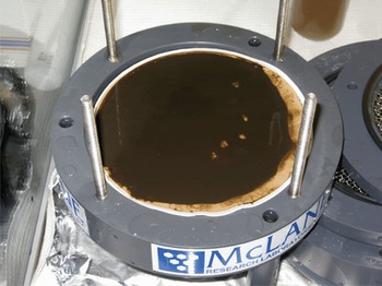
Fig. 5. Fine-grained sediments collected on the finest filter, 0.2 μm, of the McLane in situ filtration unit.

Sediment coring

The first corer we deployed in the SLW borehole was the UWITEC gravity multi-corer. It consists of three 60 µm diameter, 50 cm-long sampling tubes with automatic core catchers and is designed to enable sampling of soft sediments with preservation of the sediment/water interface. The entire assembly is relatively large, not streamlined, and quite light. Consequently, we experienced seven unsuccessful attempts at deploying the multi-corer because it either got stuck in the borehole or could not advance beyond the ice layer that formed at the air/water interface. Given these problems, the decision was made to put the drill back into the SLW borehole for an up-and-down ream cycle which lasted for ~24 hours (Fig. 2).

Sediment coring was the key objective for the second phase of scientific borehole operations at SLW (Fig. 2). The NIU multi-corer was deployed immediately after borehole reaming, and on three deployments it returned two sediment cores in each run (Fig. 6). The cores were up to 0.4 m in length. One of the multi-corer samples was used to collect pore waters for chemical analyses using Rhizon samplers (Reference Seeberg-Elverfeldt, Schlüter, Feseker and KöllingSeeberg-Elverfeldt and others, 2005). Later, in the second phase of scientific operations, we deployed the borehole piston corer with a 3 m-long barrel. It collected a 0.8 m-long core with a diameter of 58 mm.

The third sediment corer used was the 10 cm diameter, 5 m-long percussion corer. Due to malfunction of its smart winch, this was used essentially as a gravity corer, and collected 0.4 m-long samples. Between the first multi-corer deployment and the sampling with the percussion corer, the SLW borehole moved by ~1 m horizontally (Fig. 2).

Geothermal probe

It is difficult to constrain geothermal fluxes from basal temperature profiles measured in boreholes drilled in ice, and such estimates are associated with large uncertainties (e.g. supplementary material for WAIS Divide Project Members, 2013). Antarctic geothermal flux distribution is crucial to understanding the tectonic evolution of Antarctica, the dynamics of its ice sheet, and its subglacial hydrology, but it is only constrained by geophysical models, which yield quite disparate results (cf. Reference Shapiro and RitzwollerShapiro and Ritzwoller, 2004; Reference Maule, Purucker, Olsen and MosegaardMaule and others, 2005). The geothermal probe was designed to penetrate sediments at the bottom of SLW and measure precisely the vertical temperature gradient (Reference FisherFisher and others, 2003; Reference Heesemann, Villinger, Fisher, Tréhu and WhiteHeesemann and others, 2006). In combination with direct laboratory measurements of thermal conductivity on sediment samples, the observed sub-glacial vertical temperature gradient will be used to calculate geothermal flux.

Borehole sensor string

Installation of the borehole sensor string early on 1 February 2013 represented the final stage of scientific operations in the SLW borehole. The string contains one three-axes borehole seismometer (Geosig), three vertical-axes geophones (one at the very bottom of the string, one 100 m above and one 600 m from the bottom) plus an 800 m-long fiber-optic distributed temperature sensor (DTS). Due to environmental stewardship, the bottom of the string was installed ~20m above the ice base, rather than all the way to the bed. The lowest point of the string corresponds to the bottom of the DTS and contains the Geosig borehole seismometer as well as one of the geophones. The sensor string was left to freeze-in, and the top of the borehole was covered for safety. Power and data connections for the borehole sensors are located on the surface. Both seismic sensors and the DTS survived the borehole freezing process, and data were collected from them during the 2013/14 season.

Operational issues

Whereas the WISSARD Science Team planned for the potential risk of borehole diameter shrinkage due to refreezing, formation of ice at the top of the borehole was not managed. Consequently, scientific operations in the SLW borehole were impacted by freezing at the air/water interface.

To mitigate the risk from lateral borehole refreezing, we requested a borehole diameter which exceeded by >0.2 m the diameter of our largest scientific equipment. Moreover, the planned scientific borehole timeline prioritized, whenever there were no overriding scientific considerations, the large-diameter tools. Based on Reference KociKoci (1984, fig. 4), we estimated that borehole freezing rates would decrease from ~8 cm d^–1 on day one to about 4 cm d^–1 on day four for the mean annual temperature of –25°C at the SLW site. Freezing rates should decrease to nil at the base, where ice temperature is near its pressure-melting point (Reference EngelhardtEngelhardt, 2004).

Freezing at the top of the SLW borehole water column resulted in significant disturbance to the planned operational sequence, but we found no quantitative treatment of this problem in published literature. A simple equation quantifying the growth in ice thickness, h, is given by Reference StefanStefan (1891):

(1)

where Ki is the thermal conductivity of ice (2.1 Wm^–1°C–¹), T is the difference between the freezing point of water and air temperature right above the ice layer, t is time, L is the latent heat of freezing (333.5 kJ kg^–1) and ρ is density (917 kgm^–3). Equation (1) shows that in just one day, the ice layer reaches ~0.03 m thickness, with air temperature being just 1°C below freezing. Data from the geothermal probe, which was deployed about a day after borehole reaming, show that air temperature in the borehole was below -4°C.

Lake ice studies indicate that the load capacity of an ice layer scales with the square of its thickness (Reference BealtosBealtos, 2002):

(2)

where F is the ‘safe’ short-term load (kN) and Ci is an empirical constant with units of stress, given by Reference BealtosBealtos (2002, p. 206) as 1790 kPa. Equation (2) has been developed and calibrated for horizontally extensive ice layers, whereas we consider an ice layer in a borehole with radius R. However, it should still be applicable as long as h « R. Even if we take h = 0.03 m, as calculated above, such a layer can support a piece of equipment with mass of ~200 kg.

Growth of an ice layer at the top of a water-filled borehole can be hindered by supplying hot water at the water/air interface. It is sufficient to keep an ice layer thin enough so that it can be penetrated by even light instrumentation. For instance, a 0.002 m-thick ice layer will be broken by a mass greater than 2 kg. The rate of hot-water input, q (kgs–¹), needed to balance conductive heat loss through an ice layer of thickness h can be estimated from

(3)

where the first ratio on the right-hand side represents a linear temperature gradient across the ice layer, the second term is the ratio of ice thermal conductivity to heat capacity of water (cp = 4218J kg–¹ K–¹) and the third term is the ratio of borehole area to the temperature of drill water, Tdw. Even for T=-200C, it would take just 1 L min^–1 of drill water with a temperature of 85º C to keep an ice layer from growing beyond 0.002 m thickness in a borehole of 0.6 m diameter. However, this would mean deploying an additional hose into the borehole, which could risk entanglement with instruments being deployed down-hole.

Water properties and lake depth

Our first opportunity to examine the transition from borehole water to subglacial water came during the deployment of the MSLED camera (Fig. 2). It went through the air/water interface 78 m below the ice surface. Borehole water first appeared turbid at ~520 m depth, and turbidity increased markedly near the bottom of the borehole. High turbidity made it difficult to determine the depth to the ice base, which was picked to be at -800 m below surface based on decrease in image brightness, presumed to be due to camera lights no longer reflecting from borehole walls. After an estimated 1.6 m of additional cable pay-out, the camera rested on the lake bottom, imaging the top of relatively soft sediments (Fig. 3). It is difficult to quantify the uncertainty on this visual water depth estimate. Below we use CTD data as an additional constraint.

Figure 4 shows the vertical profile of salinity (psu), including a detailed view of the lowermost 10m of the borehole. For reference, standard sea-water salinity is 35 on the psu scale, whereas the maximum salinity in Figure 4 is almost 100 times lower. Hence, all water encountered by the CTD, including the subglacial cavity water, is quite fresh, with subglacial water being similar in salinity to a lower Colorado River reservoir. Pure meltwater generated during drilling has nil salinity, with psu values staying at the limit of detectability (<0.002 psu) above 530 m water depth. This observation is consistent with the very low ion concentration found in the Siple Dome ice core (Reference MacGregor, Winebrenner, Conway, Matsuoka, Mayewski and ClowMacGregor and others, 2007).

The average salinity of borehole water below 530 m is 0.28 psu, about three orders of magnitude higher than the salinity of drill meltwater. Assuming that this average salinity resulted from mixing of drill meltwater (0.002 psu) with subglacial water (0.37-0.41 psu) (Fig. 4), then the latter constitutes 25-27% of borehole water below 530 m. If the average borehole diameter was the design diameter of 0.6 m, then we estimate that about 20 m³ of subglacial water entered the borehole before our first CTD cast. This value exceeds our prior estimate of 8 m³ entering the borehole during the drill breakthrough. The initial influx may have been at the 20 m³ level because of the presence of the return pump borehole next to the main hole, or subglacial water continued to enter the borehole during reaming.

The total water column depth measured by the CTD when it was resting at the bottom of SLW was 724.6 ± 0.7 m. This means that the lake bottom was 802.6 ± 0.8 m below ice surface. As the CTD was being lowered into the borehole, water salinity had very low scatter down to 798.4± 0.8 m below the surface. A distinct kink in the salinity curve is seen at -800 m. Analysis of the corresponding CTD water temperature data, not shown here, indicates an approximately isothermal water layer in the lowermost 2.2 m of the record. Based on these salinity and temperature data, we interpret that the subglacial water layer was 2.2 m thick beneath the SLW borehole. This is slightly higher than the 1.6 m water thickness estimated with the borehole camera.

The minimum water temperature of -0.55°C was recorded in the borehole by the CTD unit at a pressure of 7019±7kPa (Sea-Bird Electronics, 2013) and salinity of 0.31 psu. With salinity at <1% of sea-water salinity, at most 0.02°C of freezing-point depression can be due to solutes. Most of the observed depression, about -0.53°C, is attributable to the pressure dependence of the freezing point, with a proportionality coefficient of 75.5 x10^–8°CPa^–1. This coefficient is within 2% of the value of 74.2 x 10^–88CPa–¹ given by Reference Cuffey and PatersonCuffey and Patterson (2010) for pure water. This slight discrepancy may result from the presence of dissolved gas in subglacial water (Fig. 6; Reference Tulaczyk, Kamb and EngelhardtTulaczyk and others, 2001).

Fig. 6. Multi-corer sediment core in a transparent liner with a ruler in centimeters on the right-hand side. The dark spots are interpreted as gas bubbles formed as a result of core depressurization as it is brought up to the surface (Reference Tulaczyk, Kamb and EngelhardtTulaczyk and others, 2001).

Subglacial cavity and its sedimentary environment

Radar and seismic geophysical surveys provided evidence for the presence of a subglacial water layer with horizontal extent corresponding closely to the footprint of SLW inferred previously from ice surface elevation changes (Reference Fricker, Scambos, Bindschadler and PadmanFricker and others, 2007; Reference Fricker and ScambosFricker and Scambos, 2009; Reference Christianson, Jacobel, Horgan, Anandakrishnan and AlleyChristianson and others, 2012; Reference HorganHorgan and others, 2012). Borehole observations yield direct confirmation that this water layer interpreted from remote-sensing and surface geophysical data does exist in the study area. However, they do not confirm the inference drawn from active-source seismic profiling that the subglacial water column is 8 ± 2 m thick at the drill site (Reference HorganHorgan and others, 2012, fig. 7). This discrepancy is difficult to explain by changes in lake thickness in the 2 years between seismic surveys and drilling (Fig. 1b).

This opportunity to double-check Antarctic subglacial conditions inferred from surface active-source seismic investigations represents a cautionary note that emphasizes the resolution limitations and potential non-uniqueness of geophysical methods. Conceivably, SLW depth distribution is sufficiently variable on horizontal scales smaller than the resolution of the seismic survey, ~180m (Reference HorganHorgan and others, 2012, p. 203), for the borehole to encounter a local high in the lake bed that is not resolvable in the seismic data. Alternatively, limits on vertical resolution may have made it impossible to distinguish between the thin water layer and relatively soft subglacial sediments with similar seismic velocities.

We conjecture that the bowl-shaped sub-ice reflector imaged by Reference HorganHorgan and others (2012) may not represent the bottom of a water body but a boundary between the relatively porous and weak sediments cored by us and some denser and/or more rigid geologic substratum. Given its geometry and spatial coincidence with the surface expression of SLW, it is plausible that this reflector delineates an erosional boundary which used to be the bottom of the lake. Over time this shallow basin may have become largely filled with sediments.

The sediment cores recovered from SLW are composed of a macroscopically structureless diamicton and are similar to the subglacial tills recovered previously from beneath Siple Coast ice streams (Reference Scherer, Aldahan, Tulaczyk, Possnert, Engelhardt and KambScherer and others, 1998; Reference Tulaczyk, Kamb, Scherer and EngelhardtTulaczyk and others, 1998, Reference Tulaczyk, Kamb and Engelhardt2000). Sediment shear strength, measured in June 2013 on a split percussion core with a handheld penetrometer, was also similar to previously measured values (Reference Tulaczyk, Kamb and EngelhardtTulaczyk and others, 2001), with 2 kPa near the core top and rising to ~6 kPa at 0.2 m below surface. At this point we have no observational basis to decide if these sediments are true glacial tills, i.e. have been brought to the location where they were sampled by ice, or represent till material that has been redeposited by subaqueous flows in the lake basin. Such redeposition has been proposed to be one of the leading mechanisms for sub-ice sedimentation in SLW (Reference Bentley, Christoffersen, Hodgson, Smith, TulaczykSand Le Brocq, Siegert, Kennicutt and BindschadlerBentley and others, 2013).

No clear evidence of sedimentation from settling is present in the collected SLW cores, although we observed abundant suspended particles in subglacial water. One interpretation is that this water turbidity resulted from hot-water drilling through debris-laden basal ice. Reference Christoffersen, Tulaczyk and BeharChristoffersen and others (2010) estimated that basal ice of the neighboring Kamb Ice Stream contains debris equivalent to a ~2 m-thick sediment layer. However, the lack of positive evidence for coarse sediment settling at the bottom of the lake (Fig. 3) favors the alternative explanation that lake water was turbid even before drilling. Similarly, the lack of a coarse lag on the sampled lake floor indicates that influx of subglacial water into the borehole at the time of its completion either did not mobilize bottom sediments or did it only over an area small enough for the coring to miss the disturbed zone (Fig. 2).

High turbidity is common in glacially fed streams and lakes (e.g. Reference Milner and PettsMilner and Petts, 1994), so it would not be surprising if SLW water is turbid in its natural state. Detailed particle-size analyses of till samples from upstream of SLW demonstrated that 20–25% of these sediment samples were smaller than 0.5 µm (Reference Tulaczyk, Kamb, Scherer and EngelhardtTulaczyk and others, 1998). Such fine particles may stay in suspension practically indefinitely, due to Brownian collisions with water molecules (Reference RamaswamyRamaswamy, 2001). Subglacial water entering SLW may bring very fine particles that do not settle out and leave no sedimentary signature at the lake bottom.