


Notation
a(x, t) Accumulation rate
b(x) Bed topography
g Gravitational acceleration
h(x,t) Ice thickness
k Boundary elevation rate
n Power in Glen's flow law
q(x, t) Ice flux
s(x, t) Ice-surface elevation
t Time
u(x,z) Horizontal ice velocity
x Distance along flow
z Distance above bed
A Depth-averaged flow parameter
E Matrix of eigenfunctions
G Green's function matrix for accumulation perturbations
H(x) Eigenfunction/spatial component of h1
M Discrctizcd version of θ
Q(x) Spatial component of q1
R Divide migration rate
T(t) Temporal component of h 1, a 1, q 1
X,d Divide position
a(x) Spatial component of a 1
β Scaled accumulation gradient
ϒ ![]()
λ Eigenvalue
ρ Ice density
σ(x,y) Shear stress
τ Time constant
φ Rate of change in scaled accumulation gradient β
θ Linear perturbation operator
Λ Diagonal matrix of eigenvalues
Superscript/Subscript
* Initial condition
~ Reference value
0 Zeroth order (steady-state)
1 Perturbation d Divide position
ν Volumetric
Η Hindmarsh
L Left
R Right
W Weertman
Introduction
The motion of ice divides can be caused by changing conditions at ice-sheet boundaries. A record of ice-divide position may be a delayed and smoothed representation of boundary forcing. If the relationship between divide motion and boundary forcing can be established, then one could infer boundary forcing from a record of divide position, or predict divide position for a given boundary forcing. Ice divides are also theoretically associated with a narrow zone of anomalous ice flow which causes isochrones to be warped convex-up beneath steady divides (Raymond, 1983; H vidberg, 1996). Small variations in divide position compared with the icc-shcct span may cause perturbations to the flow field and complicate the interpretation of ice cores obtained at ice divides. The sensitivity of divide position to boundary forcing is therefore relevant to possible identification of forcing mechanisms occurring at ice-sheet boundaries and to interpretation of ice cores obtained at ice divides.
Weertman (1973) investigated the effect of simple changes in ice-sheet span and accumulation rate on divide position, with the finding that steady-state divide position is most sensitive to changes in ice-sheet span and less sensitive to the spatial pattern of accumulation. Hindmarsh (1996b) characterized the sensitivity of divide position to stochastic asymmetric accumulation forcing and found that the relaxation time-scale of divide position to such forcing is about 1/16 of the fundamental thickness/accumulation-rate (h/a) time-scale. Reference Anandakrishnan, Alley and WaddingtonAnandakrishnan and others (1994) used inverse techniques to estimate that the Greenland ice divide may have shifted by about 40 km and thinned by 50 m over the last Glacial cycle from changes in margin position and accumulation rate. Cufley and Clow (1997) estimated the effect of margin expansion and retreat on the divide elevation in central Greenland over a Glaciol cycle, with a diffusive relaxation time of about 1900 years, about 1/5 of the fundamental h/a time-scale.
In this paper, we determine the sensitivity of divide position of Siple Dome, the ice ridge between Ice Streams C and D, West Antarctica, to more subtle forcing at its boundaries (Fig. 1). A deep ice core is being obtained near the present summit for palcoclimatc analysis. Recent migration of the Siple Dome divide northward toward Ice Stream D at a rate of 0.05-0.50 m a−1 over the past several thousand years has been inferred from analysis of the pattern of internal layers near the divide which have been detected with an ice-penetrating radar (Nereson and Raymond, in press; Nercson and others, in press). We identify probable causes of this subtle divide motion by quantifying the effects of small changes in accumulation pattern and small changes in the elevation of the lateral boundaries of Siple Dome (an indicator of ice-stream activity around Siple Dome) on the divide position.
Linearized Ice-Sheet Equation
Wc consider a linearized perturbation about a two-dimensional Vialov-Nye ice-sheet solution. Standard ice-flow models do not generally conta in the scale of resolution required to simulate small changes in divide position (<0(h)). A linearized perturbation allows simulation of small-scale divide motion as it permits explicit tracking of divide position.
Mathematical development of the linearized ice-sheet evolution equation is given in Nye (1959) and Reference HutterHutter(1983). The main points are summarized here.The time-dependent evolution equation for a two-dimensional ice sheet is
where h(x, t) is the ice-sheet thickness, q(x, t) is the ice flux, a(x,t) is the mass balance, and x is the distance along flow. For an ice sheet deforming in laminar flow with shear stress
Fig. 1. Map of West Antarctic Siple Coast ice streams, showing Siple Dome and Ice Streams C and D.
and flow relation
we obtain an expression for the ice flux q,

where s(x, t) is the surface profile, obtained by the sum of the ice thickness h(x, t) and bed elevation b(x), z is the distance above the bed, ice density ρ = 917 kg m −3, gravitational acceleration g = 9.8 m s−2, depth-averaged flow law parameter A is prescribed, n = 3, and m = n + 2. Substituting

yields the Vialov-Nye (VN) ice-sheet evolution equation,
The standard steady-state Vialov profile is obtained when ![]() and a = a0
is a constant (Vialov, 1958).
and a = a0
is a constant (Vialov, 1958).
We are interested in the effect of small perturbations in thickness h and accumulation a on the ice-sheet geometry. We expand h and a such that

where ![]() . Substitution into Equation (4) yields a corresponding flux expansion,
. Substitution into Equation (4) yields a corresponding flux expansion,
The zeroth-order state is defined to be steady state such that

Substituting Equations (7), (8) and (9) into Equation (6) and keeping only first-order terms yields the linearized perturbation equation which we solve to determine the ice-sheet response to small perturbations:

where ![]() . When m = 0 and n = 1, the standard linear diffusion equation is obtained (e.g. Boycc and DiPrima, 1986), and we expect diffusive-type behavior when m = 5 and n = 3 (Nye, 1959). It is convenient for developments in later sections to write Equations (10) and (11) in operator form as
. When m = 0 and n = 1, the standard linear diffusion equation is obtained (e.g. Boycc and DiPrima, 1986), and we expect diffusive-type behavior when m = 5 and n = 3 (Nye, 1959). It is convenient for developments in later sections to write Equations (10) and (11) in operator form as
where

Calculation of Normal Modes
Since Equation (10) (or (12)) is a linear differential equation, its general solution can be expressed as a superposition of solutions to the homogeneous equation
where h 1 0 at the lateral boundaries of the domain (Reference Boyce and DiPrimaBoyce and DiPrima, 1986). Following Hindmarsh (1996a, b, 1997a, b), we assume a separable solution,
Because the problem is linear, we may also write:
Substituting Equations (15) and (17) into the homogeneous equation (14) allows us to separate the time-dependent and the space-dependent equations by use of a separation constant, or eigenvalue λ:

where

The solution for the time-dependent component of Equation (18) is Τ = Τ* exp(λt), where Τ* is an initial condition. The eigenvalue λ represents an inverse relaxation time-constant for the spatial solution H(x), provided λ < 0.
The solution H(x) is a spatial response function, or ci-genfunction, associated with the time-constant given by λ. These spatial solutions are the normal modes of the ice sheet and are found by solving the spatial component (righlhand side) of Equation (18),

Following Hindmarsh (1996a, 1997b), we discretize Equation (20) according to the method of finite differences and solve the resulting algebraic eigenvalue problem written in matrix form as:
where A is a diagonal matrix of eigenvalues λi, M is the discretized version of the operator θ and Η is a vector of perturbations sampled at Ν discrete points in x. Specifically, M is a tridiagonal matrix whose values are found by evaluating the discretized version of the operator θ at N-2 points in x. The solution is found by finding the eigenfunctions and ei-genvalues of M. We construct a matrix E whose ith column is the eigenfunction Hi(x) corresponding to λ i and a vector Τ — Τ* exp(At), where T* is an initial condition. The general solution to the perturbation equation (12) can be written in matrix form as a linear combination of the temporal and spatial solutions to the homogeneous equation (14):

Estimating Divide Motion
We are particularly interested in flow the position of the ice divide is affected by perturbations. Following Hindmarsh (1996b), the evolution of divide position where ![]() can be written as
can be written as
where R is the divide migration rate. in an increment of time, δt the divide motion is then

This relation implies that divides with high curvature are less sensitive to a given perturbation s1
Equation (24) is technically invalid because it ignores the fact that the divide curvature ![]() is singular for (VN) ice-shect profiles. in general, accurate calculation of flow near the divide requires special mathematical treatment because the standard (VN) ice-flow model is invalid there. While the separate solutions to symmetric and antisymmetric perturbations have been calculated while fully accounting for the divide singularity for the VN ice-sheet solution (e.g. Hindmarsh, 1997a), the general problem has not been solved. We ignore the effect of the divide singularity and estimate divide curvature from a Taylor expansion of a discretized ice sheet. This approximation results in a small error in the estimation of divide position.
is singular for (VN) ice-shect profiles. in general, accurate calculation of flow near the divide requires special mathematical treatment because the standard (VN) ice-flow model is invalid there. While the separate solutions to symmetric and antisymmetric perturbations have been calculated while fully accounting for the divide singularity for the VN ice-sheet solution (e.g. Hindmarsh, 1997a), the general problem has not been solved. We ignore the effect of the divide singularity and estimate divide curvature from a Taylor expansion of a discretized ice sheet. This approximation results in a small error in the estimation of divide position.
We quantify this error by comparing our solution to an analytic solution fora special case. Weertman (1974) considered the effect of a step change in accumulation rate on both right and left sides of an initially symmetric VN ice-sheet profile, and determined that the total divide motion is

where ![]() and
and ![]() and
and ![]() , are spatially const ant accumulation rates for the right and left sides of the ice sheet, respectively. Hindmarsh (1997a) showed that the linearized solution for divide movement caused by imposing a step increase in
, are spatially const ant accumulation rates for the right and left sides of the ice sheet, respectively. Hindmarsh (1997a) showed that the linearized solution for divide movement caused by imposing a step increase in ![]() is
is

A comparison between the analytic solutions ![]() and the solution Xd
given by Equation (24) for a given
and the solution Xd
given by Equation (24) for a given ![]() and for a range of discretization intervals dx shows that all results agree to within 10%. This error is smaller than errors due to uncertain accumulation rate and flow properties (leading to errors in
and for a range of discretization intervals dx shows that all results agree to within 10%. This error is smaller than errors due to uncertain accumulation rate and flow properties (leading to errors in ![]() ), and is acceptable since the flow divide and topographic divide do not exactly correspond for real ice sheets (Raymond, 1983). The exact solution of the problem that respects the divide singularity would probably not increase the accuracy of the physical solution.
), and is acceptable since the flow divide and topographic divide do not exactly correspond for real ice sheets (Raymond, 1983). The exact solution of the problem that respects the divide singularity would probably not increase the accuracy of the physical solution.
Normal Modes of Siple Dome
Field measurements made in 1994 and 1996 show that Siple Dome is essentially a two-dimensional ridge about 1000 m thick and 100 km wide overlying relatively flat bedrock (Raymond and others, 1995). Wc are therefore justified, to first order, in applying this two-dimensional linearized perturbation model to Siple Dome. Figure 2 shows the zeroth-order geometry (h
0 and b) for two similar icc-shect profiles for which we calculate normal modes: a theoretical flat-bed VN ice sheet, and the actual Siple Dome (SDM) ice sheet from field measurements of surface and bed topography (Raymond and others, 1995). These two geometries are used to illustrate the sensitivity of our results to variations in ice-sheet shape. We choose ![]() and
and ![]() to calculate the VN ice-sheet geometry from Equation (6). The domain is truncated at ± 47 km from the summit with x =0 at the divide, approximately corresponding to the full span of Siple Dome.
to calculate the VN ice-sheet geometry from Equation (6). The domain is truncated at ± 47 km from the summit with x =0 at the divide, approximately corresponding to the full span of Siple Dome.
We obta in the zeroth-order flux q
0 directly by integrating the accumulation rate.This approach does not require explicit knowledge of the flow parameter A, although A can be deduced from the zeroth-order accumulation rate and geometry. Measurements from snow pits and shallow cores show that the accumulation rate at the summit of Siple Dome is about 0.11-0.13 m a−1 ice equivalent (Reference Mayewski, Twickler and WhitlowMayewski and others, 1995) with a south-north accumulation gradient giving higher accumulation to the north (personal communication from K. Kreutz, 1997). For convenience, a reference accumulation rale àis defined lobe that at the divide: ![]() .
.
Fig. 2.
Ice-sheet geometries used to calculate h₀ and s₀ in Equation (11). The dashed profile corresponds to a symmetric Vialov-Nye profile with ![]() ice equivalent, and a half-width of 47 km. The solid profile corresponds to the Siple Dome profile determined from radar and GPS measurements (Raymond and others, 1995).
ice equivalent, and a half-width of 47 km. The solid profile corresponds to the Siple Dome profile determined from radar and GPS measurements (Raymond and others, 1995).
Figure 3 shows the slowest two ice-sheet modes found by solving Equation (21), assuming constant accumulation rate for each ice-shect profile shown in Figure 2. The eigenfunc-tion associated with the largest non-zero eigenvalue (labeled Mode I; Fig. 3) is the first dynamic ice-sheet mode and represents the slowest volumetric response of the ice sheet. Its time-scale (![]() ) is associated with the time it takes for the ice sheet to relax to a steady state after a perturbation. The second mode is the slowest mode representing divide position by virtue of its non-zero slope at the divide. Additional modes representing the ice-sheet response at higher wavenumbers have faster response times (< 102 years) and are not shown in Figure 3. There are two “solutions” to Equation (14) which correspond to the case where Q = constant and which have A = 0 (see Equation (20)). These “solutions” violate the boundary condition that h1 = 0 at the lateral boundaries of the domain, and are therefore discarded as solutions which define the ice-sheet modes. However, these functions will be valid solutions when we consider perturbations with non-zero values at the boundaries.
) is associated with the time it takes for the ice sheet to relax to a steady state after a perturbation. The second mode is the slowest mode representing divide position by virtue of its non-zero slope at the divide. Additional modes representing the ice-sheet response at higher wavenumbers have faster response times (< 102 years) and are not shown in Figure 3. There are two “solutions” to Equation (14) which correspond to the case where Q = constant and which have A = 0 (see Equation (20)). These “solutions” violate the boundary condition that h1 = 0 at the lateral boundaries of the domain, and are therefore discarded as solutions which define the ice-sheet modes. However, these functions will be valid solutions when we consider perturbations with non-zero values at the boundaries.
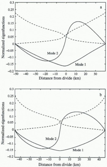
Fig. 3. Slowest ice-sheet normal modesfrom solution to Equation (14) for (a) the SDM ice-sheet geometry and (b) the V.N ice-sheet geometry shown in Figure 2. Accumulation rate, do = 0.10 m a−1 ice equivalent, is assumed constant in both cases. The volumetric response mode and divide position response modes are labeled Mode 1 and Mode 2, respectively. Solutions with zero eigenvalue (no intrinsic dynamics), which permit external forcing of boundary elevation, are denoted by dashed curves. The similarity between the two ice sheets shows that the response modes are relatively insensitive to small variations in surface and bed topography.
The relaxation time-scales associated with the slowest modes are shown in Table 1. The volumetric response time-scale ![]() is 450-800 years, and the divide position response
is 450-800 years, and the divide position response
Table 1.
Response-time constants in rears for slowest modes (volumetric response ![]() and divide position response
and divide position response ![]() for VN and SDM ice-sheet profiles with various grid spacings and accumulation patterns
for VN and SDM ice-sheet profiles with various grid spacings and accumulation patterns ![]() in ma−1 ice equivalent
in ma−1 ice equivalent

time-st ale ![]() is twice as fast at 200-350 years. Both are much less than the fundamental h₀/a₀ time-scale (~104 years). Increasing the accumulation rate shortens the fundamental time-scale and leads to a corresponding decrease in the mode relaxation time-scale. Because our domain is truncated with non-zero thickness at its boundaries, the volumetric relaxation time-scales are almost twice as fast as those found in Hindmarsh (1997a). in our case, the divide-to-margin ice thickness is about half that for a full non-truncated ice sheet so that the time-scales are correspondingly scaled by about a factor of 2. The values in Table 1 are comparable to those calculated using equations from CulTey and Clow (1997). Using values appropriate for Siple Dome, they estimate
is twice as fast at 200-350 years. Both are much less than the fundamental h₀/a₀ time-scale (~104 years). Increasing the accumulation rate shortens the fundamental time-scale and leads to a corresponding decrease in the mode relaxation time-scale. Because our domain is truncated with non-zero thickness at its boundaries, the volumetric relaxation time-scales are almost twice as fast as those found in Hindmarsh (1997a). in our case, the divide-to-margin ice thickness is about half that for a full non-truncated ice sheet so that the time-scales are correspondingly scaled by about a factor of 2. The values in Table 1 are comparable to those calculated using equations from CulTey and Clow (1997). Using values appropriate for Siple Dome, they estimate ![]() at about 750 years. The fact that the VN ice sheet and the Siple Dome ice sheet have similar eigenvalues and cigenfunctions shows that the ice-sheet response is relatively insensitive to small variations in the zeroth-order ice-sheet shape or the presence of moderate bed topography.
at about 750 years. The fact that the VN ice sheet and the Siple Dome ice sheet have similar eigenvalues and cigenfunctions shows that the ice-sheet response is relatively insensitive to small variations in the zeroth-order ice-sheet shape or the presence of moderate bed topography.
These short time-scales indicate that Siple Dome responds quickly to boundary forcing. Information about changes in ice-stream activity or in the spatial pattern of accumulation prior to a few thousand years ago is no longer contained in the geometry of Siple Dome. The time-scale associated with divide position is much shorter, indicating that the Siple Dome divide motion is neither a response to a distant past event, such as the transition from the Last Glaciol Maximum to the Holocene, nora response toan abrupt event in the past few thousand years. The divide motion is more likely associated with an ongoing, sustained forcing.
Response to Boundary Elevation Perturbation
There is evidence that the ice streams bounding Siple Dome have recently changed their activity. The lower part of Ice Stream C essentially stopped stream flow about 130 years ago and is currently thickening at the accumulation rate (Reference Retzlaff and BentleyRetzlaff and Bentley, 1993). A linear feature on the north flank of Siple Dome near Ice Stream D is likely a former ice-stream margin that ceased flow about 103 years ago (Reference Jacobel, Scambos, Raymond and GadesJacobel and others, 1996). We expect that once stream flow ceases/begins, the ice streams may thicken/thin and change the elevation at the boundaries of Siple Dome. We consider two cases: (I) an increase in elevation at the ice-sheet margin sufficiently fast that it can be represented as an instantaneous change, and (2) a steady increase in margin elevation at a constant rate.
The effect of perturbing the elevation of the ice-sheet boundary is found by solving Equation (12) as an initial value problem. For the first case, we specify as the initial condition a spike in elevation at the boundary ![]() for all x except at the boundary). We hold the boundaries fixed at these initial values for t>0. Since h1= ET by Equation (22) the initial condition is
for all x except at the boundary). We hold the boundaries fixed at these initial values for t>0. Since h1= ET by Equation (22) the initial condition is
and the solution is
Figure 4 shows the ice-sheet response for an instantaneous arbitrary increase in elevation of the Ice Stream D-sidc boundary by about 10% of the total ice thickness (100 m).The shape of the steady-state ice-sheet response corresponds to one of the cigenfunctions with zero eigenvalue (Fig. 3). This is expected since these eigenfunctions are the Fig. 4. Evolution of thickness perturbation h1 (x, t) for an instantaneous 100 m increase in elevation of the margin of Siple Dome near Ice Stream D, plotted every 200 years.

Fig. 4.

Fig. 5.
(a) Evolution of divide elevation for an instantaneous 100 m increase in elevation of the ice-sheet boundary nearest Ice Stream D. The characteristic (1-1/e) relaxation time for all cases is about 500-800years, (b) Evolution of divide posi-tion with a relaxation time of about 200-350 years. (A) SDM geometry, ![]() ; (B) SDM geometry, a0(x) = 0.15m a−1 ; (C) SDM geometry,
; (B) SDM geometry, a0(x) = 0.15m a−1 ; (C) SDM geometry, ![]() SDM geometry,
SDM geometry, ![]() ; (E) VN geometry,
; (E) VN geometry, ![]() . There is a response delay oj 100-200 years until the boundary perturbation affects the divide.
. There is a response delay oj 100-200 years until the boundary perturbation affects the divide.
only ones which will not exponentially decay over time (all other λ < 0).
figure 5a and b shows the divide elevation and divide position response for a range of initial conditions. There is a divide response delay of 100-200 years when the effect of boundary perturbation is propagating up the ice sheet and has not yet affected the divide (Reference Alley and WhillansAlley and Whillans, 1984). The characteristic time to reach steady state for each case is similar to the volumetric and divide position relaxation time-scales shown in Table l.The zeroth-order, reference accumulation rate ![]() affects only the response time-scales and thus the transient divide response. The final divide position and elevation are determined by the mode shapes which are independent of α and depend only on flow h₀ and a0 vary with x (e.g. compare curves A and B). Increasing the elevation of the Ice Stream D-side boundary by 10% of the scale thickness causes a 2~3% increase in divide ice thickness, and migration of the divide toward Ice Stream D by about 1 % of the total span. Since the problem is linear, a 20% elevation change would predict a 4-6% change in ice thickness and a 2% divide shift. Because the ice sheet is largely symmetric, a similar decrease in elevation of the Ice Stream C boundary would also produce the divide shift shown in figure 5b.
affects only the response time-scales and thus the transient divide response. The final divide position and elevation are determined by the mode shapes which are independent of α and depend only on flow h₀ and a0 vary with x (e.g. compare curves A and B). Increasing the elevation of the Ice Stream D-side boundary by 10% of the scale thickness causes a 2~3% increase in divide ice thickness, and migration of the divide toward Ice Stream D by about 1 % of the total span. Since the problem is linear, a 20% elevation change would predict a 4-6% change in ice thickness and a 2% divide shift. Because the ice sheet is largely symmetric, a similar decrease in elevation of the Ice Stream C boundary would also produce the divide shift shown in figure 5b.
This analysis of an instantaneous change in boundary elevation helps determine divide response characteristics, but may not be physically reasonable. in reality, the boundaries of Siple Dome probably change elevation over long time-scales. Moreover, we are particularly interested in what gradual boundary changes could produce the constant rate of divide migration inferred for Siple Dome. Since the divide response delay time is 100 200 years, it is likely that the Siple Dome divide is just now beginning to experience the effects of any thickening associated with the shut-down of Ice Stream G. Possible thickening associated with shut-down of the relict Ice Stream D margin would move the divide in the direction of the observed motion. Therefore, we wish to find the elevation rate k of the Ice Stream D-sidc boundary which produces the inferred Siple Dome divide migration rate. The solution is found by superposing solutions given by Equation (28) which we write in matrix form as
Figure 6 shows the migration rate deduced by solving Equation(29) for various elevation rates k and for various initial conditions. An elevation rate of 0.005-0.040 m a−1 (ice equivalent) produces the inferred migration rate and corresponds to elevating the right boundary 10-80 m in the past 2000 years. This result is not unique, however. Boundary changes producing a similar relative difference in elevation of the two sides would also match the inferred divide motion. For example, it is possible that the boundary adjacent to Ice Stream C has decreased in elevation sometime in the past few thousand years, as a result of a past change in Ice Stream C flow.

Fig. 6.
Steady-slate divide migration rates for various rates of boundary elevation. The rate of Siple Dome divide migration inferredfrom the pattern of internal layering (0.05-0.50 ma−1) is bounded by solid horizontal lines. (A) SDM geometry, ![]() ; (Β) SDM geometry,
; (Β) SDM geometry, ![]() ; (C) VN geometry,
; (C) VN geometry, ![]() . The divide migration rate depends only on flow a₀ and h₀ vary with x, and is independent of the reference accumulation rate
. The divide migration rate depends only on flow a₀ and h₀ vary with x, and is independent of the reference accumulation rate ![]() .
.
Response to Accumulation Rate Perturbation
Divide migration can also be caused by a change in the accumulation pattern. The ice-sheet response to such a perturbation is found by solving Equation (12) which we write in matrix form as
After using Equations (22) and (21) this becomes
and reduces to
Since Τ = T* exp At by Equation (18), we solve for T* given ai.
Again, we consider two cases: (1) the response of the ice sheet to an instantaneous accumulation rate perturbation, ![]() and (2) the response to a constant increase in the spatial accumulation gradient,
and (2) the response to a constant increase in the spatial accumulation gradient, ![]() where
where
is a prescribed constant. We fix the boundary elevations at their present values for both cases. The solution Τ for each case is found using standard analytical techniques for solving first-order ordinary differential equations. Upon using Equation (22) the ice-sheet response is:

for cases I and 2, respectively. The exponential terms in Equations (34) and (35) represent the transient ice-sheet response. At steady state (![]() ) these equations become
) these equations become
The quantity G = —ΕΛ−1Ε −1 is the Green's function for accumulation perturbations (Hindmarsh, 1997a).
Figure 7 shows the ice-sheel response to an instantaneous change in accumulation, ![]() where
where ![]() . Figure 8 shows the divide position response for various initial conditions for the same fractional accumulation perturbation β. There is no divide response delay time in this case, and divide evolution begins immediately with relaxation time-scales consistent with those in Table 1. Unlike margin perturbations, accumulation perturbations excite in general all ice-sheet modes which depend strongly on the characteristics of the zeroth-order ice-sheet configuration. The steady-state divide position is therefore more sen-sit ive to the initial ice-sheet geometry and the spatial pattern of accumulation, producing a 20% variation in Figure 8. However, like the case for margin elevation perturbations, the transient divide response is sensitive to
. Figure 8 shows the divide position response for various initial conditions for the same fractional accumulation perturbation β. There is no divide response delay time in this case, and divide evolution begins immediately with relaxation time-scales consistent with those in Table 1. Unlike margin perturbations, accumulation perturbations excite in general all ice-sheet modes which depend strongly on the characteristics of the zeroth-order ice-sheet configuration. The steady-state divide position is therefore more sen-sit ive to the initial ice-sheet geometry and the spatial pattern of accumulation, producing a 20% variation in Figure 8. However, like the case for margin elevation perturbations, the transient divide response is sensitive to ![]() for a given β, but the steady-stale response is independent of α.
for a given β, but the steady-stale response is independent of α.
We are interested in what gradual changes in accumulation pattern would cause the rate of divide motion inferred for Siple Dome. Specifically, we consider a gradual increase in the accumulation gradient over time producing lower accumulation rates toward Ice Stream C and higher rates toward Ice Stream D. Such a change could perhaps be linked to an evolution of the West Antarctic ice sheet which causes Siple Dome to emerge as a prominent topographic feature and so influence its climate, ora general change incirculation affecting Siple Dome climate over time. We use Equation (35), find the divide response for various values of φ and for various initial conditions, and show the predicted steady-state migration rate in Figure 9. Values for the rate of change in accumulation gradient (φα) ranging from 0.1 x 10 −9 to 1.5 x 10 −9 a 2 would produce the inferred divide migration rate (0.05-0.50 m a−1). At 10 km from the divide, these values correspond to a total increase/decrease in accumulation of 0.001 to 0.015 m a−1 (ice equivalent) in 1000 years. Accumulation changes in this range may be reasonable.

Fig. 7.
Evolution of SDM thickness perturbation h1 (x, t) for an instantaneous change in the accumulation pattern ![]() plotted every 200years.
plotted every 200years.

Fig. 8.
Evolution of divide position for an instantaneous accumulation perturbation ![]() SDM geometry,
SDM geometry, ![]() (Β) SDM geometry,
(Β) SDM geometry, ![]() ; (C) VN geometry,
; (C) VN geometry, ![]() . Solid and dashed curves correspond to
. Solid and dashed curves correspond to ![]() in a−1 and a = 0.15 m a−1 , respectively. Relaxation time-scales are about 200-350 years. For a given geometry and spatial accumulation pattern, the steady-state divide position is independent of a.
in a−1 and a = 0.15 m a−1 , respectively. Relaxation time-scales are about 200-350 years. For a given geometry and spatial accumulation pattern, the steady-state divide position is independent of a.

Fig. 9.
Steady-state divide migratimi rates for various rates of increase in accumulation gradient. The rate of Siple Dome divide migration (0.05-0.50 m a−1) is hounded by solid horizontal lines. (A) SDM geometry, ![]() ; (B) SDM geometry,
; (B) SDM geometry, ![]() a,
a, ![]() geometry,
geometry, ![]() . Solid and dashed curves correspond to
. Solid and dashed curves correspond to ![]() and
and ![]() , respectively. The range bounded by the inferred Siple Dome divide migration rate corresponds to a change in accumulation rate at 10 km from the divide of 0.001-0.015 m a−1 in 1000 years.
, respectively. The range bounded by the inferred Siple Dome divide migration rate corresponds to a change in accumulation rate at 10 km from the divide of 0.001-0.015 m a−1 in 1000 years.
Conclusions
Our results suggest that divide position at Siple Dome is quite sensitive to changes at its lateral boundaries and to changes in accumulation pattern. The divide motion inferred from the shapes of internal layers could be caused either by a change in elevation at its boundaries of less than 100 m or by a modest ongoing change in the accumulation gradient over the past several thousand years. Since the perturbations required to move the divide are small, and since the Siple Dome divide has moved only slightly in the past several thousand years, it is unlikely that Ice Stream C or D has changed its relative thickness dramatically in that time.
The divide position at Siple Dome would respond to abrupt forcing in a few hundred years (![]() ), with complete adjustment of the surface in a few thousand years (
), with complete adjustment of the surface in a few thousand years (![]() ). Therefore, only information about sustained forcing would persist in the geometry of Siple Dome for more than a few thousand years. The recent inferred migration of the Siple Dome divide is likely a response to ongoing changes in the bounding ice streams or the local climate rather than a response to an event in the distant past (>3 ka BP).
). Therefore, only information about sustained forcing would persist in the geometry of Siple Dome for more than a few thousand years. The recent inferred migration of the Siple Dome divide is likely a response to ongoing changes in the bounding ice streams or the local climate rather than a response to an event in the distant past (>3 ka BP).
Because of the delayed response to perturbations in margin elevation of 100-200 years, the Siple Dome divide has not yet been affected by elevation changes associated with the shut-down of Ice Stream C. However, a possible 20-80 m thickening associated with the shut-down of the relict Ice Stream D margin would be consistent with the inferred divide motion. Such an elevation change has not been measured. Photoclinometric analysis of satellite images indicates that the relict ice-strcam surface is about 50 m above the present level of Ice Stream D (Reference Scambos, Nereson and FahnestorkScambos and others, 1998), which is suggestive of recent thickening. This scenario is not unique. Small changes in the precipitation pattern over time are equally likely. Analysis of the pattern of internal layering at Siple Dome may help clarify which scenario has caused the inferred divide motion.
Acknowledgements
This work was funded by the U.S. National Science Foundation (grant No. OPP-9316807), the U.K. Natural Environment Research Council, and a European Science Foundation EISMINTexchange grant (No. 9614) which enabled essential collaboration between the authors. We gratefully acknowledge R. Jacobel, Τ Scambos, H. Conway and A. Gades for their contributions to SDM field data. We also thank D. Dahl-Jensen and R. Alley for their helpful comments.


