


Introduction
The lofty Himalaya with snow-clad peaks contain about 5000 glaciers of varying extents, covering an area of approximately 38 000 km2 (Reference KaulKaul, 1999). At global and continental scales, snow with its highly reflective nature and large surface cover has a great impact on regional climate, surface radiation balance and energy exchange and on the utilization of water resources. At regional and local scales and at the level of mountain-valley glaciers, snow cover has an impact on the local climate and the availability of water resources for industry, agriculture, domestic use, etc. (Reference König, Winther and IsakssonKönig and others, 2001; Reference Wang and LiWang and Li, 2003; Reference KargelKargel and others, 2005). In summer, the annual seasonal snow cover accumulating over the Himalayan glaciers and valleys forms an important source of replenishment for the major perennial river systems of northern India. The mapping and monitoring of snow and glacier characteristics is important for all these reasons (Reference KargelKargel and others, 2005).
Given the inaccessibility, vastness and harsh climatic conditions of snow/glacier areas, remote sensing appears to be the most appropriate tool for monitoring snow and glacier characteristics (Reference König, Winther and IsakssonKönig and others, 2001). Remote-sensing data can be acquired at a range of spectral, spatial and temporal resolutions. Depending on the spectral characteristics of the target to be mapped, remote-sensing data at different resolutions can be selected and various image-processing operations can be employed to extract the required information. The advent of improved satellite sensors (e.g. Terra ASTER (Advanced Spaceborne Thermal Emission and Reflection Radiometer), Terra MODIS (moderate-resolution imaging spectroradiometer) and Aqua MODIS) has accelerated remote-sensing based glaciological studies.
Remote sensing has varied applications in the field of glaciology, which is evident from a number of studies conducted to extract information from satellite data for specific glaciological tasks (Reference König, Winther and IsakssonKönig and others, 2001; Reference KargelKargel and others, 2005). Extensive studies have been carried out on mapping of snow and glacier cover employing different methods. These include
-
1. Mapping of glaciers and their retreat via manual digitization of glacier outlines (Reference Hall, Williams and BayrHall and others, 1992),
-
2. Image-ratioing based mapping of various snow and ice types (Reference Hall, Chang and SiddalingaiahHall and others, 1988; Reference Bronge and BrongeBronge and Bronge, 1999; Reference PaulPaul, 2001),
-
3. Normalized-difference snow index (NDSI) based snow- and glacier-cover estimation (Reference DozierDozier, 1989; Reference Hall, Riggs and SalomonsonHall and others, 1995; Reference Winther and HallWinther and Hall, 1999; Reference Silverio and JaquetSilverio and Jaquet, 2005),
-
4. Mapping dry and wet snow/ice cover (Reference Gupta, Haritashya and SinghGupta and others, 2005),
-
5. Snow and glacier mapping using image-classification techniques (Reference Aniya, Sato, Naruse, Skvarca and CasassaAniya and others, 1996; Reference Bronge and BrongeBronge and Bronge, 1999; Reference Sidjak and WheateSidjak and Wheate, 1999; Reference Slater, Slogett, Rees and SteelSlater and others, 1999),
-
6. Fractional snow-cover mapping (Reference Rosenthal and DozierRosenthal and Dozier, 1996; Reference Vikhamar and SolbergVikhamar and Solberg, 2003; Reference Salomonson and AppelSalomonson and Appel, 2004).
Remote-sensing data acquired from a number of sensors, such as the Landsat Thematic Mapper (TM) and Enhanced TM Plus (ETM+), SPOT (Système Probatoire pour l‘Observation de la Terre) Vegetation, the US National Oceanic and Atmospheric Administration (NOAA) Advanced Very High Resolution Radiometer (AVHRR), IRS (Indian Remote-sensing Satellite)-LISS (Linear Imaging Self-Scanning sensor) III and IV, Terra MODIS and Terra ASTER, were used in these studies. Most of the cited works deal with mapping of clean or only marginally contaminated snow/glacier surfaces.
However, many mountain glaciers in the Himalaya, Andes and Alaska ranges and on stratovolcanoes are covered with varying amounts of debris cover. A Himalayan glacier is typically composed of snow; ice; mixed ice and debris (MID); debris; and snowmelt water. Of these, debris cover is one of the most important constituents of a glacier system in controlling snowmelt runoff (Reference ØstremØstrem, 1959; Reference FujiiFujii, 1977; Reference Mattson, Gardner and YoungMattson and others, 1993), and the estimation of debris cover is crucial for understanding glacier mass balance (Reference MattsonMattson, 2000; Reference PeltoPelto, 2000). Debris cover near glacier snouts often portends the formation of moraine-dammed lakes, and debris cover over glaciers affects the response of glaciers to climatic changes (Reference Sakai, Takeuchi, Fujita and NakawoSakai and others, 2000). The changing extent of debris cover is thus considered an important indicator of glacier health (Reference Stokes, Popovin, Aleynikov, Gurney and ShahgedanovaStokes and others, 2007). In this context, mapping and regular monitoring of debris cover over glaciers from remote-sensing data is highly relevant.
Debris-Cover Studies using Remote-Sensing Data
Most of the glaciers in the Himalaya are covered with varying amounts of debris cover consisting of dust, silt, sand, gravel, cobble and boulders (Reference NakawoNakawo, 1979; Reference Fushimi, Yoshida, Watanabe and UpadhyayFushimi and others, 1980; Reference Mattson and GardnerMattson and Gardner, 1989; Reference Rana, Fukushima, Ageta and NakawoRana and others, 1996; Reference Adhikary, Nakawo, Seko and ShakyaAdhikary and others, 2000). Debris cover over glaciers is important for two main reasons:
-
1. Debris cover on glaciers hinders their mapping and has been recognized as a major problem in glaciological studies (Reference Whalley, Martin and GellatlyWhalley and others, 1986). The spectral response (i.e. reflectance) of debris cover in the form of digital number (DN) values stored within pixels of digital remote-sensing image data is related to the mixture of reflection from both debris and ice. Ice that is completely covered with debris may not be spectrally distinguishable from adjacent non-glaciated areas. Thus, actual glacier boundaries may be difficult to delineate in regions where they are thickly debris-covered, especially where debris-covered ice abuts talus slopes or old debris (Reference KääbKääb, 2005).
-
2. Debris cover has considerable influence on the glacier melting process, so its estimation is considered important for determining glacier runoff and evaluating water resources. Observations of ice ablation under a debris cover suggest that a very thin debris cover may accelerate melting, while an increasing thickness of debris, particularly in excess of a threshold thickness of approximately 0.02 m, inhibits melting (Reference ØstremØstrem, 1959; Reference LoomisLoomis, 1970; Reference FujiiFujii, 1977; Reference Mattson, Gardner and YoungMattson and others, 1993). Also, the temporal variation of debris cover over glaciers is correlated with changing regional climate and is hence considered an important indicator of glacier health and local climatic change (Reference Mihalcea, Mayer, Diolaiuti, Lambrecht, Smiraglia and TartariMihalcea and others, 2006; Reference Stokes, Popovin, Aleynikov, Gurney and ShahgedanovaStokes and others, 2007).
In view of the significance of debris cover in glaciology, various studies with different objectives such as mapping the extent of debris cover and its correlation with glacier recession (Reference Stokes, Popovin, Aleynikov, Gurney and ShahgedanovaStokes and others, 2007), mapping of different types of supraglacial debris cover (Reference Bishop, Shroder and WardBishop and others, 1995, Reference Bishop, Shroder and Hickman1999) and mapping of debris-covered glaciers (Reference Lougeay, Santeford and SmithLougeay, 1974; Reference Bishop, Kargel, Kieffer, MacKinnon, Raup and ShroderBishop and others, 2000, Reference Bishop, Bonk, Kamp and Shroder2001; Reference Taschner and RanziTaschner and Ranzi, 2002; Reference Paul, Huggel and KääbPaul and others, 2004; Reference Ranzi, Grossi, Iacovelli and TaschnerRanzi and others, 2004; Reference Buchroithner and BolchBuchroithner and Bolch, 2007; Reference Bolch, Buchroithner, Kunert, Kamp and GomarascaBolch and others, 2008) were carried out using remote-sensing data. For achieving these objectives, various techniques based on manual delineation (Reference Stokes, Popovin, Aleynikov, Gurney and ShahgedanovaStokes and others, 2007), multispectral image classification (Reference Bishop, Shroder and WardBishop and others, 1995, Reference Bishop, Shroder and Hickman1999), geomorphometric analysis (Reference Bishop, Kargel, Kieffer, MacKinnon, Raup and ShroderBishop and others, 2000, Reference Bishop, Bonk, Kamp and Shroder2001) or their combinations (Reference Paul, Huggel and KääbPaul and others, 2004), analysis of temperature differences between ice-cored and ice-free debris (Reference Lougeay, Santeford and SmithLougeay, 1974; Reference Taschner and RanziTaschner and Ranzi, 2002; Reference Ranzi, Grossi, Iacovelli and TaschnerRanzi and others, 2004) and combinations of geomorphometric parameters and temperature information (Reference Buchroithner and BolchBuchroithner and Bolch, 2007; Reference Bolch, Buchroithner, Kunert, Kamp and GomarascaBolch and others, 2008) have been employed.
These studies indicate that mapping the distribution of glacier debris cover is relevant and that satellite remote sensing offers a powerful tool for this purpose. Although previous works have attempted to map debris-covered glaciers from remote-sensing data, few studies have discussed mapping of the distribution of debris cover over glacier surfaces. In this study, satellite remote-sensing data are used to map debris cover and assess its temporal changes over a glacier in the Chenab basin, Himalaya.
Study Area and Data
Study area
The study area of about 200 km2 is the catchment and watershed of Samudratapu glacier located in the drainage basin of Chandra river which is a tributary of Chenab river (Fig. 1). It is the second largest glacier in the upper Chandra basin after Bara Shigri glacier. It extends from 32.40° N to 32.55° N and 77.37° E to 77.61° E. The region falls within the Greater Himalaya and constitutes crystalline lithological units throughout. The elevation in the area ranges from 4021 to 6527 m a.s.l. A perspective view of the glacier showing the confluence of the main glacier with its tributary glaciers is shown in Figure 2. The figure shows how the lateral moraines of the two tributary glaciers merge to form the medial moraine of the main glacier at their convergence.
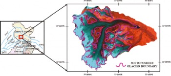
Fig. 1. Samudratapu glacier located in the Chenab basin, Himachal Himalaya. AWiFS image (false-colour composite with band combination, red: B4, green: B3, blue: B2) of the Samudratapu watershed overlaid by the boundary of the glacier digitized from Survey of India topographic maps of 1963.
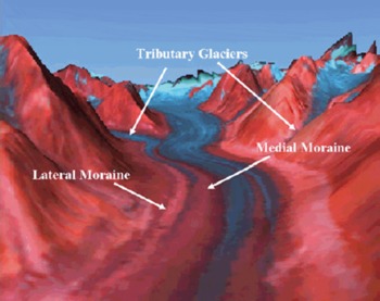
Fig. 2. Perspective view of Samudratapu glacier from Terra ASTER image (false-colour composite with band combination, red: B5, green: B3, blue: B2) draped over a DEM of the area, showing the confluence of tributary glaciers with the main glacier and moraine cover.
Data
Topographic maps at scale 1 : 50 000, surveyed by Survey of India (SOI) in 1963, were used to georeference the remote-sensing data and to generate a digital elevation model (DEM). Topographic maps were also used to create a mask corresponding to the glacier area.
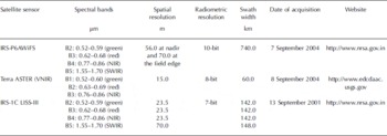
Remote-sensing data from the IRS-P6 Advanced Wide Field Sensor (AWiFS), IRS-1C LISS-III and the Terra ASTER sensor were used (Table 1). Images for the post-monsoon season (August and September) were selected because during this period the temporary snow cover is at its minimum and all the glacier zones can be clearly demarcated. An ASTER visible/near-infrared (VNIR) image was used as a reference datum for assessing the accuracy of glacier-cover maps, for two reasons: its high spatial resolution (Table 1), and its low temporal difference (1 day) with reference to the AWiFS image. Remote-sensing data from IRS LISS-III and IRS AWiFS provide a temporal difference of 3 years for the study of temporal changes, particularly debris cover. Images from the same month were selected to eliminate seasonal changes in the areal extents of various classes.
Table 1. Specifications of remote-sensing data used in the study
For optimum classification of image objects, it is preferred that the data are expressed in physical units, such as reflectance. As different objects having the same DN values may have differences in spectral reflectance, the use of quantitative spectral reflectance values may improve discrimination between objects. In this work, remote-sensing data have first been converted into topographically corrected reflectance data. Correction of the data for topographic variation requires terrain parameters such as slope and aspect. These input parameters were derived from a DEM created through digitization of contours on SOI topographical maps (scale: 1 : 50 000).
Methodology
The methodology comprises georeferencing of remote-sensing images with topographical maps, computation of topographically corrected reflectance at each pixel of the remote-sensing image and supervised classification of the reflectance data for mapping of six land-cover classes: debris, snow, ice, MID, water, and valley rock. Figure 3 shows the schematic representation of the broad methodology adopted.
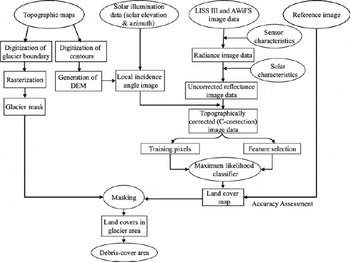
Fig. 3. Schematic data flow of methodology adopted.
Computation of topographically corrected reflectance
Sensors on board various satellites measure the upwelling radiance above the Earth’s atmosphere, and represent the received signals as digital numbers, which depend on calibration parameters of the sensor. Radiance reaching the sensor depends upon the target reflectance and the solar irradiance on the target. Reflectance is the ratio of upwelling radiation from the surface to the solar radiation incident on the surface. The magnitude of solar irradiance impinging on a sloping surface greatly depends on the orientation of the target surface. Thus, in a rugged terrain with highly undulating surfaces and steep slopes such as the Himalaya, the reflected radiance reaching the sensor is profoundly influenced by the orientation (slope and aspect) of the target surface. Therefore, for optimum detection/mapping of various target classes, an analysis based on DN values may not be appropriate, since these values inherently include radiometric variations arising from topography, sensor calibration, etc. Hence, the DN values have to be converted into topographically corrected reflectance data.
The variations in remote-sensing reflectance image data due to topography can be adjusted using either of two methods: a method based on image ratioing or a method based on local illumination geometry. The image ratio approach is a simple one, with the assumption that the effect of topography is spectrally uniform and is valid for all incidence angles; however, a major disadvantage of the method is that the radiometric resolution of the image tends to decrease since ratio images are quite noisy compared to the original data.
The second method is based on illumination modelling and requires a DEM of the area at the same spatial resolution as that of the image, for computing the local incidence angle, i. Several methods of topographic correction based on illumination modelling have been developed (e.g. cosine correction, Minnaert correction, statistical–empirical methods, C-correction (Reference Teillet, Guindon and GoodenoughTeillet and others, 1982; Reference TeilletTeillet, 1986; Reference Meyer, Itten, Kellenberger, Sandmeier and SandmeierMeyer and others, 1993)). The bidirectional reflectance distribution function (BRDF) requires definition of surface reflectance characteristics for all possible angle combinations of incidence and reflection, and its use may be the best for topographic correction (Reference Sandmeier and IttenSandmeier and Itten, 1997; Reference Nolin and DozierNolin and Dozier, 2000). However, owing to various difficulties in computing the BRDF for field-based problems, more general and approximate approaches are used. Previous studies (e.g. Reference Meyer, Itten, Kellenberger, Sandmeier and SandmeierMeyer and others, 1993) indicate that the C-correction method is suitable. It has therefore been used in the present work for topographic normalization. For a detailed description of procedure for C-correction, see Reference Teillet, Guindon and GoodenoughTeillet and others (1982), Reference TeilletTeillet, (1986), Reference Meyer, Itten, Kellenberger, Sandmeier and SandmeierMeyer and others (1993) and Reference Gupta, Ghosh and HaritashyaGupta and others (2007).
Supervised classification of reflectance data
The topographically corrected reflectance data were subjected to supervised classification. The aim of digital image classification was to produce thematic maps where each pixel in the image is assigned to a class or a theme on the basis of spectral response at each pixel. There are two basic approaches to digital image classification: supervised or unsupervised (Reference Richards and JiaRichards and Jia, 1999). Both have been used widely for snow and glacier mapping (Reference Aniya, Sato, Naruse, Skvarca and CasassaAniya and others, 1996; Reference Bronge and BrongeBronge and Bronge, 1999; Reference Sidjak and WheateSidjak and Wheate, 1999; Reference Slater, Slogett, Rees and SteelSlater and others, 1999).
Various standard stages of a supervised image classification have been followed: training, feature selection, allocation and testing (Reference Arora and FoodyArora and Foody, 1997). Figure 4 shows the typical reflectance curves of the various land-cover classes of interest. Training areas for all the six classes were selected interactively on the image itself. The total number of training pixels (2631 pixels for the LISS-III image and 915 pixels for the AWiFS image) comprises about 1% of the total number of pixels in the images. Feature selection was performed to quantitatively select that subset of bands (i.e. features) which provides the highest degree of separability between classes to be mapped using transformed divergence (TD) (Reference MatherMather, 2004). TD is a derivative of simple divergence and its values may range from 0 to 2000 (Reference JensenJensen, 1996). A TD value of 2000 indicates the highest separability, and values below 1700 indicate low separability.
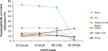
Fig. 4. Typical spectral reflectance curves for the various land-cover classes in the glacier terrain.
The separability analysis shows that the three-band combination B2, B4, B5 produces the highest TD values for both AWiFS and LISS-III data. Therefore this band combination was used for classification with a maximum likelihood classifier (MLC). MLC allocates each pixel to the class of which it has the highest probability of membership. Detailed description of this classifier may be found in various works (e.g. Reference Richards and JiaRichards and Jia, 1999). The land-cover maps resulting from the MLC are masked with the glacier mask in order to yield glacier-cover maps showing the distribution of the six classes in the glacier area (Fig. 5).
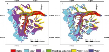
Fig. 5. Glacier-cover maps from (a) AWiFS and (b) LISS-III image data. The brown-coloured ellipses show a marked increase in the debris cover over the glacier from 2001 to 2004 (see text).
Classification accuracy assessment
The accuracy of the classified maps was assessed using error-matrix based accuracy measures (Reference CongaltonCongalton, 1991). An ASTER digital image (VNIR spatial resolution 15 m) was selected as reference data for assessing the accuracy of the image classification. The number of testing pixels collected in equalized random fashion in the case of AWiFS-derived maps is 100 pixels per class. For LISS-III data, it is 200 pixels per class. The error matrix can be utilized to determine the over-all accuracy of the map and individual class accuracies in the form of user’s and producer’s accuracies (Reference CongaltonCongalton, 1991). The overall accuracy is used to indicate the accuracy of the whole classification (i.e. the number of correctly classified pixels divided by the total number of testing pixels). The producer’s accuracy relates to the probability that a reference sample was correctly mapped, and measures the omission error. The user’s accuracy indicates the probability that a sample from the land-cover map actually matches what it was in the reference data, and measures the commission error.
The error-matrix based accuracy assessment reveals that the methodology applied here has been quite successful in mapping the debris cover and other land-cover classes. Overall accuracies of glacier-cover maps derived from AWiFS and LISS-III data are found to be 83.7% and 89.1% respectively. The relatively high value of overall accuracy for the glacier-cover map obtained from LISS-III image data may be attributed to higher spatial resolution of LISS-III data compared to AWiFS data.
Since the focus of this study is on developing a simple yet effective method for accurate estimation of the debris cover over glaciers, the individual class accuracies have also been examined. The error-matrix based producer’s and user’s accuracy values for all the six classes are given in Table 2. The producer’s and user’s debris-cover accuracy using both the datasets are found to be in the ranges 76–82% and 82–95% respectively. This sufficiently implies that supervised classification of topographically corrected reflectance data is fairly effective for the extraction of debris cover.
Table 2. Producer’s and user’s accuracies (%) (Reference CongaltonCongalton, 1991) of six land-cover classes in glacier-cover maps derived from AWiFS and LISS-III data of the area

However, a careful study and analysis of the error matrix shown in Table 3 reveals that errors of omission and commission are mostly found among four land-cover classes: MID, debris, valley rock, and water. This is largely due to spectral similarity between these classes, which is a major impediment in their precise discrimination. In summary, it can be stated that although the method proposed here is able to map the debris cover with sufficiently high accuracy, there is scope for further improvement through approaches such as multisource and sub-pixel classification (Reference Srinivasan and RichardsSrinivasan and Richards, 1990; Reference Arora and FoodyArora and Foody, 1997; Reference Binaghi, Madella, Montesano and RampiniBinaghi and others, 1997; Reference AroraArora, 1999; Reference Arora and MathurArora and Mathur, 2001).
Table 3. Error matrix (values in %) for the glacier-cover map produced from AWiFS data

Change Detection
Deglaciation and recession of the glacier
An intercomparative study of the maps generated from the supervised classification of the remote-sensing data and also the glacier mask created from the SOI toposheets has also been carried out to assess the trends of glacier depletion and recession in the region (Fig. 6).
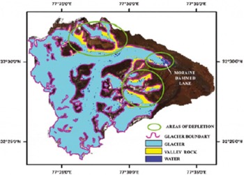
Fig. 6. Comparative assessment of the glacier area obtained from AWiFS (2004) and the glacier boundary derived from SOI toposheets (1963). The false-colour composite (red: B4, green: B3, blue: B2) is from the AWiFS image. All the glacier-cover classes (snow, ice, MID, debris) have been merged into a single class: glacier. Note the presence of valley-rock and water within the glacier area, indicating glacier depletion and recession (circled in green).
The presence of valley rock within the glacier area provides evidence of deglaciation and indicates that these areas have been vacated by the glacier, evidently as a result of regional climatic changes. Similarly, the remote-sensing data show the presence of water in the snout region, which actually is a moraine-dammed lake at the terminus of this glacier. However, the SOI toposheets (1963) show this area as a part of the glacier. Thus, apparently, due to the recession of the glacier and accompanied melting a moraine-dammed lake has developed at the snout.
The recession and depletion of the glacier has also been estimated quantitatively (Table 4). The glacier area is found to be 110.5 km2 in 1963, decreasing to 101.7 km2 in 2001, and then further to 96.8 km2 by 2004. A detailed study has also been made of the change in glacier snout location (Fig. 7). It is observed that the glacier has receded by 587.7 m (15.5 m a−1) from 1963 to 2001 and by about 168.6 m (56 m a−1) from 2001 to 2004. This is a total retreat of 756.3 m from 1963 to 2004. The increased rate of glacier recession in recent years (2001–04) is considerable and the data conform with the reported accelerated rate of overall glacier depletion (Reference Dobhal, Gergan and ThayyenDobhal and others, 2004; Reference Kulkarni, Rathore, Mahajan and MathurKulkarni and others, 2005, Reference Kulkarni2007) and appear to be a result of change in the regional climate.
Table 4. Quantitative estimates of glacier depletion for 1976–2001 and 2001–04, from SOI toposheets (1963), LISS-III image (2001) and AWiFS image (2004)
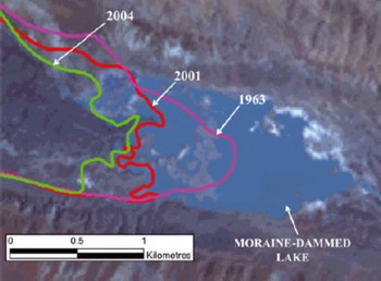
Fig. 7. Change detection of glacier snout. The position of the glacier snout was mapped in 1963 (SOI toposheets), 2001 (IRS-1C LISS-III image) and 2004 (IRS-P6 AWiFS image)
Temporal variation of debris cover
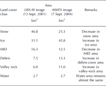
Intercomparison of the areal estimates of various land-cover classes (debris, snow, ice, MID, water, and valley rock) from the glacier-cover maps obtained from LISS-III (13 September 2001) and AWiFS (7 September 2004) images (Table 5) shows some interesting trends. As stated earlier, remote-sensing data from the same month were chosen to minimize the effect of seasonal changes in areal estimates.
The results in Table 5 show that in a span of 3 years (2001–04), the area of debris cover increased by 76.5% from 7.5 km2 to 13.3 km2. This increase can also be observed clearly in the glacier-cover maps (Fig. 5; areas denoted by brown ellipses). Assessment of such a change in the areal extent of debris cover over glaciers is valuable, as debris cover is not only considered a sensitive indicator of glacier health but also influences the process of glacier melting. Besides debris cover, the areal extents of other classes are also found to vary. The areas of snow cover and MID have decreased, with an accompanying increase in the areas of ice, debris and valley rock. All these changes appear to be intimately linked with the general climatological warming, increased rates of ablation, depletion and recession. Similarly, the MID-covered area has decreased due to melting, leading to an increase in the area covered by debris. Also, the shrinking of the glacier has resulted in an increase in valley rock area. Thus, accelerated rates of recession, overall glacier depletion, and increase in debris cover, as deduced by analysis of remote-sensing data, provide strong evidence of overall degeneration and wasting of the glacier. All these facts again point towards the urgent need for regular monitoring of various glacier land-cover classes, particularly debris cover.
Table 5. Comparison of the areal estimates of various land-cover classes from classified glacier-cover maps derived from LISS-III and AWiFS data of the area
Concluding Remarks
It is very important to map debris cover over glaciers since it is known to influence the rate of glacier melting to a large extent and is considered an important parameter of glacier health. In this study, supervised classification of topographically corrected optical remote-sensing data (IRS-1C LISS-III and IRS-P6 AWiFS) was carried out in a small part of the Chenab basin. Terra ASTER VNIR data were used as reference data for accuracy assessment. Based on the analysis of results from this study, the following conclusions can be drawn:
-
1. In this glacier terrain, there are six different land-cover types as characterized by the spectral reflectance data: snow, ice, MID, debris, valley rock, and water. The separability analysis shows that the band combination B2, B4, B5 has the highest value of transformed divergence for the two remote-sensing images (IRS-1C LISS-III and IRS-P6 AWiFS), indicating maximum separability between the land-cover classes selected.
-
2. Overall accuracies of classification of remote-sensing images via maximum likelihood classification are found to range from 83.7% to 89.1%, whereas the individual accuracy of debris-cover class can be mapped with accuracy ranging from 82% to 95%. This shows that the supervised classification of topographically corrected reflectance data is effective for the extraction of debris cover from remote-sensing data.
-
3. Comparison of the total glacier-cover area obtained from the SOI topographic maps (1963) and the recent satellite remote-sensing data (2001 and 2004) reveals that the glacier area has reduced from 110.5 km2 in 1963 to 101.7 km2 in 2001, and further to 96.8 km2 in 2004. This amounts to an overall deglaciation of 13.7 km2 during the past 41 years.
-
4. The glacier snout position was found to have retreated by 587.7 m (15.5 m a−1) from 1963 to 2001 and by about 168.6 m (56 m a−1) from 2001 to 2004. Thus in the past 41 years (1963–2004) the glacier has receded by about 756 m.
-
5. The recent glacier retreat and depletion is found to be accompanied by a marked increase in the extent of debris cover, which has increased by almost 76.5% in a span of just 3 years (from 7.5 km2 in 2001 to 13.3 km2 in 2004). An increase in valley-rock area is also found during this (2001–04) period.
-
6. Therefore, the accelerated rates of recession and overall glacier depletion observed for the recent years 2001–04, together with the marked increase in debris cover, may be interpreted as strong indicators of the overall degeneration and wasting of the glacier.
The study sufficiently demonstrates the applicability of the remote-sensing data in monitoring glacier terrain, and particularly mapping debris-cover area.
Acknowledgements
A. Shukla thanks the Council of Scientific and industrial Research (CSIR), India, for providing a research fellowship. We thank two reviewers for valuable comments on an earlier version of the manuscript.


