
Optimizing Sensors Locations for Tsunami Warning System
Volume 7, Issue 6, Page No 256-261, 2022
Author’s Name: Mikhail Lavrentiev1,a), Dmitry Kuzakov1, Andrey Marchuk1,2
View Affiliations
1Institute of Automation and Electrometry SB RAS, Novosibirsk, 630090, Russia
2Institute of Computational Mathematics and Mathematical Geophysics SB RAS, Novosibirsk, 630090, Russia
a)whom correspondence should be addressed. E-mail: mmlavrentiev@gmail.com
Adv. Sci. Technol. Eng. Syst. J. 7(6), 256-261 (2022); ![]() DOI: 10.25046/aj070629
DOI: 10.25046/aj070629
Keywords: Initial sea surface displacement, Tsunami source parameters, Part of wave profile

Export Citations
To reduce the time necessary for determination of tsunami source parameters it is proposed to optimize the location of sensors system and to use only a part of the measured wave profile. Based on computation, it is possible to balance the number of sensors in use and the time period after the earthquake needed to obtain tsunami wave parameters. Numerical experiments show that even a part of the wave period (compared to ¼ of the entire period) provides enough information to get the wave amplitude within the well-known concept of calculation in advance. This is due to the application of Fourier theory in the form of orthogonal decomposition of the measured wave profile. It is important that the proposed algorithm requires only a few seconds using regular personal computer. Using the real depth profile offshore Japan we compute the time required to calculate the wave amplitude (with 10 percent accuracy) in case of one, two and three sensors. Optimization could be performed in terms of minimal time required to get the wave profile. It is also possible to calculate the sensor network design, which provides the maximal time between wave parameters determination and the wave approaching nearest coast. The new feature here observed is that optimal positions of sensors are different if one needs minimizing time to detect tsunami wave or maximazing time it takes the wave to approach the nearest cost after recovering the wave parameters at source. This may require to rearrange decision making at tsunami warning centers.
Received: 06 August 2022, Accepted: 08 December 2022, Published Online: 20 December 2022
1. Introduction
This paper is an extension of the work originally presented in the conference OCEANS 2021: San Diego – Porto [1].
As a rule, the numerical modeling modulus of tsunami warning system should contain the following three major parts: wave generation (earthquake magnitude and hypocenter location recalculated in terms of the initial seabed displacement), wave propagation and inundation of the dry land. For example, our reference code, the MOST (Method of Splitting Tsunami) software package (see [2,3]), has all these parts. Alternative codes have similar structure [4,5]. It is natural to use “initial disturbance” at tsunami source as the “input data” to calculate tsunami wave propagation from the source to the coastal area. Displacement of the sea bed (due to the earthquake) could be evaluated on the basis of knowledge of the Earth crust structure and the location of the earthquake epicenter. So, regardless the underlying reasons, in any case the so-obtained initial displacement is nothing but approximation. We propose to use instead the sea surface displacement at tsunami source, obtained by processing the measured profile of the real tsunami wave. These measured data are available due to the rather well-developed system of bottom pressure sensors, located at sea bed around Pacific Ocean, given in Figure 1 from [6].
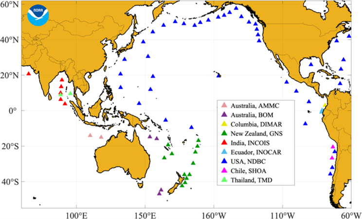
Figure 1: Location of Dart buoys around the Pacific Ocean [6]
In addition, there exist systems of bottom sensors, connected to the dry lend (processing centers) by a cable, for example DONET (Dense Oceanfloor Network system for Earthquakes and Tsunamis) [7] and S-net (Seafloor observation network for earthquakes and tsunamis) [8] being developed in Japan. Figure 2, taken from [8], shows the location of S-net deep-water stations eastward of Honshu Is.
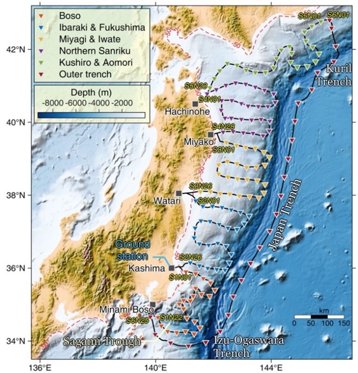
Figure 2: Configuration of the S-net observation system along the Japan trench [8]
In some publications, the optimal positioning of the sensor network refers to the location of sensors that allow detection of a tsunami wave in the shortest time after its occurrence (see, for example, [9] and the references therein). The present article, however, deals with the configuration of a network of deep-water recorders, not for the earliest detection of the tsunami occurrence, but for determining the water surface displacement profile with the required accuracy in the shortest possible time.
In [10] the S-net observation data are used reconstruct the source parameters by the sequential multiple linear regression method.
The original idea of calculation in advance was used in [11]. It consists in introduction of so-called Unit Sources (UnSs). These are nothing but rectangles 50×100 km – typical size of the sea bed displacement in case of 7.5 M earthquake. It is possible to simulate numerically tsunami wave propagation initiated by a given displacement form. Covering the particular subduction zone with such UnSs (along with the typical for this zone shape of the initial sea bed displacement) one can create “in advance” the database of the calculated tsunami wave time series (synthetic mareograms). Suppose that we have a sea bottom pressure sensor (a number of those are installed over the Pacific Ocean) which is able to report the parameters of the tsunami wave passing over in a real time mode. Having such a measured wave profile we now approximate it as a linear combination of several calculated wave profiles, each being initiated by one of the UnSs [12]. In fact, such a database exists and is available for use. System of UnSs covers major subduction zones around Pacific Ocean [13].
As was noted in [14], even a part of the measured wave profile is enough to reconstruct the main tsunami wave parameters within the calculation in advance strategy. We believe that 10% error is acceptable to decide if a particular wave is dangerous in a given location. Here we show how the necessary time to determine the wave amplitude at source depends of the number of sensors one uses. This is done by the example of three different locations of the “composed” tsunami source within a particular water area offshore Japan.
The rest of this paper is composed as follows. We first describe the “calculation in advance” data inversion strategy. Then the idea of orthogonal decomposition method is given. The method has a very low computational cost and makes it possible to obtain an approximation of tsunami source parameters by using only a part of the measured wave profile. Digital bathymetry offshore the central part of Honshu Island (Japan) is then introduced. Setting up of numerical experiments is then described, including location of model tsunami sources and artificial water level measurement sensors. The obtained numerical results are given in Section 3. Finally, these results are briefly discussed.
2. Setup of Numerical Experiments
2.1. Problem Statement
As part of the general problem of estimating the tsunami hazard in the shortest possible time, let us determine the role of the location of the system of deep-water sensors. We will assume that, at the cost of allowing 10% error in obtained wave amplitude, the source parameters are determined from data from a single sensor, the first one the wave has reached. Moreover, we will use only part of the wave period, which is about 1/4 of this first period (having the positive phase first). The exact value of this NPWP (Necessary Part of Wave Period) is determined automatically, on the basis that the amplitude values practically stop growing as the wave passes over the sensor [14]. Let us consider the ratio of the number of sensors to the time required to determine the approximate values of the wave parameters in the tsunami source.
Following [3], we will assume that the epicenter of the earthquake is located within a certain zone (subduction zone). This assumed zone is covered by 8 rectangles of size 50×100 km – the typical size of the seafloor deformation zone during an earthquake of magnitude M=7.5 (the accepted threshold value of magnitude for the formation of tsunami waves). In each of these rectangles (Unit Sources – UnSs) is placed a perturbation with a shape characteristic of seafloor deformation resulting from earthquakes in this subduction zone. The seafloor deformation during a stronger earthquake will be approximated by a linear combination of four of these UnSs with some coefficients. The problem of determining the source parameters comes down to determining the set of these amplification coefficients.
2.2. Orthogonal Decomposition Method
To elaborate a fast and robust algorithm for the determination of the above amplification coefficients, Fourier series theory was used, as it deals in particular with optimal approximation of a given function with the linear combination of functions being orthogonal and normalized.
Let f(t) be the measured time series of the wave profile (marigram). One can consider the data from DART buoy or nay alternative sensor. By , k=1,…,n, let us denote the calculated wave profiles, obtained (by direct numerical solutions to the linear or nonlinear shallow water system [15]) at the same point of sensor location. The parameter k means that the source of this wave is located at the k-th UnS having “standard” shape. As was shown numerically, these functions, , could be considered linearly independent. To describe better the measured wave, one should determine the coefficients, bk, for the linear combination of these functions, for which the below difference in L2 norm is the smallest:
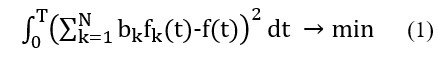
In such a statement the problem of determination of the wave parameters at source is reduced to the one of the optimal approximation of a given function f(t) by the linear combination of functions {fk(t)}.
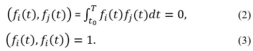
The Fourier series theory states that the coefficients of such optimal approximation (1) are exactly the Fourier coefficients of expansion of f(t) in a series with respect to {fk(t)} (see, for example, [16]), provided that the system {fk(t)} is orthogonal and normalized:
So, the Fourier series theory was used in [17] to design the algorithm to determine coefficients for optimal approximation of the measured tsunami wave. This algorithm, tested in [1,14,18], consists of several stages.
At the first stage the “marigrams” {fk(t)} obtained from the unit sources should be recalculated to meet the requirements (2)-(3).
Then, the function f(t) (tsunami wave profile) should be expanded to the Fourier series with respect to recalculated synthetic marigrams. At the last stage the obtained Fourier coefficients are transformed into the sought coefficients in (1).
Note that the described algorithm has a very low computational cost as mostly simple algebraic operations are involved. We consider calculation of integrals (scalar products and L2 norms as simple operations, too.) During the performed numerical experiments it takes less than a second using regular personal computer.
2.3. Domain for Numerical Study – Bathymetry
All numerical studies were arranged at the water area offshore Kanto Region, central part of the Honshu Island (Japan). JODC database (see [19]) was used to create the gridded bathymetry for the computation area, given in Figure 3. The area under study is bounded in East-West direction by 137.0º and 143.0º East Longitude, and in North-South direction by 32.0º and 37.0º North Latitude. Spatial grid steps are 223 m (East-West direction) and 273 m (North-South direction. Array of computational nodes has size of 2000×2500.
2.4. Description of Numerical Studies Setup
Tsunami sources in subduction zones usually extend along deep-water troughs. In this case, the source is most effectively reconstructed by sensors located in the direction of the short axis of such sources. In the area under consideration the deep-water trench is oriented from North to South (Figure 3), so the possible sources are extended in this direction, and the virtual sensors are located along the meridian, which, in our opinion, allows reconstructing effectively the initial displacement of the water surface using the data of a minimum number of sensors. Along the northeastern coast of Honshu Island, where S-net sensors are installed (Figure 2), the possible tsunami sources are extended in the direction of Japan Trench, which allows an optimal choice among the already available deep-water recorders. This is not yet possible in the area of the Kanto Peninsula.
We consider offshore water area at the Izu-Bonin subduction zone. Suppose that tsunami sources are expected within the strip covered by eight UnSs (having size 50×100 km each), indicated as white rectangles, see the Figure 1. In total the 100×400 km zone is considered. Simulating a rather strong earthquake, the Composed Sources (CSs) are studied. These are nothing but linear combinations of four neighboring USs with certain amplification coefficients. We choose the following values for the coefficients (0.7, 0.8, 1.2, 1.3). It means that for each of the CSi, i=1,2,3, (indicated in Figure 3) the upper-left UnS has the coefficient 0.7 (in the linear combination, which determines our Composed Source), the lower-left – 0.8, upper-right – 1.2 and lower-right – 1.3. The amplitude of sea surface indignation of each of these CSi does not exceed +150 cm and its shape is given in Figure 4. Form of such a CS is typical in the area of study. Our task is to determine these amplification coefficients.
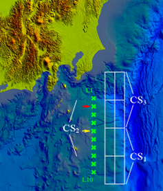
Figure 3: Digital bathymetry of water area under study. Artificial tsunami sources are indicated as CSi. Green crosses indicate artificial sensors
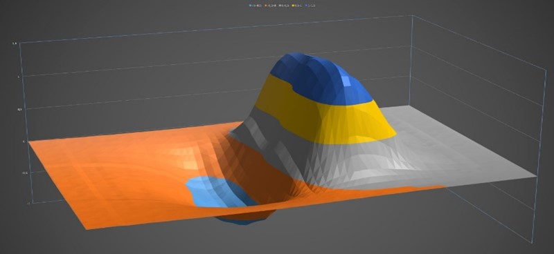
Figure 4: Visualization of CSi – water level in the artificially composed tsunami source having size 100 x 200 km
A number of virtual tsunami detection sensors are located close to the subduction zone. Exact positions of these 10 “tsunameters” are indicated by green crosses. Numbering is arranged from up (sensor L1) to down, the “last one is indicated as L10. These “virtual tsunameters” Li could coincide with the existing sensors from S-net and DONET, the other could suggest possible positions of DART buoys.
3. Numerical Results
A series of numerical calculations of tsunami propagation from each of the 8 UnSs under consideration was performed to obtain synthetic tsunami profiles, on the basis of which the source parameters recovery algorithm was constructed. For numerical modeling, the MOST algorithm [2,3], which correctly describes tsunami propagation in a sufficiently deep-water area, was used. This method uses difference scheme based on spatial direction splitting difference scheme to approximate the system of nonlinear shallow water differential equations. Calculations can result in wave series at all 10 tsunami recorder locations from each UnS.
A series of computational experiments were carried out to assess the efficiency of reconstructing a composed sources CSi, i=1,2,3, by using the data from deep-water recorders located at different points in the region. The gridded bathymetry for these calculations is described in Section 2.2, and the field of water surface displacement in the basis (Unit) Source, constructed using the seismic source model in elastic half-space [12], is presented in Figure 5.
Based on the results of numerical modeling of tsunami propagation generated by each of 8 such UnSs, a database of synthetic mareograms (wave time series) at the locations of 10 virtual deep-water detectors (given in Figure 3) was created. Wave series calculated at these virtual tsunameters location were used to reconstruct the source composed of 4 UnSs with different amplification coefficients. To estimate the quality of restoration of composed sources CSi, i=1,2,3, the results of tsunami modeling generated by each CSi at different sensors were used. The time needed for recovery and deviation estimate from the exact wave profile were determined and are presented in the form of tables.
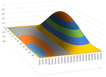
Figure 5. Water surface displacement in the Unit Source having size 50 x 100 km
Results of numerical simulation described in [14] are given in Tables 1-3 below.
The following “critical” time designations are used in the tables:
NPWP – necessary part of the wave profile, measured in seconds, to determine correctly (within 10% error) the coefficients in approximation (1);
T1 (sec) – time moment in which the wave first maximum appears at the given virtual sensor;
T2 (sec) – the time it takes the wave to approach the nearest coast after the moment where the coefficients in (1) are correctly determined.
Table 1: Source CS1 (see Figure 1). Wave travel time to the nearest coast is equal to 1260 sec.
| No Rec. | NPWP, sec. | T1, sec | T2, sec |
| L1 | 1031 | 740 | 229 |
| L2 | 794 | 630 | 466 |
| L3 | 697 | 525 | 563 |
| L4 | 552 | 435 | 708 |
| L5 | 478 | 375 | 782 |
| L6 | 469 | 358 | 791 |
| L7 | 383 | 367 | 877 |
| L8 | 385 | 372 | 875 |
| L9 | 348 | 336 | 912 |
| L10 | 317 | 306 | 943 |
Table 2: Source CS2 (Figure 1, the middle one). Wave travel time to the nearest coast is equal to 886 sec.
| No Rec. | NPWP, sec. | T1, sec | T2, sec |
| L1 | 443 | 343 | 443 |
| L2 | 358 | 285 | 528 |
| L3 | 262 | 266 | 624 |
| L4 | 319 | 303 | 567 |
| L5 | 354 | 340 | 532 |
| L6 | 389 | 373 | 497 |
| L7 | 382 | 368 | 504 |
| L8 | 473 | 366 | 413 |
| L9 | 502 | 391 | 384 |
| L10 | 550 | 443 | 336 |
Let us consider three scenarios of a possible tsunami. The combined sources of the form shown in Figure 4 have three possible positions CSi (i=1,2,3), see Figure 3. The analysis of Tables 1-3 shows that if we have only one working sensor at our disposal, it should be placed at point L5 (yellow arrow in Figure 1). The guaranteed detection time of the source parameters will be 478 seconds (case of CS3 source). In the case of any other location of the sensor in at least one scenario under consideration, this time will be longer. However, if we want to have the longest time available before the wave arrives on shore after determining the source parameters, we should choose sensor position L2 (red arrow in Figure 3). This time will be 466 sec (again for the source CS3). With a different location of the sensor, we will find a case where this time will be shorter.
If we have two sensors at our disposal, they must be chosen differently. For the fastest detection time of the source parameters in the “worst” of three cases it will be sensors L3 and L10 (shown by yellow arrows in Figure 6), and this time will be 317 seconds (source CS3). That is, the addition of one sensor allows reducing the required time by almost 1.5 times. If we want to achieve the longest possible time before the wave arrives on the shore, we should place the sensors at the points L1 and L4 (shown by red arrows in Figure 6). This time will be 488 seconds (source CS1), which is slightly longer than in the case of one sensor.
Table 3: Source CS3 (the upper one at Figure 1). Wave travel time to the nearest coast is equal to 719 sec.
| No Rec. | NPWP, sec. | T1, sec | T2, sec |
| L1 | 231 | 218 | 488 |
| L2 | 242 | 233 | 477 |
| L3 | 296 | 284 | 423 |
| L4 | 314 | 304 | 405 |
| L5 | 394 | 333 | 325 |
| L6 | 500 | 412 | 219 |
| L7 | 626 | 503 | 93 |
| L8 | 782 | 615 | 0 |
| L9 | 935 | 740 | 0 |
| L10 | 1049 | 849 | 0 |
For the convenience of further analysis, the data about the optimal location of one and two sensors are collected in Tables 4 and 5.
Table 4: Optimal location of 1 and 2 sensors for fastest determination of source parameters
| Source parameters detected, sec | |||
| CS1 | CS2 | CS3 | |
| L5 | 394 | 354 | 478 |
| L3+L10 | 296 | 262 | 317 |
It is clear from Table 4 that by introducing an additional sensor to the monitoring system it is possible to reduce the time for source parameters determination. The “reduction rate” for the necessary time is similar for all considered scenarios CSi, i=1,2,3. We may assume that doubling the number of sensors leads to the reduction of time to detect the source parameters compared to 30-40%. Additional numerical experiments are needed to get the exact numbers, which should definitely depend on a particular subduction zone.
Table 5: Optimal location of 1 and 2 sensors to have larger travelling time for the wave to approach nearest dry land after source parameters determination
| Wave travelling time to approach dry land after coefficients determination, sec | |||
| CS1 | CS2 | CS3 | |
| L2 | 477 | 528 | 466 |
| L1+L4 | 488 | 567 | 708 |
In case we are interested in time one has after obtaining the source parameters before the wave approaches nearest shore, Table 5 shows, that this time increases after taking into consideration an additional sensor. However, the observed gain is practically negligible for CS1 scenario and is compared to 40 sec (about 8%) for CS2 scenario. Note that in these two scenarios we are able to determine source parameters rather fast, see Table 4.
In case of the most unfavorable CS3 with the largest time required for the source parameters determination, wave traveling time to the nearest dry land increases valuably according to Table 5. This fact leads to a conclusion, that it is far nontrivial to choose the optimality criteria for the monitoring system.
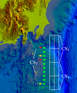
Figure 6: Visualization of the digital bathymetry. Model Composed tsunami sources are indicated as CSi. Green crosses indicate artificial sensors
4. Discussion
Most studies on the organization of the tsunami detection system (location of sensors) to provide data to tsunami warning services have the objective of determining the wave parameters at the source as quickly as possible. By doing so, the distribution of maximum wave heights along the coastline can be predicted more quickly. However, numerical results show that a different location of the sensors would provide more time before the wave arrives at the nearest shore. Considering the fairly densely populated coastline of Japan, this parameter seems to be at least as important as the fastest wave detection. This should be taken into account when planning the location of additional sensors.
The optimal location of the surveillance system can be calculated (not just being randomly suggested) according to the selected criterion. The more sensors are used, the better the value of the selected criterion will be – the source parameters will be determined faster or after determining the source parameters there will be more time until the wave reaches the nearest shore.
Thus, when switching from one to two sensors in the model case under consideration, the time for which the algorithm determines the source parameters decreases from 478 to 317 sec (Table 4), that is, practically one and a half times (source CS3). Let us note that in other considered scenarios as well (sources CS1 and CS2) this time decreases from 394 to 296 sec (1.33 times less time needed) for the CS1 case and from 354 to 262 sec (1.35 times less) for the CS2 source.
For the criterion “maximum time remaining until the wave reaches the nearest shore”, this time increases from 466 to 488 sec when an additional sensor is added (Table 4). This is a comparative increase, but for the CS3 source scenario, the increase in time to analyze and make decisions to evacuate the population is 242 sec (from 466 to 708 sec). This certainly may save lives.
Thus, when designing a monitoring system for tsunami warning centers, it is advisable to choose a criterion for the optimality of the system, taking into account various factors (including the cost of creation) and to optimize the location of sensors.
Conflict of Interest
The authors declare no conflict of interest.
Acknowledgment
This research was carried out under state contract with IAE SB RAS (121041800012-8) and with ICMMG SB RAS (0315-2019-0004) and under state contract with ICMMG SB RAS (0315-2019-0004).
- D. Kuzakov, M. Lavrentiev, An. Marchuk, “Toward the optimization of measurement system for tsunami warning,” in 2021 International Conference Global Oceans 2021: San Diego – Porto, In Person Virtual, September 20-23, 2021, Town and County San Diego, doi: 10.23919/OCEANS44145.2021.9705912
- V.V. Titov, F.I. Gonzalez, “Implementation and testing of the method of splitting tsunami (MOST) model,” in NOAA Technical Memorandum ERL PMEL-112, USA,1977.
- E. Gica, M. Spillane, V.V. Titov, C.D. Chamberlin, J.C. Newman, “Development of the forecast propagation database for NOAA’s Short-term Inundation Forecast for Tsunamis (SIFT),” in NOAA Tech. Memo. OAR PMEL-139, NTIS: PB2008-109391, 2008.
- X. Wang, W.L. Power, COMCOT: A Tsunami Generation Propagation and Run-Up Model, GNS Science, 2011.
- A.C. Yalciner, B. Alpar, Y. Altinok, I. Ozbay, F. Imamura, “Tsunamis in the Sea of Marmara: Historical Documents for the Past, Models for Future,” Marine Geology, 190, 445-463, 2002.
- DART (Deep-ocean Assessment and Reporting of Tsunamis). Available online: URL http://nctr.pmel.noaa.gov/Dart/ (accessed on 20.07.2022).
- DONET system concept. Available online: URL https://www.jamstec.go.jp/donet/e/ (accessed on 31.07.2022).
- I.E. Mulia, K. Satake, “Synthetic analysis of the efficacy of the S-net system in tsunami forecasting,” Earth Planets Space 73(36), 2021. https://doi.org/10.1186/s40623-021-01368-6
- A. Ferrolino, R. Mendoza, I. Magdalena, J.E. Lope, “Application of particle swarm optimization in optimal placement of tsunami sensors,” Peer J Comput. Sci. 6:e333, 2020. DOI 10.7717/peerj-cs.333
- L. Yao, K. Goda, “Hazard and Risk-Based Tsunami Early Warning Algorithms for Ocean Bottom Sensor S-Net System in Tohoku, Japan, Using Sequential Multiple Linear Regression,” Geosciences 12.9: 350, 2022.
- D.B. Percival, D.W. Denbo, M.C. Eble, E. Gica, H.O. Mofjeld, M.C. Spillane, L. Tang, V.V. Titov, “Extraction of tsunami source coefficients via inversion of DART® buoy data,” Nat. Hazards, 58(1), 567–590, 2011, doi: 10.1007/s11069-010-9688-1.
- V.K. Gusiakov, “Residual displacements at elastic halfspace surface,” in Conditionally correct problems of mathematical physics of interpretation geophysical surveys, Eds. Computing Center SB RAS, Novosibirsk, 1978, 23-51. (In Russian).
- National Data Buoy Center. Available online: URL https://www.ndbc.noaa.gov/obs.shtml (accessed on 20.07.2022).
- M. Lavrentiev, D. Kuzakov, An. Marchuk, “Fast Determination of Tsunami Source Parameters,” Advances in Science, Technology and Engineering Systems, 4(6), 61-66, 2019, doi: 10.25046/aj040608
- J.J. Stoker, Water Waves. The Mathematical Theory with Applications, Interscience publishers: New York, NY, USA, 1957.
- D.R. Kincaid, E.W. Cheney, Numerical analysis: mathematics of scientific computing, 2, American Mathematical Soc., 2002.
- A. Romanenko, P. Tatarintsev, “Algorithm for reconstruction of the initial surface disturbance at the tsunami epicenter”, NSU J. of Information Technologies, 11(1), 113-123, 2013.
- D. Kuzakov, M. Lavrentiev, An. Marchuk “Reconstruction of tsunami source by a part of wave time series before the first maximum” Journal of Physics: Conference series, 2019, 1268 012042, p 1-9
- J-DOSS|JODC [Electronic resource]: http://jdoss1.jodc.go.jp/vpage/depth500_file.html (accessed 18.07.2022).