
Abstract
Keywords
QSAR Feature Selection Drug Design Genetic Algorithm Learning Automata
Introduction
In machine learning and data mining field, feature selection is a dimensionality reduction technique (1). In model construction the feature selection methods select a subset of relevant features. In feature selection techniques the evaluation methods are divided into five types: filter, wrapper, embedded, hybrid, and ensemble (1). The goal of feature selection is to determine the most critical features mainly (descriptors) more than hundred descriptors (2). In this paper the wrapper type among feature selection methods is used. Feature selection problem is an NP-Hard problem and for solving this problem different meta-heuristic algorithms have been used. In QSAR modeling different feature selection algorithms have been proposed. In QSAR modeling each feature indicates a molecular property while it is a number that denotes the properties of molecules like molecular weight, solvent accessible surface or other molecular properties. In other words any feature is considered as a single number that explains an aspect of a molecule (2). Ant Colony Optimization (ACO) algorithm (3) has been used for modeling of anti-HIV-1 activities of 3-(3,5-dimethylbenzyl) Uracil derivatives using MLR, PLS, and SVM regressions. Particle Swarm Optimization (PSO) and genetic algorithm (4) have been used for modeling of imidazo[1,5-a]pyrido[3,2-e]pyrazines, inhibitors of phosphodiesterase 10A. Modified ant colony optimization algorithm (5) had been used for variable selection in QSAR modeling on cyclooxygenase inhibitors. Monte Carlo algorithm (6) had been used for QSAR modeling on aldose reductase inhibitors. Particle swarm optimization and genetic algorithm (7) have been used for QSAR modeling of peptide biological activity. In this work two novel hybrid meta-heuristic wrapper algorithms i.e. Sequential GA and LA (SGALA) and Mixed GA and LA (MGALA), which are based on Genetic algorithm and learning automata for feature selection in QSAR model are proposed. SGALA algorithm uses advantages of Genetic algorithm and Learning Automata sequentially and the MGALA algorithm uses advantages of Genetic Algorithm and Learning Automata simultaneously. For evaluation of selected features for our proposed algorithms the MLR classification technique was used. Our proposed algorithms were executed on three different datasets (Laufer et al.(8), Guha et al.(9) and Calm et al.(10)). For evaluation and assessment of our proposed algorithms we implemented our proposed algorithms along with GA, ACO, PSO, and LA algorithms in MATLAB environment. Through implementing and running all the algorithms with different datasets, it was observed that the rate of converging to optimal result in MGALA-MLR and SGALA algorithms are better than GA, ACO, PSO, and LA algorithms and also the rate of MGALA algorithm is even better than SGALA and all other algorithms. A very important difference between LA and GA is that the GA tries to find the most appropriate chromosome from the population, but in LA the position of action is very important and therefore by combining these two algorithms (MGALA) the rate of convergence is improved. Error values in MGALA and SGALA algorithms are smaller than GA, ACO, PSO, and LA algorithms and R2 values in SGALA and MGALA algorithms are more than GA, ACO, PSO, and LA algorithms in most runs as well.
Material and method
Genetic Algorithm (GA)
Among the bio-inspired optimization algorithms, the Genetic Algorithm (GA), an algorithm based on the principles of natural selection, is believed to be one of the best and the most efficient ones (11). GA is a random search optimization algorithm that simulates the natural evolutionary theory. To this aim, it applies a fitness function and modeled the data into some chromosomes as initial population(11, 12). In this algorithm, the search process starts from initial population and by applying two operators (mutation and crossover) on the chromosomes the algorithm tries to generate new population and move to the optimal point of the search space. In each step, the distance of each chromosome to the optimal solution is measured by fitness function. Consequently, Optimization is the most critical function of the Genetic Algorithm(11, 13).
Learning Automata (LA)
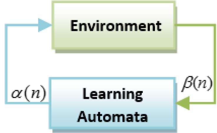
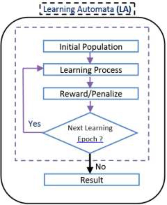
Learning Automata (LA) is perceived as an abstract model that selects an operation from a set of specific operations randomly. this algorithm employs the selected operation on the environment and informs the evaluated results by using a reinforcement signal (14). LA updates its interior states by means of selected operation and reinforcement signals. Then the algorithm selects the next operation in an iterative manner(15). The communication of LA and the environment is shown in Figure 1(16) .
The environment is shown by E={α,β,c} where α={α1 ,α2 ,...,αr} is a set of inputs, β={ β1 , β2 ,... βr} is a set of outputs, and c={ c1 , c2 ,... cr } is penalty probabilities. When β is a set of binary, so the environment is a P type. In this kind of environment β1=1 is considered as penalty and β2=0 as reward (17, 18).
Proposed Algorithms
In this paper two novel hybrid algorithms for QSAR feature selection problem are proposed. These two new hybrid algorithms take advantage of both genetic algorithm and learning automata. In below sections the application of genetic algorithm and learning automata are described for feature selection in QSAR problem and then, the MGALA and SGALA algorithms are explained.
Feature selection using GA
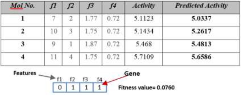
This algorithm tries to solve QSAR feature selection problem using Genetic Algorithm. The flowchart of this algorithm is depicted in Figure 2. At first this algorithm produces an initial population and then tries to converge to optimal result using genetic operations. Figure 3 shows a QSAR sample and corresponding chromosome for this algorithm.
The fitness function, crossover, and mutation operators are described in below sections:
Fitness function
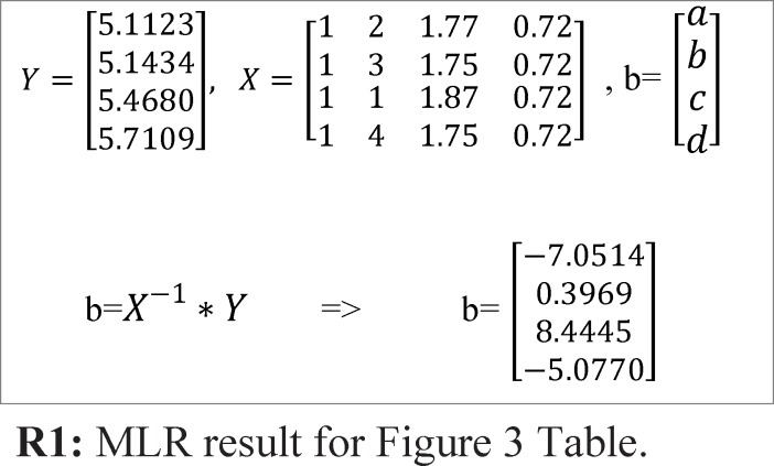
To obtain the fitness value, first by using Multiple Linear Regression (MLR), the activity is predicted and after that by using Root Mean Square Error (RMSE) equation, the fitness value of each chromosome/automaton is calculated. For example, for sample Table and chromosome of Figure 3, the fitness value is determined using below steps:
Step1: Predicting activity using MLR. By using MLR, the activity values can be predicted. R1 relation shows the application of MLR for the sample demonstrated in Figure 3.
For this specific example, the predicted activity values could be calculated using below function:
f=-7.0514+0.3969*f2+8.4445*f3 –5.0770*f4
Step 2: calculating chromosome fitness value using RMSE equation. After predicting activity values using MLR, the fitness value must be calculated using RMSE equation. R2 relation below shows the RMSE equation. In this function n is the number of sample molecules.
R2: fitness value using RMS function
Crossover operator
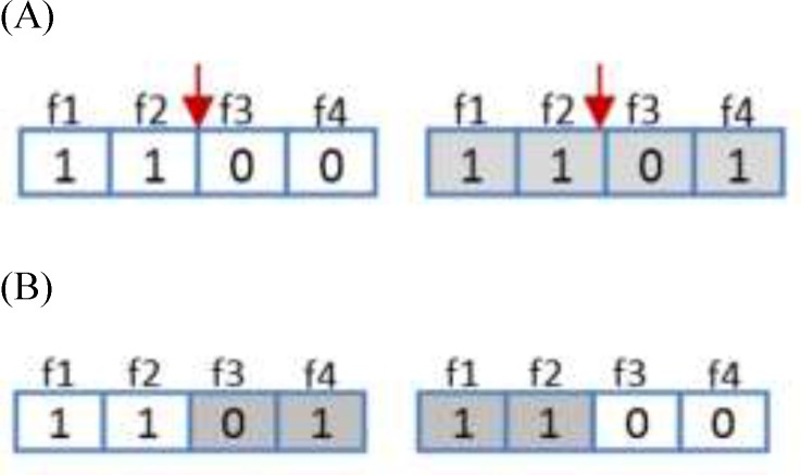
Regarding genetic algorithm, crossover operator applied to modify the contents of chromosomes from one generation to the next ones. It is similar to the biological crossover process that the GA is based. The crossover procedure takes more than one parent solutions and generating the same number of child solutions from them. The crossover operator in this algorithm uses single point crossover. In this type of crossover two random chromosomes were selected and half of each chromosome was attached to the other chromosome and vice versa. This operator is depicted in Figure 4.
Mutation operator
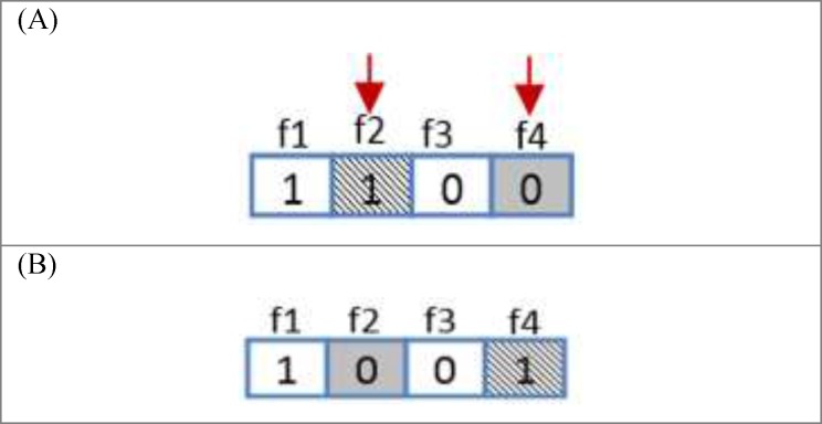
Similar to biological mutations, mutation operator is applied to sustain genetic variety from one generation of population to the next one. In mutation, the solution may alter completely from the previous solution. Therefore, GA can be improved to a better solution by using mutation. Mutation takes place in the course of evolution according to a user-defined mutation probability. The mutation operator type in this algorithm is order-based mutation. In this type of mutation two random genes are selected and the positions of them are swapped .This operator is illustrated in Figure 5.
GA Termination
In Genetic Algorithm there are some different conditions for termination of algorithm. In this paper at first the generation number is declared and then the algorithm executes according to this number.
Feature selection using LA
For a QSAR feature selection with n features, different 2n states exist and if LA is applied to solving QSAR feature selection problem, LA must involve 2n actions. In this article, the Object Migration Automata (OMA) method, proposed by Oommen and Ma, is utilized to reduce convergence speed. More precisely, the proposed algorithm utilizes Tsetlin automata, an OMA based algorithm, for solving QSAR selection problem (19).
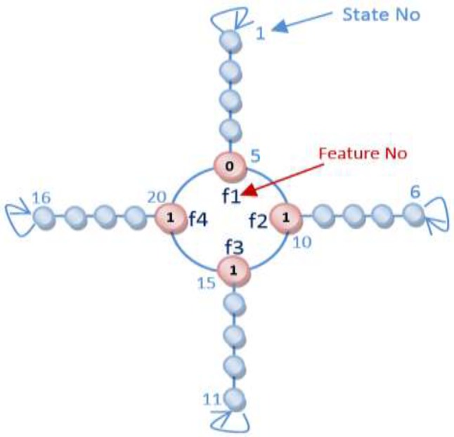
In our proposed algorithms each chromosome is equal to an automaton and each gene is equivalent to an action of an automaton. The automaton illustrated in Figure 6 is equal to the chromosome which was brought in Figure 3. The flowchart of Learning Automata for solving this problem is depicted in Figure 7. In this algorithm at first the initial population consisting of some random automata is generated, and then by using LA method it tries to converge to the optimal result. By repeating the process of learning, the LA selects the suitable position of actions.
Reward and penalize Operator
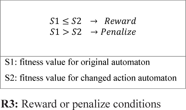
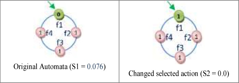
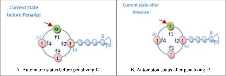
One of the important subjects in learning automata is reward and penalize operator. In this method in every epoch for every automaton an action is randomly selected and it is rewarded or penalized. At first the fitness value of automaton is calculated (suppose it is S1), after that if the selected action value is zero it changes to one and vice versa and then the fitness value of the altered automaton is calculated once again (suppose it is S2). Reward operator occurs when the value of S1 is equal to or smaller than the value of S2 and penalize operator occurs when the S1 value is bigger than S2 value (Figure 8). R3 relation shows the reward and penalizes.
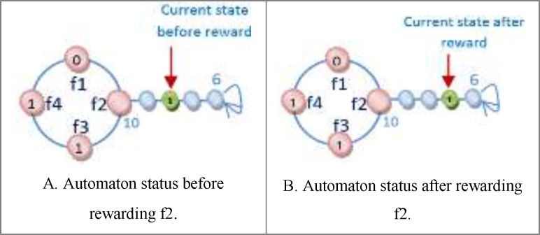
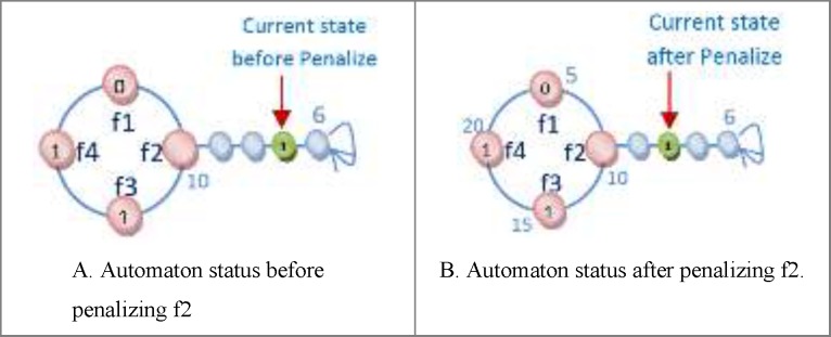
For Figure 8 automaton, the selected action is penalized, because by changing the selected action value from zero to one its fitness value is minimized (the error is minimized). If the fitness value for the changed action is larger than original automaton fitness value, therefore the automaton is penalized. Figure 9 shows the reward operation and figures 10 and 11 show penalize operation.
Two possibilities are likely when penalizing an action:
(a) The action might occur in a position other than frontier position. In this case, penalizing makes it less important. The way the action of feature f2 is penalized, is shown in Figure 10.
(b) The action could occur in frontier position. In this case, provided that the value of action is zero it is turned into one and Vice versa. Figure 11 shows how feature f1 is penalized.
Learning termination
For termination of learning process there are different methods such as: predefined epoch number and obtained suitable result and etc. In this paper we use predefined epoch number and at first before the start of algorithm, the epoch number is defined and the algorithm repeats learning process using epoch number value.
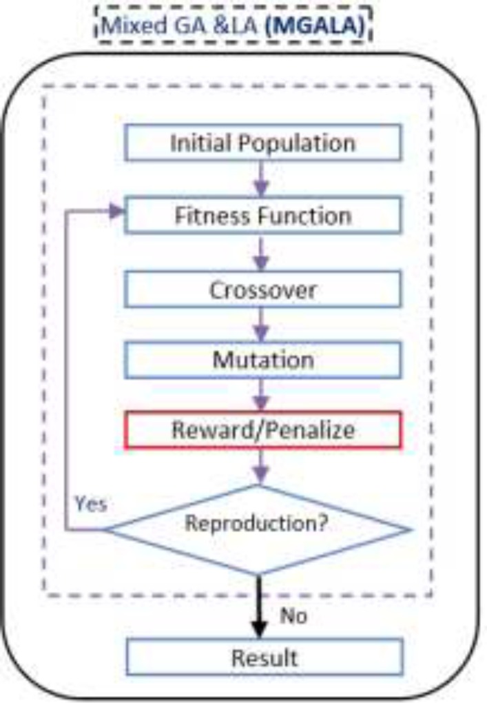
Mixed GALA Algorithm (MGALA)
GA tries to find the best chromosome in the population. In GA the location of genes, in chromosomes are random.
The optimal solution can be found in fewer generations if the position of the genes in the chromosomes discover optimally. Consequently, our algorithm tries to obtain the optimal solution in fewer generations utilizing the advantages of both GA and LA. In this algorithm the LA operator (reward/penalize) is added to GA. Generation number in GA and epoch number in LA in this algorithm are equivalent. The flowchart of this algorithm is shown in Figure 12.
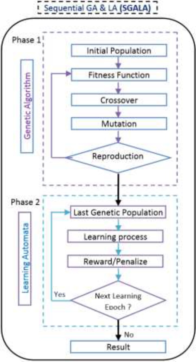
Sequential GALA Algorithm (SGALA)
Another algorithm that we have proposed in this paper is SGALA. In this Algorithm at first the GA tries to converge to optimal result after a number of GA generations, the last population of GA is applied as the initial population of LA and next the LA tries to improve the last GA results. In this algorithm we could optimize the initial population of GA using less generation numbers and then by using LA the result could be improved. Generation number in GA and Epoch number in LA are distinct. The flowchart of this algorithm is exhibited in Figure 13.
Results
In this section we examine and evaluate the proposed algorithms with three different datasets. At first, the Laufer et al. (8) dataset was used for evaluation and examination of our proposed algorithms against GA, LA, PSO, and ACO algorithms and after that the best results of all algorithms were used as input for LS-SVR classifier model in which the differences of the results were reported. Secondly, two other datasets by Guha et al.(9) and Calm et al. (10) were used for the evaluation of proposed algorithms against GA, LA, PSO, and ACO algorithms. In this part only the rate of convergence to optimal result of the proposed algorithms and all other algorithms were compared and also the results of feature selection using the proposed algorithms and other algorithms were compared to each other.
First experiment
Dataset
The dataset used in the first experiment is derived from the Laufer et al. study (8). Table 1 shows the general chemical structures and the structural details of these compounds. This set contains the inhibitory activity values of N-(3-(3-sulfamoylphenyl)-1H-indazol-5-yl)-acetamides and carboxamides against TTK, reported in IC50 (µM). The IC50 values were converted into pIC50 (-log IC50) values. pIC50 is the relevant variable that distinguishes the biological parameters for the developed QSAR model.
The inhibitory activities fall in the range 4.74 for inhibitors 6a and 14b to 8.54 for inhibitor 55d, with a mean value of 6.68. Table 1 depicts the basic structures of these inhibitors. The dataset was separated into two groups (training and test sets) using Y ranking method. The training and test sets consist of 44 and 11 inhibitors, respectively. The structures of molecules were drawn and optimized using HyperChem package (version 7.0) (20). The Semi-empirical AM1 algorithm with Polak–Ribiere was used as the optimization method until the root mean square gradient receives to 0.01 kcal mol-1 . The optimized geometries were used for the descriptor generation.
The Dragon software is used to calculate the molecular descriptors (21). The MATLAB software version 7.6 and the free LS-SVM toolbox version 1.5 was used to derive all the LS-SVM models (22).
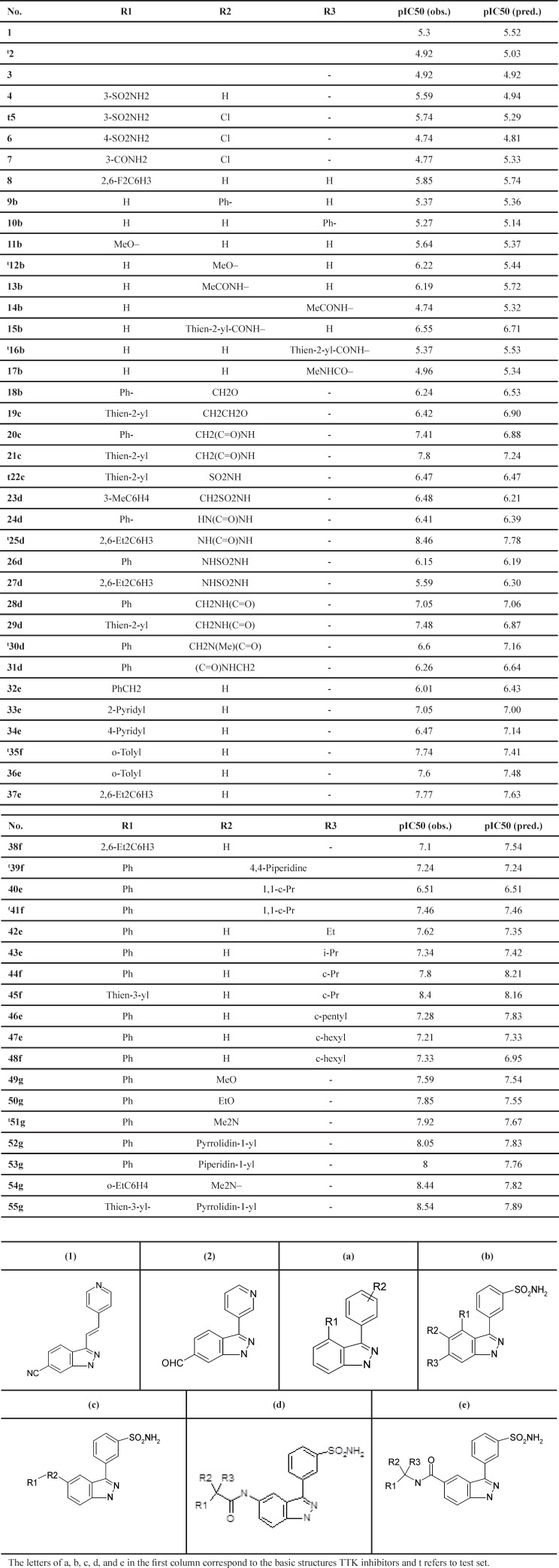
Compounds list, observed, predicted pIC50 values, and Basic structures of TTK inhibitors.
Parameters of Algorithms
| Algorithm | GA | ACO(3, 38) | PSO(4, 39) | LA | SGALA | MGALA |
|---|---|---|---|---|---|---|
| Initial Population | 100 | 100 | 100 | 100 | 100 | 100 |
| Generation | 100 | - | - | - | 60 | 100 |
| Epoch | - | 100 | 100 | 100 | 40 | - |
| Cross over | 0.7 | - | - | - | 0.7 | 0.7 |
| Mutation | 0.3 | - | - | - | 0.3 | 0.3 |
| Memory | - | - | - | 3 | 3 | 3 |
| Inertia weight(w) | - | - | 0.8 | - | - | - |
| Acceleration constants | - | - | 1.5 | - | - | - |
| Rho | - | 0.7 | - | - | - | - |
Results of algorithms for ten different Runs (Laufer et al. dataset
| Algorithm | RMSE train | Running time (second) | |
|---|---|---|---|
| GA | |||
| Avg. | 0.8351 | 0.44203 | 70.1 |
| min | 0.8274 | 0.4369 | 65 |
| Max | 0.839 | 0.4523 | 76 |
| (Std.) | 0.0035 | 0.0048 | 2.982 |
| Best Result (feature names) | D/Dr05, MATS5m, MATS3v, ATS6e, SPAM, RDF035m, Mor08m, nCt | ||
| ACO | |||
| Avg. | 0.825 | 0.454 | 93.144 |
| min | 0.800 | 0.435 | 79.65 |
| Max | 0.840 | 0.486 | 106.5 |
| (Std.) | 0.010 | 0.014 | 8.736 |
| Best Result (feature names) | AMW, nCIR, RBN, DECC, BELp1, Mor17u, E3u, R1p+ | ||
| PSO | |||
| Avg. | 0.81796 | 0.46421 | 4.75012 |
| min | 0.8001 | 0.4255 | 4.2001 |
| Max | 0.8473 | 0.4868 | 5.721 |
| (Std.) | 0.0137 | 0.0178 | 0.4568 |
| Best Result (feature names) | RDF095m, C-008, RBN, ISH, SPAM, GATS6e, MATS6e, nCaH | ||
| LA | |||
| Avg. | 0.8263 | 0.4535 | 134.3 |
| min | 0.814 | 0.438 | 118 |
| Max | 0.8382 | 0.4695 | 170 |
| (Std.) | 0.0071 | 0.0092 | 19.4784 |
| Best Result (feature names) | BEHv1,MATS3m,SPAM,RDF095m, Mor03u , Mor03m, E1u, nCaH | ||
| SGALA | |||
| Avg. | 0.8470 | 0.4256 | 80.4 |
| min | 0.8315 | 0.4074 | 72 |
| Max | 0.86 | 0.4469 | 89 |
| (Std.) | 0.0071 | 0.0099 | 5.5892 |
| Best Result (feature names) | RBN, X1A, BIC4, GATS5v, RDF035m, E2m, HATS1u, H8m | ||
| MGALA | |||
| Avg. | 0.8647 | 0.4003 | 118.4 |
| min | 0.8596 | 0.3868 | 111 |
| Max | 0.8737 | 0.4079 | 125 |
| (Std.) | 0.0040 | 0.0060 | 4.4581 |
| Best Result (feature names) | RBN, PW3, SAM, RDF095m, RDF120m, nSO2, C-027,H-046 | ||
The statistical parameters of the GA-LS-SVR, ACO-LS-SVR, PSO-LS-SVR, LA-LS-SVR, SGALA-LS-SVR, and MGALA- LS-SVR models
| Parameters | γ | δ2 | R2 train | RMSE train | R2 test | RMSE test |
|---|---|---|---|---|---|---|
| GA- LS-SVR | 468.323 | 1413.690 | 0.861 | 0.409 | 0.760 | 0.591 |
| ACO- LS-SVR | 74.4881 | 88.5071 | 0.9028 | 0.3440 | 0.8980 | 0.4842 |
| PSO- LS-SVR | 8.2448 | 23.6189 | 0.9290 | 0.2965 | 0.8147 | 0.5578 |
| LA-LS-SVR | 27.965 | 19.1907 | 0.964 | 0.210 | 0.786 | 0.545 |
| SGALA-LS-SVR | 119.877 | 465.674 | 0.880 | 0.381 | 0.875 | 0.443 |
| MGALA-LS-SVR | 1007.3 | 293.604 | 0.940 | 0.268 | 0.770 | 0.564 |
The statistical parameters of the external test set for GA-LS-SVR, ACO-LS-SVR, PSO-LS-SVR, LA-LS-SVR, SGALA-LS-SVR, and MGALA-LS-SVR models
| Parameters | GA- LS-SVR | ACO- LS-SVR | PSO- LS-SVR | LA- LS-SVR | SGALA-LS-SVR | MGALA-LS-SVR |
|---|---|---|---|---|---|---|
| 0.698 | 0.803 | 0.731 | 0.744 | 0.830 | 0.725 | |
| 0.759 | 0.898 | 0.815 | 0.786 | 0.875 | 0.770 | |
| 0.665 | 0.897 | 0.772 | 0.776 | 0.859 | 0.750 | |
| 0.758 | 0.880 | 0.815 | 0.769 | 0.875 | 0.759 | |
| 0.123 | 0.001 | 0.053 | 0.012 | 0.018 | 0.026 | |
| 0.001 | 0.020 | 0.000 | 0.0201 | 0.000 | 0.014 | |
| 0.526 | 0.870 | 0.646 | 0.709 | 0.764 | 0.661 | |
| 0.734 | 0.777 | 0.815 | 0.685 | 0.875 | 0.689 | |
| 0.954 | 0.952 | 0.950 | 0.969 | 0.963 | 0.964 | |
| 1.041 | 1.047 | 1.048 | 1.026 | 1.035 | 1.031 |
Results of algorithms for ten different Runs (Guha et al. and Calm et al. datasets
| Dataset 1 | Dataset 2 | |||||||||||||
|---|---|---|---|---|---|---|---|---|---|---|---|---|---|---|
| Feature size | Mol no. | References | Selected features no. | Feature size | Mol no. | References | Selected features no. | |||||||
| 320 | 79 | (9) | 12 | 115 | 45 | (10) | 7 | |||||||
| RMSE train | Running time (second) | RMSE train | Running time (second) | |||||||||||
| GA | ||||||||||||||
| Avg. | 0.626 | 0.413 | 220.184 | 0.953 | 0.348 | 40.332 | ||||||||
| min | 0.616 | 0.401 | 189.797 | 0.946 | 0.283 | 36.935 | ||||||||
| Max | 0.647 | 0.419 | 291.226 | 0.969 | 0.376 | 48.873 | ||||||||
| (Std.) | 0.009 | 0.005 | 27.303 | 0.006 | 0.027 | 3.740 | ||||||||
| Best Result (feature names) | MOLC#5, EMAX#1, MOMI#3, GRAV#3, CHDH#2, CHDH#3, SCDH#1, SAAA#1, SAAA#3, CHAA#2, ACHG#0 | BEHm2, ATS1m, MATS1m, DISPe, RDF020u, E3s, HTp | ||||||||||||
| ACO | ||||||||||||||
| Avg. | 0.596 | 0.428 | 101.835 | 0.934 | 0.413 | 15.344 | ||||||||
| min | 0.564 | 0.415 | 86.5 | 0.923 | 0.379 | 12.196 | ||||||||
| Max | 0.613 | 0.446 | 116.54 | 0.945 | 0.448 | 26.201 | ||||||||
| (Std.) | 0.016 | 0.009 | 10.237 | 0.007 | 0.022 | 4.081 | ||||||||
| Best Result (feature names) | MOLC#4, WTPT#2, WTPT#5, MDEC#12, MDEN#33, MREF#1, GRVH#3, NITR#5, FNSA#2, SADH#3, CHDH#3, FLEX#5 | AMW, Me, X4v, IDDE, L3m, HTp, nROR | ||||||||||||
| PSO | ||||||||||||||
| Avg. | 0.603 | 0.425 | 7.057 | 0.931 | 0.422 | 5.728 | ||||||||
| min | 0.583 | 0.410 | 0.627 | 0.9164 | 0.3821 | 4.233 | ||||||||
| Max | 0.632 | 0.436 | 11.147 | 0.9445 | 0.4687 | 7.781 | ||||||||
| (Std.) | 0.018 | 0.010 | 2.662 | 0.008 | 0.027 | 1.127 | ||||||||
| Best Result (feature names) | 2SP2#1, CHAA#2, CHDH#2, WNSA#1, WTPT#4, PNSA#2, N2P#1, SADH#2, SADH#1, NITR#5, SURR#1, MOLC#3 | R1u, nF, S2K, nROR, L3m, AMW, HTp | ||||||||||||
| LA | ||||||||||||||
| Avg. | 0.61146 | 0.4215 | 265.617 | 0.940 | 0.393 | 56.644 | ||||||||
| min | 0.5945 | 0.4022 | 215.16 | 0.934 | 0.372 | 44.469 | ||||||||
| Max | 0.646 | 0.430 | 307.315 | 0.947 | 0.413 | 74.579 | ||||||||
| (Std.) | 0.016 | 0.008 | 31.762 | 0.003 | 0.012 | 9.514 | ||||||||
| Best Result (feature names) | V3CH#15, WTPT#4, MDEC#34, MDEO#12, MREF#1, EMIN#1, MOMI#1, VOL#150, homo#0, WPSA#1, FNHS#1, RNH#1 | ATS2e, RPCG, DISPe, L3m, H0e, HTp, F082 | ||||||||||||
| SGALA | ||||||||||||||
| Avg. | 0.6409 | 0.4051 | 270.678 | 0.955 | 0.340 | 61.969 | ||||||||
| min | 0.624 | 0.382 | 245.521 | 0.946 | 0.312 | 46.548 | ||||||||
| Max | 0.680 | 0.414 | 298.413 | 0.962 | 0.374 | 76.731 | ||||||||
| (Std.) | 0.017 | 0.009 | 18.779 | 0.005 | 0.019 | 9.553 | ||||||||
| Best Result (feature names) | KAPA#2, KAPA#4, ALLP#1, ALLP#2, V4PC#12, N6CH#16, N7CH#20, NITR#5, FNSA#3, RNCG#1, SCDH#2, FNHS#1 | IDDE, SHP2, DISPe, L3m, H0e, HTp, Hy | ||||||||||||
| MGALA | ||||||||||||||
| Avg. | 0.704 | 0.371 | 627.026 | 0.960 | 0.322 | 124.922 | ||||||||
| min | 0.684 | 0.352 | 555.923 | 0.958 | 0.302 | 89.526 | ||||||||
| Max | 0.727 | 0.390 | 709.474 | 0.965 | 0.329 | 150.749 | ||||||||
| (Std.) | 0.013 | 0.010 | 53.150 | 0.001 | 0.007 | 20.326 | ||||||||
| Best Result (feature names) | KAPA#2, KAPA#4, ALLP#4, V5CH#17, S6CH#18, MOLC#1, SADH#2, CHDH#1, CHDH#3, SAAA#2, ACHG#0, SURR#5 | GGI1, DISPe, RDF020u, E3s, H0e, HTp, Hy | ||||||||||||
Descriptor calculation and selection
These descriptors were presented in a two dimensional data matrix whose rows and columns store the inhibitors and descriptors, respectively. Some preprocessing operations should be applied after calculating the molecular descriptors. Then the following procedure selects some of the important descriptors. At the beginning, those descriptors that remained constant for all the inhibitors were ignored. Variable pairs with a Pearson correlation coefficient larger than 0.80 were considered as inter-correlated. One of them was used to develop the feature selection model and the other one was ignored. After this process, totally 221 descriptors remained for further investigation.
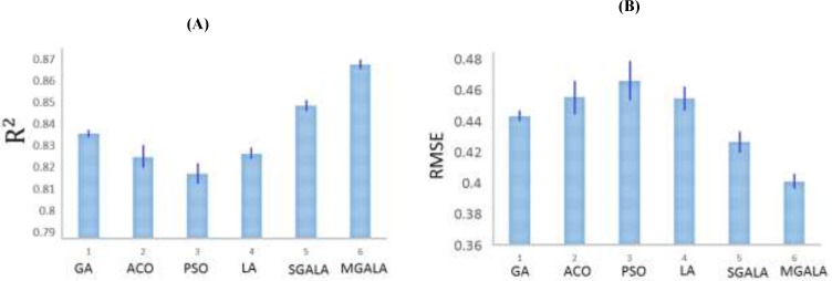
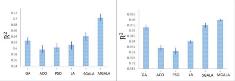
Subsequently, the GA, ACO, PSO, LA, SGALA, and MGALA algorithms were used to select the most feasible descriptors from 221 remained descriptors which were related to the anti-cancer activity of inhibitors. In this paper for performance evaluating of algorithms we used MATLAB software environment. For all of the four algorithms we implemented code in MATLAB and then results of proposed algorithms in different runs were evaluated and compared with each other. All runs were performed on AMD Phenom II Quad-core 1.8 GHz and 4 Gb Ram. Our examinations are done on anti-Cancer datasets. This dataset has 55 molecule and 221 descriptors. So our proposed algorithms tries to find some features that minimize Error value or maximize R2 value. It is suggested that the number of samples should be 5 times larger than the number of features (23, 24). Therefore, maximum number of feature that our proposed algorithms try to find it is 20% of inhibitor numbers in the training set. The results of all the algorithms are explained in Tables 3. The mean R2 of SGALA and MGALA is higher than those of other algorithms and the mean RMSE value of our proposed algorithms is less than those of others. The properties of algorithms are demonstrated in Table 2. The variations of RMSE and R2 values for this Table are depicted in Figure 14.
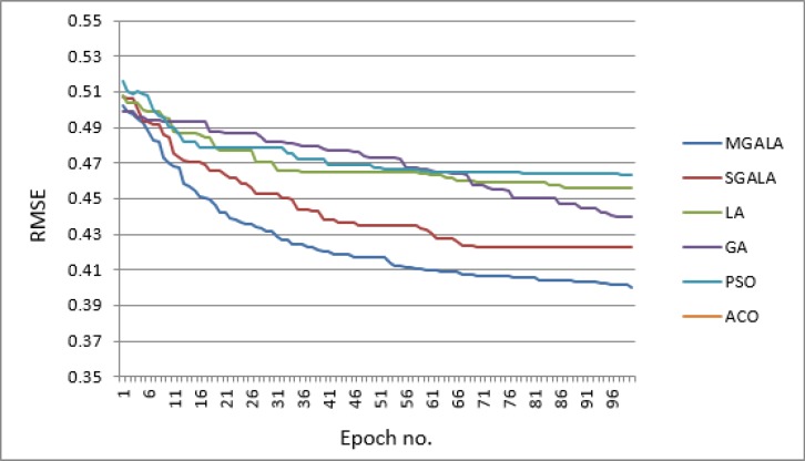
In Figure 15, the process of convergence to optimal result for proposed algorithms and other algorithms is depicted. In this figure every result is the average of ten random executions. Itʹs evident that the MGALA and SGALA convergence rates are better than those of others and the convergence rate of MGALA algorithm is even better than SGALA algorithm. The final results of MGALA and SGALA are better than other algorithms.
LS-SVR Model
For the modeling studies we selected best runs from algorithms which present a good combination of R2 and RMSE results. To investigate relation between selected molecular descriptors and pIC50, we used Least Squares-Support Vector Regression (LS-SVR) as a non-linear feature mapping technique. In this model, the input vectors are the set of descriptors selected by feature selection algorithms.
The radial basis function (RBF) was utilized as a kernel function, which represents the distribution of sample in the mapping space. RBF is a non-linear function and can reduce the computational complexity of training procedure (25). The next step was optimization of LS-SVR parameters, including regularization parameter (γ) and kernel parameter (δ2).
The optimized values for the parameters were achieved from grid search method. As mentioned before it, all algorithms introduced in this paper have used LS_SVR model and RBF kernel function. Sigma value of RBF kernel function is effective in model generation. The Higher is sigma value, the more flat is Gaussian distribution; so the decision boundary is smoother. Lower sigma value of RBF kernel function will make sharper the Gaussian distribution and also the decision boundary will be more flexible (26). The best value of sigma which enhances the model performance is achieved using grid search method. The sigma values of all mentioned models are inserted in Table 4. The sigma values of SGALA-LS-SVR and MGALA-Ls-SVR models are proper than other models so their Gaussian distribution is not sharp or smooth.
Besides sigma parameter which has influence on model regression, the gamma regulation value minimizes training error and model complexity. Over-fitting will occur if values of sigma and gamma are enhanced (27, 28). Therefore, these values must be carefully selected. We observe that the sigma and gamma values of SGALA-LS-SVR and MGALA-Ls-SVR models are not maximum value simultaneously in Table.4. The parameter values inserted in Table.5 show that proposed models are acceptable.
The significance and predictability of the constructed model was evaluated using the external set and the statistical parameters were recommended by Trospsha (29, 30) and Roy (31). They suggested a number of criteria that assess the predictive ability of a QSAR model;
R4:
R5:
R6:
R7: 0.85 ≤ k ≤ 1.15 or 0.85 ≤
R8:
The statistical parameters of the GA- LS-SVR, ACO-LS-SVR, PSO-LS-SVR, LA-LS-SVR, SGALA-LS-SVR, and MGALA-LS-SVR models were compared. The results are given in Table 5. All models have Q2 values larger than 0.5 and rp2 values higher than 0.6.
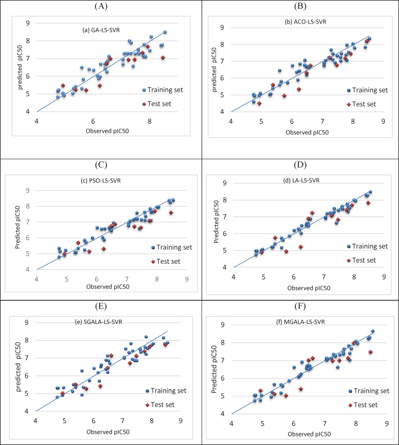
The performance of all models was evaluated by plotting the predicted values of pIC50 against experimental values for the training and test sets. The results are shown in Figure 16.
This figure shows that there is a good agreement between the observed activity and the predicted values.
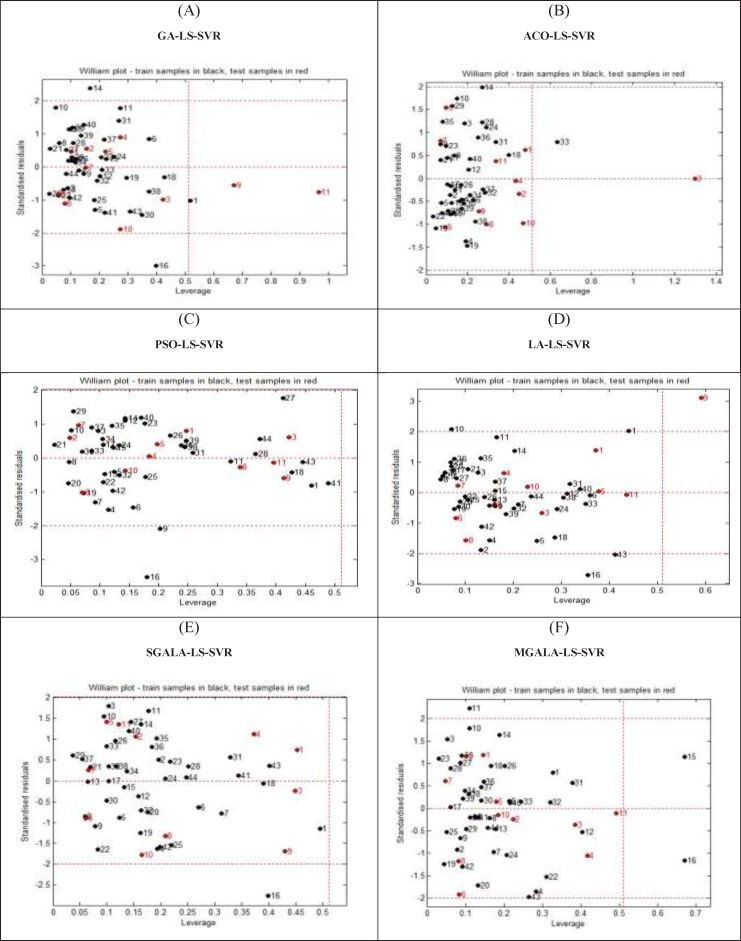
Applicability Domain assessment
One of the crucial problems in QSAR modeling is the definition of its Applicability Domain (AD). There are different methods for obtaining applicability domain in QSAR models (32). One of the common methods is defining leverage values for every compound (33). In this work, the applicability domain is verified by the William’s plot. The applicability domain is settled inside a squared range within ±3 standard deviation and a leverage threshold
Cross-Validation
To assure the impartial comparison of the classification outputs and in order to avoid generating random results, this study applied a Leave-One-Out cross validation (LOOCV) methodology. Cross-validation is a statistical procedure that divides data into two segments for comparing and evaluating learning algorithms. One part is usually used to learn or train the model and the other is applied to validate the model (36)
Second experiment
In this section all of the mentioned algorithms are applied on Guha et al.(9) and Calm et al. (10) datasets. For all of the datasets, 80% of data were assumed as train data and next 20% data were assumed as test data. The LOOCV cross-validation method was used for classification results. Because the number of features that algorithms try to find is 20% of inhibitor numbers in the training set, therefore for Guha et al. dataset the number of selected features was 12 and for Calm et al. dataset were 7. The properties of algorithms are demonstrated in Table 6. The variations of R2 values for this Table are depicted in Figure 18.
In Figure 19 the process of converging to optimal result for proposed algorithms and other mentioned algorithms are depicted. In this figure every result is the average of ten random executions. Itʹs evident that the MGALA and SGALA converging rates are better than those of others and the converging rate of MGALA algorithm is even better than SGALA algorithm for Guha et al. and Calm et al. datasets. The final results of MGALA and SGALA are better than all other algorithms.
Discussion
Descriptor selection has been used with various algorithms on QSAR data. Using the same data is essential in order to compare algorithms. As mentioned in the manuscript, SGALA and MGALA algorithms are suggested for descriptor selection. We implemented PSO, GA, and ACO algorithms because these algorithms had been applied on different data not available now. The results of proposed algorithms have been compared with GA, PSO, and ACO algorithms. The acquired results are descripted as follow:
In reference (4), Goodarzi et al have proposed two GA and PSO algorithms using three different regression methods as: multiple linear Regression (MLR), Locally Weighted Regression based on Euclidean distance (LWRE), and Locally Weighted Regression based on Mahalanobis distance (LWRM).
All of the algorithms had been implemented on “imidazo[1,5-a]pyrido[3,2-e]pyrazines, inhibitors of phosphodiesterase 10A” dataset with 46 train and 15 test compounds. In this paper reported R2train values on PSO/MLR, GA/MLR, PSO/LWRE, PSO/LWRM, GA/LWRE, and GA/LWRM were 0.82, 0.85, 0.81, 0.81, 0.85, and 0.85 respectively. Also R2test reported values were 0.87, 0.79, 0.89, 0.87, 0.76, and 0.76 respectively. In another work (37), GA/MLR had been executed on “imidazo[1,5-a]pyrazine derived ACK1 inhibitors” dataset and the reported value for R2train over 30 samples was 0.8. Ant colony optimization algorithm along with PLS, MLR, and SVM regressions had been executed on “anti-HIV-1 activities of 3-(3,5-dimethylbenzyl)uracil derivatives” datasets (3). In this research, produced R2train values for ACO/MLR, ACO/SVM, and ACO/PLS on 34 compounds were 0.983, 0.991, and 0.983 respectively and R2test values on 9 compounds were 0.942, 0.991, and 0.945 respectively.
In our work GA/MLR, ACO/MLR, PSO/MLR, LA/MLR, SGALA/MLR, and MGALA/MLR have been executed on three different datasets. Our proposed SGALA/MLR and MGALA/MLR algorithms have produced better results than those of GA/MLR, ACO/MLR, and PSO/MLR algorithms . Therefore, it is expected that the results will be better by executing our proposed new algorithms on different QSAR datasets.
Conclusion
In this paper two novel hybrid algorithms based on Learning Automata and Genetic Algorithm have been proposed for feature selection in QSAR. Through implementing and running all the algorithms with different datasets, it was observed that the rate of converging to optimal results in MGALA and SGALA algorithms are better than GA, ACO, PSO, LA algorithms and the rate of MGALA algorithm is better than SGALA and all other algorithms. A very important difference between LA and GA is that the GA tries to find the most appropriate chromosome from the population, but in LA the position of action is very important and therefore by combining these two algorithms (MGALA) the rate of converging is improved. Error value in MGALA and SGALA algorithms is smaller than GA, ACO, PSO, and LA algorithms and R2 value in SGALA and MGALA algorithms is more than GA, ACO, PSO, and LA algorithms in most runs as well. Different runs for all algorithms demonstrated that the produced results by MGALA algorithms are better than SGALA algorithm and SGALA algorithm is better than all GA, ACO, PSO, and LA algorithms. After selecting some features using GA, ACO, PSO, LA, SGALA, and MGALA algorithms, the output of algorithms was applied separately as the input of LS-SVR model. The results of GA-LS-SVR, ACO-LS-SVR, PSO-LS-SVR, LA-LS-SVR, SGALA-LS-SVR, and MGALA-LS-SVR models have proved that the SGALA-LS-SVR and MGALA-LS-SVR models are of high predictive ability and are able to fulfill all the criteria. These results have revealed that the performances of the SGALA-LS-SVR and MGALA-LS-SVR models are superior to those of GA- LS-SVR, ACO-LS-SVR, PSO-LS-SVR, and LA-LS-SVR models.
References
-
1.
Chin A, Mirzal A, Haron H, Hamed H. Supervised, Unsupervised and Semi-supervised Feature selection: A Review on Gene Selection. 2015.
-
2.
Goodarzi M, Dejaegher B, Heyden YV. Feature selection methods in QSAR studies. Journal of AOAC International. 2012;95:636-51. [PubMed ID: 22816254].
-
3.
Goodarzi M, Freitas MP, Jensen R. Ant colony optimization as a feature selection method in the QSAR modeling of anti-HIV-1 activities of 3-(3, 5-dimethylbenzyl) uracil derivatives using MLR, PLS and SVM regressions. Chemometrics and intelligent laboratory systems. 2009;98:123-9.
-
4.
Goodarzi M, Saeys W, Deeb O, Pieters S, Vander Heyden Y. Particle swarm optimization and genetic algorithm as feature selection techniques for the QSAR modeling of imidazo [1, 5-a] pyrido [3, 2-e] pyrazines, inhibitors of phosphodiesterase 10A. Chemical biology & drug design. 2013;82:685-96. [PubMed ID: 23906083].
-
5.
Shen Q, Jiang J-H, Tao J-c, Shen G-l, Yu R-Q. Modified ant colony optimization algorithm for variable selection in QSAR modeling: QSAR studies of cyclooxygenase inhibitors. Journal of chemical information and modeling. 2005;45:1024-9. [PubMed ID: 16045297].
-
6.
Nantasenamat C, Monnor T, Worachartcheewan A, Mandi P, Isarankura-Na-Ayudhya C, Prachayasittikul V. Predictive QSAR modeling of aldose reductase inhibitors using Monte Carlo feature selection. European journal of medicinal chemistry. 2014;76:352-9. [PubMed ID: 24589490].
-
7.
Zhou X, Li Z, Dai Z, Zou X. QSAR modeling of peptide biological activity by coupling support vector machine with particle swarm optimization algorithm and genetic algorithm. Journal of Molecular Graphics and Modelling. 2010;29:188-96. [PubMed ID: 20621530].
-
8.
Laufer R, Ng G, Liu Y, Patel NKB, Edwards LG, Lang Y, Li S-W, Feher M, Awrey DE, Leung G. Discovery of inhibitors of the mitotic kinase TTK based on N-(3-(3-sulfamoylphenyl)-1H-indazol-5-yl)-acetamides and carboxamides. Bioorganic & medicinal chemistry. 2014;22:4968-97. [PubMed ID: 25043312].
-
9.
Guha R, Jurs PC. Development of linear, ensemble, and nonlinear models for the prediction and interpretation of the biological activity of a set of PDGFR inhibitors. Journal of chemical information and computer sciences. 2004;44:2179-89. [PubMed ID: 15554688].
-
10.
Calm JM, Hourahan G. Refrigerant data update. HPAC Engineering. 2007;79:50-64.
-
11.
Melanie M. An introduction to genetic algorithms. 3. Fifth printing. Cambridge, Massachusetts London, England; 1999.
-
12.
Masoudi-Sobhanzadeh Y, Motieghader H. World Competitive Contests (WCC) algorithm: A novel intelligent optimization algorithm for biological and non-biological problems. Informatics in Medicine Unlocked. 2016;3:15-28.
-
13.
Wu AS, Yu H, Jin S, Lin K-C, Schiavone G. An incremental genetic algorithm approach to multiprocessor scheduling. Parallel and Distributed Systems, IEEE Transactions on. 2004;15:824-34.
-
14.
Narendra KS, Thathachar MA. Learning automata: an introduction. Courier Corporation; 2012.
-
15.
Thathachar M, Narendra K. Learning Automata, an Introduction. NJ: Prentice Hall International, Englewood Cliffs; 1989.
-
16.
Ghader HM, KeyKhosravi D, HosseinAliPour A. DAG scheduling on heterogeneous distributed systems using learning automata, in Intelligent Information and Database Systems. Springer; 2010. p. 247-57.
-
17.
Meybodi M, Beigy H. New Class of Learning Automata Based Schemes for Adaptation of Bachpropagation Algorithm Parameters. Iranian Journal of Science and technology (to appear). 1998.
-
18.
Oommen BJ, Ma DCY. Deterministic learning automata solutions to the equipartitioning problem. IEEE Transactions on Computers. 1988:2-13.
-
19.
Horn G, Oommen BJ. A fixed-structure learning automaton solution to the stochastic static mapping problem. in Parallel and Distributed Processing Symposium, 2005. Proceedings. 19th IEEE International. IEEE; 2005.
-
20.
-
21.
Todeschini R, Consonni V, Mauri A, Pavan M. DRAGON-Software for the calculation of molecular descriptors. Web version. 2003;3.
-
22.
Suykens JA, Van Gestel T, De Moor B, Vandewalle J. Basic Methods of Least Squares Support Vector Machines, in Least Squares Support Vector Machines. World Scientific; 2002.
-
23.
Hatcher L. A step-by-step approach to using the SAS system for factor analysis and structural equation modeling Cary, North Carolina. SAS Institute; 1994, Inc.
-
24.
Bryant FB, Yarnold PR. Principal-components analysis and exploratory and confirmatory factor analysis. 1995.
-
25.
Ensafi AA, Hasanpour F, Khayamian T. Simultaneous chemiluminescence determination of promazine and fluphenazine using support vector regression. Talanta. 2009;79:534-8. [PubMed ID: 19559917].
-
26.
Han L, Embrechts M, Szymanski B, Sternickel K, Ross A. Sigma tuning of gaussian kernels: detection of ischemia from magnetocardiograms. Google Patents; 2013.
-
27.
Chandaka S, Chatterjee A, Munshi S. Cross-correlation aided support vector machine classifier for classification of EEG signals. Expert Systems with Applications. 2009;36:1329-36.
-
28.
Suykens JA, Vandewalle J. Least squares support vector machine classifiers. Neural processing letters. 1999;9:293-300.
-
29.
Tropsha A, Gramatica P, Gombar VK. The importance of being earnest: validation is the absolute essential for successful application and interpretation of QSPR models. QSAR & Combinatorial Science. 2003;22:69-77.
-
30.
Alexander G, Alexander T. Beware of Q2. J Mol Graph Model. 2002;20:269-76. [PubMed ID: 11858635].
-
31.
Roy PP, Roy K. On some aspects of variable selection for partial least squares regression models. QSAR & Combinatorial Science. 2008;27:302-13.
-
32.
Eriksson L, Jaworska J, Worth AP, Cronin MT, McDowell RM, Gramatica P. Methods for reliability and uncertainty assessment and for applicability evaluations of classification-and regression-based QSARs. Environmental health perspectives. 2003;111:1361. [PubMed ID: 12896860].
-
33.
Gramatica P. Principles of QSAR models validation: internal and external. QSAR & combinatorial science. 2007;26:694-701.
-
34.
Sahigara F, Ballabio D, Todeschini R, Consonni V. Assessing the validity of QSARs for ready biodegradability of chemicals: an applicability domain perspective. Current computer-aided drug design. 2013;10:137-47.
-
35.
Sahigara F, Mansouri K, Ballabio D, Mauri A, Consonni V, Todeschini R. Comparison of different approaches to define the applicability domain of QSAR models. Molecules. 2012;17:4791-810. [PubMed ID: 22534664].
-
36.
Chen K-H, Wang K-J, Tsai M-L, Wang K-M, Adrian AM, Cheng W-C, Yang T-S, Teng N-C, Tan K-P, Chang K-S. Gene selection for cancer identification: a decision tree model empowered by particle swarm optimization algorithm. BMC bioinformatics. 2014;15:49. [PubMed ID: 24555567].
-
37.
Pourbasheer E, Aalizadeh R, Ganjali MR, Norouzi P, Shadmanesh J. QSAR study of ACK1 inhibitors by genetic algorithm–multiple linear regression (GA–MLR). Journal of Saudi Chemical Society. 2014;18:681-8.
-
38.
Dorigo M, Blum C. Ant colony optimization theory: A survey. Theoretical computer science. 2005;344:243-78.
-
39.
Eberhart RC, Shi Y. Particle swarm optimization: developments, applications and resources. in Evolutionary Computation, 2001. Proceedings of the 2001 Congress on. IEEE; 2001.