
Abstract
This paper describes a multi-species and multi-mechanism reactive-transport modelling framework for concrete. This modelling framework has the potential to be used in conjunction with performance specifications currently being developed in the US. The modelling framework is ‘nearly’ self-sufficient as it enables electrical resistivity to be used as the main physically measured input parameter in the simulations. The model uses thermodynamic calculations to predict pore solution composition, pore solution resistivity, pore volumes, and reactions between the solid and ionic components of the cementitious matrix such as chloride binding. The measured electrical resistivity is normalized by the calculated pore solution resistivity to compute the formation factor, which is used to predict transport properties of the ionic species. The framework allows the solution of reactive-transport equations with minimal input data to assess ionic movement, chloride ingress, and time to corrosion.
1 Introduction
1.1 Reflections on the 50th anniversary of Material and Structures
On the 50th anniversary of RILEM, Wittman [1] encouraged us to “pause from the hectic pace of our daily routine” and “take a closer look at the past.” This issue marks the 50th anniversary of the RILEM Materials and Structures (M&S) journal. This provides us with an opportunity to look back on what the authors in M&S have brought the profession. This also provides us an opportunity to look forward. The authors have been fortunate to have a strong connection with RILEM and are incredibly thankful for the formative role RILEM and its members have played in their professional and personal lives. Further, we recognize that RILEM is a distinctive and unique organization that provides a great service to the profession in three primary ways: (1) enabling international exchange of ideas, (2) providing high level scientific discussions on the material science of construction materials (this has long been a core of RILEM even before this was en vogue) [2], and (3) bridging the gap between science and practice. Nowhere is evidence of the primary benefits of RILEM more tangible than in the M&S Journal. On the 50th anniversary of the journal, we want to take this moment to say thank you and to wish M&S continued success over the next 50 years.
Due to the “anniversary nature of this issue” it is appropriate to note that in just the second year of M&S papers started to appear that discussed the durability of reinforced concrete structures exposed to salt contained in seawater [3]. By year three, M&S saw it summarizing the thoughts of legendary experts participating in Technical Committees (TC’s) on Concrete Durability (RILEM CDC) that describe the importance to fluid transport, freezing and saturation, and corrosion [4]. Additionally, the second to last article in the third year of the journal provided “News from USA”. As such, we will attempt to bring these topics together in an article that shares efforts the authors have been focused on in the US to bridge the gap between practice and science through performance specifications for concrete in conjunction with the American Association of State and Highway Transportation Officials (AASHTO-PP84-16) [5].
1.2 Toward performance specifications
The AASHTO PP-84 performance specification effort focuses on improving the durability of concrete pavements through the use of performance measures. While AASHTO-PP-84 contains many areas of interest, the five main areas in which the authors have been actively involved include: (1) Transport and the Formation Factor, (2) Freeze-Thaw Performance, (3) Deicing Salt Damage, (4) Porosity and Degree of Saturation, and (5) Restrained Shrinkage Cracking. Describing each of these sections is beyond the scope of this article and for information on those topics the reader is referred to other articles [6,7,8,9,10,11]. This paper discusses the topic of transport and the formation factor.
Figure 1 illustrates the general principles of using field tests to obtain fundamental material properties that can be used in mathematical models in conjunction with exposure conditions and construction geometries to estimate performance. The authors believe that with this estimated performance rational specifications can be developed that will relate performance with establish field acceptance measurement values. It can be argued that electrical resistivity testing can be transformed to the formation factor and the formation factor can then be used in transport models (for models that include sorption, diffusion or permeability) [6, 7, 12]. The vast majority of the work performed for AASHTO PP-84 to date has focused on the experimental measurement of physical properties. Rather than discussing AASHTO PP-84 test methods, this paper is part of an ongoing conversation as to whether computational tools can be used to supplement or supplant some of the physical testing in AASHTO PP-84. Research has shown the benefits of computational tools for the deicing salt damage [13, 14] and work has shown great promise for freeze-thaw models [15]. This paper will specifically discuss electrical resistivity, pore solution, formation factor, chloride binding and chloride ingress on its way to the prediction of reinforcing steel corrosion. This would enable AASHTO PP-84 to be extended in two exciting ways. First, it could be used in concrete structures containing reinforcing steel and not only pavements. Second, it could provide strong links between the physical testing that can be used in the field and high end computational models.

Four-stage approach to relate simple standard test methods to fundamental properties and utilize these properties with exposure conditions to perform simulations that enable performance grades to be established and compared with field quality acceptance measurements [92]
1.3 The role of Materials and Structures
Before delving into the modelling framework this section will again ‘reflect on our past’ to point to some of the advancements to the field that have occurred and been published in the pages of M&S have provided the foundational for much of the work used today. While M&S in the 1970’s and early 1980’s had many strong papers discussing creep, sorption isotherms, freeze-thaw, and non-linear fracture mechanics, it was the first issue of M&S in 1985 where service life predictions start to become a frequent topic of interest. Pommersheim and Clifton [16] discussed accelerated testing in conjunction with mathematical models for the purpose of predicting service life. Around the same time, Page and Havdahl [17] were discussing the impact of silica fume on the electrochemical aspects of corrosion in concrete. Papers later that year began the trend of increasingly discussing the influence of seawater (and deicing salts) on concrete performance, durability and developing theories on the service life of reinforced concrete structures [18]. It was during this time that RILEM released a series of recommendations dealing with the prediction of the service life of building components. The 1990’s also saw an increase in papers specifically began addressing the corrosion of reinforcing steel [19]. While papers in M&S have had long time advocacy for increasing the use of material science to study construction materials [1, 2], papers also began to appear with increasing frequency on the use of computational material science. An example of one such paper is the L’Hermite lecture of 1992 where Garboczi outlined the work that became widely known as the NIST model [20]. Andrade and Whiting were leaders in discussing electrical migration and their use [21]. Marchand and co-workers [22] shared a numerical model for prediction of ionic transport, chemical reaction and the prediction of damage. Additional models have been proposed over time examining both the impact of microstructure on transport [23]. While this is just a glimpse of critical field defining papers that have appeared in the pages of M&S, it is clearly evident that M&S is a journal works that where critical current challenges are discussed enabling the profession to examine the new solutions that will drive the future.
1.4 Objective of the paper
This paper describes a relatively new approach for modelling reactive-transport processes in concrete. Different aspects of the modelling framework has been developed by the collective efforts of the authors’ research teams over several years. The framework enables physical measures of electrical resistivity to be used in conjunction with thermodynamic and transport modelling to predict the service life of concrete structures. Thermodynamic calculations are used to compute (1) pore solution chemistry and resistivity, (2) pore volumes, (3) the formation factor, and (4) reactions between the solid and ionic components of the cementitious matrix such as chloride binding. The measured electrical resistivity is normalized by the calculated pore solution resistivity to compute the formation factor, which is used to predict transport properties of the ionic species. The framework allows the solution of reactive-transport equations with minimum input data to assess ionic movement, chloride ingress, and time to reinforcement corrosion. The remaining paper will be divided into two sections including the description of the modelling framework, followed by some numerical examples.
2 Modelling framework
The framework for the reactive transport model is described in the following section beginning with the governing equations, discussing the ionic reactivities, discussing the determination of the formation factor, discussing the role of temperature, boundary conditions and reactions.
2.1 Governing equations
The framework for modelling reactive-transport ionic species in concrete is based on the solution of the mass conservation equation [24,25,26]:
where subscript i is the index represents each ionic species, Ni is the total flux of species i, w is the volumetric water content (m3/m3), ci (mol/m3 of pore solution) is the concentration of species in the ionic or in the dissolved gaseous state, − cis (mol/m3) is the concentration of precipitated species, and t (s) is time. The ∂cis/∂t term in Eq. 1 is the sink/source term that accounts for the exchange between the solid and ionic species in the concrete pore solution following reactive processes such as chloride binding and release.
The total flux of species, Ni, in the concrete pore solution is written as a combination of diffusion, chemical activity, electrical migration, and advection mechanisms [24,25,26]:
where Di (m2/s) is the effective diffusion coefficient for the species in water, zi is the valence of the ionic species, R is the ideal gas constant (8.3143 J/mol/K), T (K) is the temperature, F is the Faraday’s constant (96,488 C/mol), γi is the chemical activity coefficient for the various ionic species in water, \(\varphi\) (V) is the electric potential, and DL is the water diffusivity (m2/s).
Although other activity models exists, the modified Davies equation [24, 27], is used to predict the activity coefficients of the ions in the concrete pore solution as it provides a reasonable approximation for most cementitious systems [24]:
where I (mol/m3) is the ionic strength of the solution, ai (m) is the radii of the ions in the solution, as given in Table 1, and coefficients A and B are temperature dependent parameters defined as:
where e0 is the charge of one electron (1.602 × 10⁻¹⁹ C) and ε is the permittivity of the medium, which is assumed in this study to be the same as water (7.092 × 10⁻¹⁰ C2/N/m2), and T is the temperature (K). The ionic strength of the solution can be calculated from [24]:
The ion movement due to electrical potential gradients are included in the third term of Eq. 2 [28], which requires the solution of the Poisson’s equation within the analysis domain [29]:
where ns is the number of ionic species. It should be noted that electro-neutrality must be maintained throughout the system; therefore, the charge-balance of the ionic species in the electrolyte is also enforced [25].
The advection term in Eq. 2 requires the solution of the gradient of water content, w, using the Richard’s equation following the assumptions described by Samson et al. [24]:
where Dw is the moisture diffusivity coefficient (m2/s), which combines the water and vapour diffusion coefficients. It should be noted that Eq. 8 represents a simplified version of moisture flow in concrete that is based on water content alone. Although they are not presented here, moisture transport models that consider the movement of vapour and liquid phases separately can be used for more accurate representation of the problem [25].
2.2 Reference ionic and water diffusivities
The diffusion coefficients of species in concrete Di (m2/s), are calculated using the diffusion coefficients of species in water, Doi (m2/s), and the formation factor of saturated concrete, FF [11, 30, 31]:
where Doi can be calculated using Einstein’s relation [31]:
where ui is the ionic mobility (m2/s/V).
The reference ionic diffusion coefficients that are obtained at a given reference age (e.g., 28 days) and temperature (e.g., 25 °C) using Eq. 9 will change with time and varying temperatures. As concrete ages, it is expected that pore structure of the cementitious matrix is refined, therefore, diffusivities decrease. This change can be captured through Eq. 9 with updated values of the formation factor at various ages. The effect of temperature on the diffusion coefficient has also been studied extensively [32, 33], and the approaches developed in these studies can be used to correct for the calculated diffusion coefficients at different temperatures. A heat transfer analysis might be required to determine spatially and temporally varying temperatures within concrete. Details of such an analysis is not provided here, but can be found in [33].
Water diffusivity in Eqs. 2 and 8 can also be written as a function of formation factor since it is a function of intrinsic permeability though the Katz–Thompson equation [7, 34, 35]:
where dc is the critical pore diameter which represents a continuous path across the sample, and Bc is the constant related to pore structure of the system.
2.3 Determination of the formation factor
The formation factor of concrete at a given age and temperature can be determined as the ratio of the resistivity of concrete, ρc (Ω m), to the resistivity of the pore solution, ρc (Ω m) [12, 36]:
The resistivity of concrete can be measured easily using standardized techniques [37, 38], however it has been shown that accurate measurement should account for sample geometry, avoid leaching, control the degree of saturation, and account for temperature [39,40,41]. Theoretical approaches to calculate concrete resistivity also exist using models that describe the pore structure [42,43,44,45], but these models may require some empirical approximations. While it will not be described here due to space limits, the pore partitioning model is currently being examined as a way to provide a direct calculation of resistivity that would enable the model to come closer to self-sufficient [46, 47]. Therefore, this paper assumes that concrete resistivity is one of the only measured input parameters for the proposed modelling approach.
The resistivity of concrete pore solution can be measured directly from expressed pore solution [48]. Alternatively, the pore solution resistivity can be calculated using theoretical approaches that provide the ionic composition of the pore solution at a given degree of hydration: (1) NIST model [49], or (2) thermodynamic modelling [50, 51]. Once the ionic composition of the pore solution is calculated using either approaches, the resistivity of the pore solution can be calculated theoretically by [49]:
where λi is the equivalent conductivity of each ionic species, which can be calculate via [49]:
where \(\lambda_{i}^{o}\) is the equivalent conductivity of the ionic species at infinite dilution, Gi (mol/l)−0.5 are empirical coefficients for each species at a given temperature, IM (mol/l) is the molar ionic strength of the solution. The values for \(\lambda_{i}^{o}\) and Gi at 25 °C are provided in Table 1.
- 1.
The NIST model The NIST method for estimating the electrical conductivity of cement paste pore solution at 25 °C is based on the concentrations of OH−, K+ and Na+ in the concrete pore solution. The approach uses an equation that is a function of the solution ionic strength, and requires a single coefficient for each ionic species [49]. The input data for the NIST model involves water-binder ratio (w/cm), the degree of hydration, and the curing method (sealed vs. saturated). The NIST approach bases its calculations on the alkali (Na2O and K2O) and SiO2 contents of the cementitious materials; therefore, it makes the assumption that OH−, K+ and Na+ concentrations can be obtained accurately using these input parameters alone. This assumption is generally a good first approximation. Although it does not use the complex mill certificate data for each cementitious material, it bins cementitious materials as cement, silica fume, slag, and fly ash. These materials are identified with their mass and alkali contents.
- 2.
Thermodynamic (GEMS) modelling The ionic composition of the pore solution can alternatively be determined using thermodynamic modelling. Gibbs Energy Minimization (GEM) algorithm is one of the thermodynamic modelling algorithms that can provide the molar amounts of dependent components (molecules and ions), their activities, and the chemical potentials of the system [50, 51]. The output includes information on all stable solid, aqueous, and gas phases. The open-source platform GEMS3K [51] is based on the GEM algorithm and can use CEMDATA thermodynamic database [52,53,54,55,56,57,58,59,60,61,62,63,64] to model equilibrium reactions of cementitious materials and their hydrated/reacted products. The kinetics of cement hydration can be incorporated through empirical models such as the one proposed by Parrot and Killoh [59, 65]. We used a C–S–H alkali uptake model proposed by Hong and Glasser [66, 67]. The reactivity of SCMs can be incorporated through the adjustments to the reactive oxides of each cementitious material. The input data for thermodynamic modelling involves the mill certificate data for the cementitious materials, mixture proportioning data (e.g., w/cm), and kinetic information for cement (degree of hydration) and SCMs (reactivities).
2.4 Boundary conditions
The boundary conditions of the Nernst–Plank equation for mass conservation (Eq. 1), Poisson’s equation for electrical potentials (Eq. 7), and Richard’s equation for the calculation of water content (Eq. 8) are provided in this section.
2.4.1 Mass conservation equation (Eq. 1)
The mass conservation equation is written in terms of ionic concentrations, ci (mol/m3 of pore solution), therefore, the boundary condition at the exposed surfaces of concrete for each species is also provided in terms of concentration in the pore solution (mol/m3 of pore solution). For continuously ponded/submerged systems, if the system is considered to be in equilibrium, it can be assumed that exposure solution concentrations for ionic species can be used as the boundary conditions in the pore solution. However, the determination of the boundary conditions for chlorides and their cations can be rather challenging in systems with wetting drying cycles and/or seasonal salt exposure. Simplifying assumptions are generally used in these exposure conditions; however, more research is needed to accurately represent boundary conditions. This topic could be much better described using the framework of this model however the task of performing this analysis is beyond the scope of the paper.
2.4.2 Poisson’s equation (Eq. 7)
The electric potential gradients obtained from the solution of the Poisson’s equation is used in the electrical migration term of Eq. 1. When there is no external electric current I the analysis domain (e.g., caused by macrocell corrosion of reinforcement, or impressed cathodic protection currents, etc.), the exact values of the boundary conditions defined for the Poisson’s equation are not relevant as long as potential gradients that are used in Eq. 1 can be calculated accurately. For this case insulated (no flux) boundary conditions can be defined for the solution of the potential gradients from Eq. 7. When transport processes are modeled in the presence of an electrical current, such as that caused by macrocell reinforcement corrosion, Poisson’s equation must be solved using the correct boundary conditions on the reinforcement surface. The boundary conditions of such a system are provided in other publications [68,69,70].
2.4.3 Richard’s equation (Eq. 8)
The boundary conditions for the Richard’s equation are prescribed based on the wetting and drying cycles of the exposed surfaces. For fully saturated systems, the solution of Eq. 8 would not be required.
2.5 Modelling reactions
As described earlier, the precipitation and dissolution reactions between ionic and solid species is modelled though the (∂cis)/∂t term in Eq. 1. An example for such a reaction is binding of chloride ions by some of the unhydrated clinker phases and hydrated products in concrete. The majority of chemical binding in the clinker is due to the reactions of aluminate (C3A) and ferrite (C4AF) phases of unhydrated cement to form Friedel’s salt, Kuzel’s salt, and their iron analogues [71, 72]. Among hydrated phases, C–S–H is known to bind chlorides physically. Although the binding by ettringite (Aft) is still a subject of debate, it is established that binding, if it exists for Aft, is low and can typically be ignored. Monosulfates (AFm) are known to bind chlorides; however, the kinetics of this binding process is still a subject of ongoing research. The chloride binding capacity is directly influenced by the chemical composition of cement and w/cm of the cementitious mixture [72].
Typically, chloride binding is incorporated in reactive-transport modelling exercises through experimentally determined chloride binding isotherms [34]. Nonlinear isotherms are the most commonly used ones to model concrete as presented in Eqs. 15 (Langmuir isotherm) and 16 (Freundlich isotherm), respectively [71,72,73,74,75].
where coefficients α and β are determined from nonlinear regression analysis of the experimentally obtained relationship between bound, cb, and free, cf, chloride contents in concrete (with a specific binder composition, w/cm, etc.) at a specific degree of hydration (and SCM reaction for blended systems), temperature, salt type and concentration. In these equations cb to cis, and cf is ci, where index i refers to the chloride ions. Therefore, (∂cis)/∂t term simply represents the time derivative of the cb terms given in Eq. 15 or 16.
For other ions, the reactions could take other forms. For example, external sulfate ions could react with the hydrated products of cement. Similarly, bound chlorides could also be released into the pore solution after processes such as carbonation, which reduces the pH of the pore solution. Obtaining reaction isotherms experimentally for each possible reaction that takes place in concrete during ionic transport is not practical. Here we provide a thermodynamic approach to model reactive processes in concrete without the need for empirical observations. Since thermodynamic modelling does not consider dissolution and precipitation kinetics of analyzed reactions, certain assumptions need to be made for fast processes. When equilibrium conditions can be assumed, the number of kinetic assumptions reduce significantly. An example is presented as part of case studies presented in this paper. Thermodynamic modelling to model reactive processes can be incorporated to ionic transport modelling two ways: (1) fully coupled, (2) using reaction isotherms.
- 1.
Fully coupled reactive-transport modelling In this approach, reactions are modeled using thermodynamic calculations instead of reaction isotherms. Such an application is shown by Azad et al. [25], who provide a detailed description of the coupling process between the transport and reaction modules as illustrated in Fig. 2. More recently, a similar approach was also used by Tran et al. [76]. Since these thermodynamic calculations can be done at different temperatures, the effect of temperature on the reactions can also be seamlessly integrated into the reactive-transport modelling exercises. For this purpose, an open-source thermodynamic modelling software GEMS3K [77] is used to model all possible reactions within the cementitious matrix at a given temperature including the reactions of chlorides with unhydrated and hydrated cementitious materials. GEMS3K is based on the Gibbs free energy minimization theory [77, 78], and it provides source-code level access to its internal algorithms so that they can be called from custom-designed or commercially available numerical transport modelling software [25, 77, 79]. GEMS3K can calculate equilibrium state calculations to determine the thermodynamically feasible products, activity coefficients, chemical potentials, and other thermodynamic quantities such as pH, fugacity and the redox state of the system. GEMS3K can model heterogeneous aquatic chemical systems using numerous thermodynamic databases [77, 80]. In addition to the built-in databases, such as the SUPCRT92 [81] and Nagra-PSI [82], it also allows application specific databases such as CEMDATA for cementitious systems [59]. Applicability of thermodynamic calculations using GEMS3K to model chloride binding in cementitious materials have been demonstrated by Loser et al. [83]. In the approach here, the extended Nernst–Planck equation (Eq. 1) can be solved using numerical analysis techniques such as the finite element method, while the at every time step of the time-marching algorithm, thermodynamic calculations are performed using GEMS3K to calculate the reaction term (∂cis/∂t term in Eq. 1). Figure 2 illustrates schematically the operator splitting solution process within a time-marching algorithm of a reactive-transport process [25].
Fig. 2 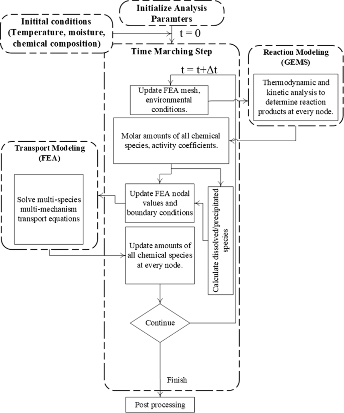
Adapted from [25]
Coupled reactive-transport modelling time-marching algorithm. Transport equations are solved using the finite element analysis (FEA) while the thermodynamic calculations are done using GEMS3K.
- 2.
Reactive-transport modelling using thermodynamically determined reaction isotherms In this approach, instead of fully coupling the transport and reactive processes in a time marching algorithm thermodynamic modelling is used to determine the reaction (i.e., binding) isotherms to eliminate the need to obtain them experimentally. Such an application of this approach, applied to chloride binding, was demonstrated in detail by Azad and Isgor [34]. One disadvantage of this approach is the need to calculate the isotherms at different temperatures if the temperature distribution in concrete varies spatially and temporally. An example is provided for developing chloride binding isotherms in the case studies.

In both approaches, some assumptions are needed for thermodynamic modelling. Although kinetic models for OPC hydration are available [59, 65], the kinetics of the SCM reactions are poorly understood. Further research is needed in this area as the authors are not aware of a viable kinetic model for SCM reactivity in concrete. As a result, the reactivity of the SCMs should either be estimated or measure experimentally [84]. The other issue originates from the current lack of understanding on how the hydrated phases interact (e.g., absorb and react) with chlorides. As discussed earlier, there is evidence for monosulfates binding chlorides; however, kinetics of this process is still not well understood. Therefore, until this understanding is further developed, some educated assumptions are needed regarding how much hydrated phases can chemically bind chlorides.
3 Numerical examples
3.1 Theoretical pore solution resistivity calculations
The calculation of pore solution resistivity is necessary for the determination of formation factor of concrete, which is used in the calculations of transport properties such as the effective ionic diffusion coefficients. In this numerical example, we show a comparison between the theoretical determination of pore solution resistivity using the NIST model and thermodynamic calculations. Ongoing research is aimed at comparing these models with measured pore solution compositions and electrical resisistivies. For this purpose, paste mixtures prepared with different cementitious materials and water-binder ratios were compared with the modelling predictions. Table 2 provides the chemical compositions of the cementitious materials used for the base cases. Three different mixtures (100% OPC, 60% OPC + 40% Slag, and 75% OPC + 25% fly ash) were investigated at three levels of w/cm (0.4, 0.45, 0.50). For comparison purposes all simulations were run at full hydration and under sealed curing conditions.
Figure 3 illustrates the differences between theoretically calculated concrete resistivities using the NIST model and thermodynamic (GEMS) calculations. The figure shows that both approaches provide comparable resistivites for the 100% OPC and fly ash blended mixtures. The NIST method provides higher resistivities than the thermodynamic approach for slag blended mixtures. While the reasons for this difference are still not clear, ongoing research (Montanari et al. in progress) has identified that mixtures composed of OPC and slag have a greater variation from the NIST model that other binder systems. Currently analysis appears to indicate that this is due to differences associated with higher alkali solubility in the mixtures with the slag; however, ongoing research is working to clarify the causes for this discrepancy. It can also be noted that the NIST model appears to illustrate a greater influence of the water-to cementitious ratio on the pore solution resistivity than the GEMS model (it should be noted that these differences are relatively small). Again, the reasons for this difference are still being investigated and compared with experimental observations.

Comparison of concrete resistivities calculated theoretically using the NIST model and thermodynamic calculations
3.2 Chloride binding isotherms: experimental versus theoretical
In this case study, we present the approach proposed by Jafari et al. [34] to compare thermodynamic calculations for chloride binding with experimental data from Zibara [35] who studied the binding of external chlorides by cement pastes. Three cementitious systems were selected for comparison: 100% OPC, 60% OPC + 40% slag, and 60% OPC + 40% FA. The mixtures had a w/b of 0.30 with a binder content of 450 kg/m3, matching their experimental counterparts. The chemical compositions of the cementitious materials are provided in Table 1. The salts in the form of 3 M NaCl was assumed to be introduced to the hardened cementitious matrix externally after 56 days from initial mixing, which corresponds to a degree of hydration of 70% (for w/b = 0.30) [36]. Isothermal conditions (23 °C) were assumed. For blended systems the reactivity for fly ash and slag were assumed to be 15% and 35%, respectively, in agreement with reactivity values for similar SCM compositions in pastes with low w/b (e.g., 0.30) [34]. It was assumed that all unhydrated binder was available for chloride binding, while only 15% of the reactive hydrated phases (i.e., AFm) was assumed to be reactive with salt, as suggested in an earlier work [34]. We acknowledge that availability of all unhydrated phases to chlorides might result in overestimation of binding, particularly at low chloride concentrations. Similarly, there is limited information on binding kinetics of hydrated phases. Research on both topics are needed for more accurate thermodynamic calculations.
Figure 4 illustrates the comparison of the thermodynamically calculated chloride binding with experimental data. The figure also shows the comparison of the binding isotherms that are determined experimentally and using thermodynamic modelling. It can be observed that in all mixtures, the thermodynamically calculated free/bound chlorides and their binding isotherms, are comparable to the experimentally determined counterparts. For the 100% OPC case, the two approaches are in in good agreement at all chloride levels, as shown in Fig. 4a. For the slag and fly ash blended systems (Fig. 4b, c, respectively), thermodynamic calculations over-predict the chloride binding at high chloride concentrations. This is mainly due to the fact that SCM-blended systems have larger aluminium content than OPC-based systems, leading to the formation of a larger AFm phase. Since we assumed that only 15% of the AFm phase is available for binding without any consideration of kinetics, chloride binding is likely overestimated in the SCM-blended systems. Furthermore, thermodynamic modelling calculates reactions at equilibrium conditions and does not consider the kinetics of these reactions. It is possible that some of the chloride binding reactions are rather slow and cannot be captured experimentally at the time of the testing. Until kinetic data are incorporated into thermodynamic modelling calculations, it is expected that there will be differences in theoretically calculated and experimentally calculated chloride binding, particularly for systems containing SCMs. It should also be remembered that in blended systems we have an increased degree of uncertainty associated with the reactivity of the SCMs used in the mixtures. As stated earlier, we assumed the reactivity for fly ash and slag were assumed to be 15% and 35%, respectively. However, we know that the reactivity of SCMs show a high degree of variability. For example, reactivity of fly ash can be relatively low (typically ranging from 10 to 50%) and they can vary considerably between sources [85]. Reported reactivity values for slag are larger (typically from 35 to 75%), but they also cover a large range [86]. Therefore, the effects of the limited SCM reactivity on chloride binding and the composition of concrete pore solution cannot be ignored. Regardless of all these differences, the thermodynamically calculated binding isotherms provide reasonable substitute for the empirically determined chloride binding and enables incorporation of binding reactions to modelling exercise without the need for empirical data.

Comparison of the thermodynamically calculated chloride binding with experimental data
In recent years, several attempts have been made to standardize the SCM reactivity tests [87,88,89,90,91]. These tests are limited for use as a standard for quantifying fly ash reactivity and do not provide a simple numerical result for the maximum reactivity of the pozzolan [89]. Recently, a method for determining SCM reactivity has been proposed to overcome this issue [84]. The method provides a single value for reactivity, which can be used in modelling exercises such as the one presented here. Accurate determination of SCM reactivity will lead to more accurate modelling of chloride binding, and all other SCM reactions, using thermodynamic modelling. It should also be acknowledged that the assumptions on the percentages of hydrated phases available for reaction are not necessarily unique. This problem originates from the fact that there is controversy on how much of the hydrated products are available for chloride binding. More research is needed on this issue so that the proposed modelling approach can be used more effectively.
3.3 Reactive-transport modelling
In this numerical example, we demonstrate the use of the modelling framework to model reactive-transport processes in concrete with only saturated concrete resistivity at a reference age and temperature as the measured quantity as input. The simulations were carried out on the base case OPC cement showing in Table 2, with some variations in C3A content to vary the chloride binding capacity. Concrete with w/cm of 0.45 and at 90% degree of hydration was simulated. Simulations were performed on 250 mm thick a concrete slab that is continuously ponded with 3.5% (600 mol/m3 solution) NaCl solution. Chloride binding was modelled using thermodynamic calculations following the same assumptions made in the previous numerical example. Transport properties were calculated using the formation factor of concrete that is computed from the measured concrete resistivity and thermodynamically calculated pore solution resistivity. In order to simplify the presentation and comparison of the results presented in this paper, isothermal conditions were considered. Transport equations were solved using the finite element method; thermodynamic calculations were made using GEMS3K. A summary of the analysis parameters are provided in Table 3. Since the model parameters are described earlier, they are not repeated here.
Selected results of the analysis cases are presented in Figs. 5 and 6. Note that the results are presented in terms of ionic activities instead of concentrations to reflect the effect of ionic strength and chemical activity on transport. Figure 5 shows the effect of measured concrete resistivity and chloride binding on the activity of chlorides in the concrete pore solution as a function of concrete depth after 10 years of continuous salt ponding. As it can be observed from the comparison of Fig. 5a–c, increased measurement of concrete resistivity, hence increased formation factor, results in slower ingress of chloride ions in the concrete. Also shown in Fig. 5 is the effect of thermodynamically calculated chloride binding on the chloride profiles. As expected, the effect of increased levels of C3A content in cement, increase chloride binding. Figure 6 shows the variation of other ionic species in concrete after 10 years of salt exposure as a function of depth. For clarity, these results are shown only for the moderate chloride binding cases (C3A = 7.5%). The effect of measured resistivity is also clear in these results (shown in captions). These simulations can be refined further as we develop our understanding on reaction kinetics of cementitious systems that could supplement thermodynamic calculations as well as reactivity of SCMs.

The comparison of activities of chloride ions in OPC concrete (w/cm = 0.45) with different chloride binding capacities and concrete resistivities of a 7.3 \(\Omega\)-m, b 18.3 \(\Omega\)-m, and c 36.6 \(\Omega\)-m. The base chemical composition of the OPC is given in Table 2. The results are shown for 10 years of continuous salt exposure

The comparison of activities of other ionic species in OPC concrete (w/cm = 0.45; C3A = 7.5%) for different measured concrete resistivities of a 7.3 \(\Omega\)-m, b 18.3 \(\Omega\)-m, and c 36.6 \(\Omega\)-m. The base chemical composition of the OPC is given in Table 2. The results are shown for 10 years of continuous salt exposure
4 Summary
This paper described a framework for a reactive-transport model beginning with governing equations. The paper then described the determination of the formation factor using the pore solution composition from thermodynamic calculations. The pore solution resistivity predicted by the thermodynamics model here was compared with the NIST model and a reasonable comparison was observed for the OPC and OPC-Fly Ash system; however, the NIST model showed higher resistivities for OPC-slag systems. The paper also used the thermodynamic model to estimate chloride binding reactions and chloride binding isotherms. The thermodynamically calculated binding isotherms are comparable to the experimentally determined counterparts for the 100% OPC case; however, thermodynamic calculations over-predict binding at high chloride concentrations for the slag and fly ash blended systems. This is likely due to the fact that thermodynamic modelling calculates reactions at equilibrium conditions and does not consider the kinetics of these reactions. The measured electrical resistivity is normalized by the pore solution resistivity to compute the formation factor which is used in the solution of the reactive-transport equations to assess ionic movement, chloride ingress and binding. The presentation of the model will undoubtedly require comparison with experimental data and further refinement; however, it does present a potential approach that can complement field testing for use in concrete specifications. The proposed framework can be refined further as we develop our understanding on reaction kinetics of cementitious systems that could supplement thermodynamic calculations as well as reactivity of SCMs.
Change history
12 December 2019
The article, A nearly self-sufficient framework for modelling reactive-transport processes in concrete, written by O. Burkan Isgor and W. Jason Weiss, was originally published electronically on the publisher’s Internet portal (currently SpringerLink) on 28 December 2018 without open access.
References
Wittmann F (1997) 50 years of experience in the service of building materials and structures. RILEM, Bagneux
Hansen TC (1974) Materials science and materials engineering education. Mater Constr 7(2):87–94
Gjørv OD (1969) Durability of reinforced concrete wharves in Norwegian harbours. Mater Constr 2(6):467–476
Valenta O (1970) From the 2nd RILEM symposium durability of concrete—in Prague. Mater Constr 3(4):333–345
AASHTO (2017) AASHTO PP-84-17—standard practice for developing performance engineered concrete pavement mixtures. American Association of State and Highway Transportation Official, Washington, DC
Azad VJ, Erbektas AR, Qiao C, Isgor OB, Weiss WJ (2018) Relating the formation factor and chloride binding parameters to the apparent chloride diffusion coefficient of concrete. ASCE J Mater Civ Eng. https://doi.org/10.1061/(ASCE)MT.1943-5533.0002615
Moradllo MK, Qiao C, Isgor OB, Weiss WJ (2018) Relating formation factor of concrete to water absorption. ACI Mater J. https://doi.org/10.14359/51706844
Radlinska A, Weiss J (2012) Toward the development of a performance-related specification for concrete shrinkage. J Mater Civ Eng 24(1):64–71
Suraneni P, Azad VJ, Isgor OB, Weiss WJ (2017) Concrete paving mixture compositions that minimize deicing salt damage. Transp Res Rec 2629:24–32
Todak H, Lucero C, Weiss WJ (2015) Why is the air there? Thinking about freeze-thaw in terms of saturation. Concr inFocus 27–33
Weiss WJ, Barrett TJ, Qiao C, Todak H (2016) Toward a specification for transport properties of concrete based on the formation factor of a sealed specimen. Adv Civ Eng Mater 5(1):179–194
Qiao C, Coyle A, Isgor OB, Weiss WJ (2018) Prediction of chloride ingress in saturated concrete using formation factor and chloride binding isotherm. Adv Civ Eng Mater 7:206–220
Suraneni P, Azad VJ, Isgor OB, Weiss J (2018) Role of supplementary cementitious material type in the mitigation of calcium oxychloride formation in cementitious pastes. J Mater Civ Eng 30(10):04018248
Suraneni P, Azad VJ, Isgor OB, Weiss WJ (2017) Use of fly ash to minimize deicing salt damage in concrete pavements. Transp Res Record 2629:24–32
Li WT, Pour-Ghaz M, Castro J, Weiss J (2012) Water absorption and critical degree of saturation relating to freeze-thaw damage in concrete pavement joints. J Mater Civ Eng 24(3):299–307
Pommersheim J, Clifton J (1985) Prediction of concrete service-life. Mater Struct 18(1):21–30
Page CL, Havdahl J (1985) Electrochemical monitoring of corrosion of steel in microsilica cement pastes. Mater Struct 18(1):41–47
Müller KF (1985) The possibility of evolving a theory for predicting the service life of reinforced concrete structures. Mater Struct 18(6):463–472
Page CL, Lambert P, Vassie PRW (1991) Investigations of reinforcement corrosion. 1. The pore electrolyte phase in chloride-contaminated concrete. Mater Struct 24(142):243–252
Garboczi EJ (1993) Computational materials science of cement-based materials. Mater Struct 26(158):191–195
Andrade C, Whiting D (1996) A comparison of chloride ion diffusion coefficients derived from concentration gradients and non-steady state accelerated ionic migration. Mater Struct 29(192):476–484
Marchand J (2001) Modeling the behavior of unsaturated cement systems exposed to aggressive chemical environments. Mater Struct 34(238):195–200
Quenard DA, Xu K, Kunzel HM, Bentz DP, Martys NS (1998) Microstructure and transport properties of porous building materials. Mater Struct 31(209):317–324
Samson E, Marchand J (2007) Modeling the transport of ions in unsaturated cement-based materials. Comput Struct 85(23–24):1740–1756
Azad VJ, Li C, Verba C, Ideker JH, Isgor OB (2016) A COMSOL-GEMS interface for modeling coupled reactive-transport geochemical processes. Comput Geosci 92:79–89
Karadakis K, Azad VJ, Ghods P, Isgor OB (2016) Numerical investigation of the role of mill scale crevices on the corrosion initiation of carbon steel reinforcement in concrete. J Electrochem Soc 163(6):C306–C315
Davies C (1967) Electrochemistry. Newnes, London
Samson E, Marchand J, Robert JL, Bournzel JP (1999) Modelling ion diffusion mechanisms in porous media. Int J Numer Meth Eng 46(12):2043–2060
Samson E, Marchand J (1999) Numerical solution of the extended Nernst–Planck model. J Colloid Interface Sci 215(1):1–8
Adamson AW, Gast AP (1997) Physical chemistry of surfaces, vol 6. Wiley InterScience, New York
Dean JA (1999) Lange’s handbook of chemistry, vol 15. McGraw-Hill, New York
Boddy A, Bentz E, Thomas MDA, Hooton RD (1999) An overview and sensitivity study of a multimechanistic chloride transport model. Cem Concr Res 29(6):827–837
Samson E, Marchand J (2007) Modeling the effect of temperature on ionic transport in cementitious materials. Cem Concr Res 37(3):455–468
Azad VJ, Isgor OB (2017) Modeling chloride ingress in concrete with thermodynamically calculated chemical binding. Int J Adv Eng Sci Appl Math 9(2):18–97
Rajibipour F (2006) In situ electrical sensing and material health monitoring in concrete structures. Purdue University, West Lafayyete
Weiss WJ, Spragg RP, Isgor OB, Ley MT, Van Dam T (2018) Toward performance specifications for concrete: linking resistivity, RCPT and diffusion predictions using the formation factor for use in specifications. In: High tech concrete: where technology and engineering meet. Springer, pp 2057–2065
AASHTO (2015) AASHTO TP 119—standard method of test for electrical resistivity of a concrete cylinder tested in a uniaxial resistance test. American Association of State and Highway Transportation Officials, Washington, DC
AASHTO (2017) AASHTO T 358—Standard method of test for surface resistivity indication of concrete’s ability to resist chloride ion penetration. American Association of State Highway and Transportation Officials, Washington, DC
Spragg R, Villani C, Snyder K, Bentz DP, Bullard JW, Weiss WJ (2013) Factors that influence electrical resistivity measurements in cementitious systems. Transp Res Record 2342:90–98
Spragg R, Jones S, Bu Y, Lu Y, Bentz D, Snyder K, Weiss J (2017) Leaching of conductive species: implications to measurements of electrical resistivity. Cem Concr Compos 79:94–105
Spragg R, Villani C, Weiss WJ (2016) Electrical properties of cementitious systems: formation factor determination and the influence of conditioning procedures. Adv Civ Eng Mater 5(1):124–148
Bentz DP (2007) A virtual rapid chloride permeability test. Cem Concr Compos 29(10):723–731
Weiss J, Snyder K, Bullard J, Bentz D (2013) Using a saturation function to interpret the electrical properties of partially saturated concrete. J Mater Civ Eng 25(8):1097–1106. https://doi.org/10.1061/(Asce)Mt.1943-5533.0000549
Salehi M, Ghods P, Isgor OB (2015) Numerical study on the effect of cracking on surface resistivity of plain and reinforced concrete elements. J Mater Civ Eng 27(12):04015053
Salehi M, Ghods P, Isgor OB (2016) Numerical investigation of the role of embedded reinforcement mesh on electrical resistivity measurements of concrete using the Wenner probe technique. Mater Struct 49(1–2):301–316
Glosser D, Azad VJ, Suraneni P, Isgor OB, Weiss WJ (2019) An extension of the Poers–Brownyard model to pastes containing SCM. ACI Mater J (in press)
Azad VJ, Suraneni P, Isgor OB, Weiss WJ (2017) Interpreting the pore structure of hydrating cement phases through a synergistic use of the Powers–Brownyard model, hydration kinetics, and thermodynamic calculations. Adv Civ Eng Mater 6(1):1–16
Chang MT, Montanari L, Suraneni PWWJ (2018) Expression of cementitious pore solution and the analysis of its chemical composition and resistivity using X-ray fluorescence. J Vis Exp. https://doi.org/10.3791/58432
Snyder KA, Feng X, Keen BD, Mason TO (2003) Estimating the electrical conductivity of cement paste pore solutions from OH−, K+ and Na+ concentrations. Cem Concr Res 33(6):793–798
Lothenbach B, Matschei T, Möschner G, Glasser FP (2008) Thermodynamic modelling of the effect of temperature on the hydration and porosity of Portland cement. Cem Concr Res 38(1):1–18
Kulik DA, Wagner T, Dmytrieva SV, Kosakowski G, Hingerl FF, Chudnenko KV, Berner UR (2012) GEM-Selektor geochemical modeling package: revised algorithm and GEMS3 K numerical kernel for coupled simulation codes. Comput Geosci. https://doi.org/10.1007/s10596-012-9310-6
Dilnesa B, Lothenbach B, Le Saout G, Renaudin G, Mesbah A, Filinchuk Y, Wichser A, Wieland E (2011) Iron in carbonate containing AFm phases. Cem Concr Res 41(3):311–323
Dilnesa BZ, Lothenbach B, Renaudin G, Wichser A, Kulik D (2014) Synthesis and characterization of hydrogarnet Ca3 (Alx Fe1−x)2 (SiO4)y(OH)4(3−y). Cem Concr Res 59:96–111
Dilnesa BZ, Lothenbach B, Renaudin G, Wichser A, Wieland E (2012) Stability of monosulfate in the presence of iron. J Am Ceram Soc 95(10):3305–3316
Kulik DA (2011) Improving the structural consistency of C–S–H solid solution thermodynamic models. Cem Concr Res 41(5):477–495. https://doi.org/10.1016/j.cemconres.2011.01.012
Kulik DA, Kersten M (2001) Aqueous solubility diagrams for cementitious waste stabilization systems: II, end-member stoichiometries of ideal calcium silicate hydrate solid solutions. J Am Ceram Soc 84(12):3017–3026
Kulik DA, Kersten M (2002) Aqueous solubility diagrams for cementitious waste stabilization systems. 4. A carbonation model for Zn-doped calcium silicate hydrate by Gibbs energy minimization. Environ Sci Technol 36(13):2926–2931
Lothenbach B, Matschei T, Moschner G, Glasser FP (2008) Thermodynamic modelling of the effect of temperature on the hydration and porosity of Portland cement. Cem Concr Res 38(1):1–18. https://doi.org/10.1016/j.cemconres.2007.08.017
Lothenbach B, Winnefeld F (2006) Thermodynamic modelling of the hydration of Portland cement. Cem Concr Res 36(2):209–226. https://doi.org/10.1016/j.cemconres.2005.03.001
Lothenbach B, Pelletier-Chaignat L, Winnefeld F (2012) Stability in the system CaO–Al2O3–H2O. Cem Concr Res 42(12):1621–1634. https://doi.org/10.1016/j.cemconres.2012.09.002
Matschei T, Lothenbach B, Glasser FP (2007) Thermodynamic properties of Portland cement hydrates in the system CaO–Al2O3–SiO2–CaSO4–CaCO3–H2O. Cem Concr Res 37(10):1379–1410. https://doi.org/10.1016/j.cemconres.2007.06.002
Moschner G, Lothenbach B, Rose J, Ulrich A, Figi R, Kretzschmar R (2008) Solubility of Fe-ettringite (Ca6[Fe(OH)6]2(SO4)3·26H2O). Geochim Cosmochim Acta 72(1):1–18. https://doi.org/10.1016/j.gca.2007.09.035
Moschner G, Lothenbach B, Winnefeld F, Ulrich A, Figi R, Kretzschmar R (2009) Solid solution between Al-ettringite and Fe-ettringite (Ca6[Al1−xFex(OH)(6)](2)(SO4)(3) 26H(2)O). Cem Concr Res 39(6):482–489. https://doi.org/10.1016/j.cemconres.2009.03.001
Schmidt T, Lothenbach B, Romer M, Scrivener K, Rentsch D, Figi R (2008) A thermodynamic and experimental study of the conditions of thaumasite formation. Cem Concr Res 38(3):337–349
Parrot L, Killoh D (1984) Prediction of cement hydration. Br Ceram Proc 35:41–53
Hong SY, Glasser FP (1999) Alkali binding in cement pastes Part I. The C–S–H phase. Cem Concr Res 29(12):1893–1903
Azad VJ, Isgor OB (2016) A thermodynamic perspective on chloride limits of concrete produced with SCMs. ACI Spec Publ Chloride Limits Thresholds Concr Contain Suppl Cem Mater (in press)
Ji G, Isgor OB (2007) Effects of Tafel slope, exchange current density and electrode potential on the corrosion of steel in concrete. Mater Corros 58(8):573–582. https://doi.org/10.1002/maco.200604043
Isgor OB, Razaqpur AG (2006) Modelling steel corrosion in concrete structures. Mater Struct 39(3):291–302. https://doi.org/10.1617/s11527-005-9022-7
Kranc SC, Sagues AA (2001) Detailed modeling of corrosion macrocells on steel reinforcing in concrete. Corros Sci 43(7):1355–1372. https://doi.org/10.1016/S0010-938x(00)00158-X
Florea MVA, Brouwers HJH (2012) Chloride binding related to hydration products Part I: Ordinary Portland Cement. Cem Concr Res 42(2):282–290
Yuan Q, Shi CJ, De Schutter G, Audenaert K, Deng DH (2009) Chloride binding of cement-based materials subjected to external chloride environment—a review. Constr Build Mater 23(1):1–13
Martin-Perez B, Zibara H, Hooton RD, Thomas MDA (2000) A study of the effect of chloride binding on service life predictions. Cem Concr Res 30(8):1215–1223
Nilsson LO, Massat M, Tang L (1994) The effect of non-linear chloride binding on the prediction of chloride penetration into concrete structutres. In: Malhotra VM (ed) Durability of concrete. American Concrete Institute (ACI), Detroit, pp 469–486
Tang LP, Nilsson LO (1993) Chloride binding-capacity and binding isotherms of OPC pastes and mortars. Cem Concr Res 23(2):247–253
Tran VQ, Soive A, Baroghel-Bouny V (2018) Modelisation of chloride reactive transport in concrete including thermodynamic equilibrium, kinetic control and surface complexation. Cem Concr Res 110:70–85
Kulik DA, Wagner T, Dmytrieva SV, Kosakowski G, Hingerl FF, Chudnenko KV, Berner UR (2013) GEM-Selektor geochemical modeling package: revised algorithm and GEMS3 K numerical kernel for coupled simulation codes. Comput Geosci 17(1):1–24. https://doi.org/10.1007/s10596-012-9310-6
Wagner T, Kulik DA, Hingerl FF, Dmytrieva SV (2012) Gem-Selektor geochemical modeling package: TSolmod library and data interface for multicomponent phase models. Can Mineral 50(5):1173–1195. https://doi.org/10.3749/canmin.50.5.1173
Kulik D, Berner U, Curti E (2004) Modelling chemical equilibrium partitioning with the GEMS-PSI code. In: Smith B, Gschwend B (eds) PSI scientific report 2003/Volume IV. Nuclear energy and safety, Paul Scherrer Institute, Villigen, Switzerland, pp 109–122
Kulik DA (2002) Gibbs energy minimization approach to modeling sorption equilibria at the mineral-water interface: thermodynamic relations for multi-site-surface complexation. Am J Sci 302(3):227–279. https://doi.org/10.2475/ajs.302.3.227
Johnson JW, Oelkers EH, Helgeson HC (1992) SUPCRT92: a software package for calculating the standard molal thermodynamic properties of minerals, gases, aqueous species, and reactions from 1 to 5000 bar and 0 to 1000 °C. Comput Geosci 18(7):899–947
Hummel W, Berner U, Curti E, Pearson F, Thoenen T (2002) Nagra/PSI chemical thermodynamic data base 01/01. Radiochim Acta 90(9–11/2002):805–813
Loser R, Lothenbach B, Leemann A, Tuchschmid M (2010) Chloride resistance of concrete and its binding capacity—comparison between experimental results and thermodynamic modeling. Cem Concr Compos 32(1):34–42
Suraneni P, Weiss J (2017) Examining the pozzolanicity of supplementary cementitious materials using isothermal calorimetry and thermogravimetric analysis. Cem Concr Compos 83:273–278. https://doi.org/10.1016/j.cemconcomp.2017.07.009
Zeng Q, Li KF, Fen-chong T, Dangla P (2012) Determination of cement hydration and pozzolanic reaction extents for fly-ash cement pastes. Constr Build Mater 27(1):560–569
Kocaba V, Gallucci E, Scrivener KL (2012) Methods for determination of degree of reaction of slag in blended cement pastes. Cem Concr Res 42(3):511–525
Avet F, Snellings R, Diaz AA, Ben Haha M, Scrivener K (2016) Development of a new rapid, relevant and reliable (R-3) test method to evaluate the pozzolanic reactivity of calcined kaolinitic clays. Cem Concr Res 85:1–11
Donatello S, Tyrer M, Cheeseman CR (2010) Comparison of test methods to assess pozzolanic activity. Cem Concr Compos 32(2):121–127
Snellings R, Scrivener KL (2016) Rapid screening tests for supplementary cementitious materials: past and future. Mater Struct 49(8):3265–3279
Taylor-Lange SC, Riding KA, Juenger MCG (2012) Increasing the reactivity of metakaolin-cement blends using zinc oxide. Cem Concr Compos 34(7):835–847
Tironi A, Trezza MA, Scian AN, Irassar EF (2013) Assessment of pozzolanic activity of different calcined clays. Cem Concr Compos 37:319–327
Barde V, Radlinska A, Cohen M, Weiss WJ (2009) Relating material properties to exposure conditions for predicting service life in concrete bridge decks in Indiana. Publication FHWA/IN/JTRP-2007/27. Joint Transportation Research Program, Indiana Department of Transportation and Purdue University, West Lafayette, Indiana
Acknowledgements
Authors would like to acknowledge the financial support provided by their endowed faculty positions, namely, The Miles Lowell and Margaret Watt Edwards Distinguished Chair in Engineering, and John and Jean Loosely Faculty Fellow. The authors would like to acknowledge Dr. Vahid Jafari Azad for his contributions to the reactive-transport modelling framework presented in this paper, Dr. Qiao Chunyu for his contributions to the development of relationships between formation factor and transport properties in concrete, Luca Montanari for his work on the resistivity of concrete pore solutions, and Dr. Hossein DorMohammadi for his help in performing some of the transport simulations presented in this paper.
Author information
Authors and Affiliations
Corresponding author
Ethics declarations
Conflict of interest
The authors declare that they have no conflict of interest.
Rights and permissions
Open Access This article is distributed under the terms of the Creative Commons Attribution 4.0 International License (http://creativecommons.org/licenses/by/4.0/), which permits use, duplication, adaptation, distribution and reproduction in any medium or format, as long as you give appropriate credit to the original author(s) and the source, provide a link to the Creative Commons license and indicate if changes were made.
About this article

Cite this article
Isgor, O.B., Weiss, W.J. A nearly self-sufficient framework for modelling reactive-transport processes in concrete. Mater Struct 52, 3 (2019). https://doi.org/10.1617/s11527-018-1305-x
Received:
Accepted:
Published:
DOI: https://doi.org/10.1617/s11527-018-1305-x