
. Introduction
Radiometric dating of a building by stimulated luminescence is currently based on the chronology obtained through Thermoluminescence (TL) and/or Optically Stimulated Luminescence (OSL) dating of bricks (Goedicke et al., 1981; Bailiff and Holland, 2000; Martini and Sibilia, 2001; Bailiff, 2007; Guibert et al., 2009a; Stella et al., 2014). These procedures are based on the assumption that the manufacture of the bricks happened almost contemporary to, or not much earlier than, its use. This represents an evident limitation of the method, especially when the studied building has a complex history of construction/modification phases through time. In fact, TL dating of bricks can fail to identify the period of construction and/or successive modifications of buildings if older materials were reused. To overcome this issue, studies on the possibility of dating several types of historical mortars (mainly lime and mud mortars) through optically stimulated techniques (OSL) have been developed (Zacharias et al., 2002; Feathers et al., 2008; Gueli et al., 2010; Goedicke, 2011; Stella et al., 2013; Guibert et al.,2017). The possibility to use mortars to evaluate the time of construction, repair works or modifications of a structure represents an important break-through in dating historical buildings. The natural dosimeter is quartz in the sand fraction and/or in the fine grain fraction (Gueli et al., 2010; Stella et al., 2013) of these materials and the zero event can be related to exposure to daylight during construction, i.e. the mixing and laying of the mortar. However, the choice of granulometry extracted from inert is strongly influenced by the characteristics of the mortar and the available quantity because, in order to obtain as possible accurate and precise data, several dosimeters control and measurements must be carried out. Still, relative errors below 5% cannot be reached through OSL dating, due to different intrinsic and extrinsic factors (water content evaluation, beta and gamma microdosimetry, bleaching degree, complex entourage…) (Feathers et al., 2008; Goedicke, 2011; Stella et al., 2013; Panzeri, 2013; Urbanová et al., 2015). The evaluation of bleaching degree related to the granulometry of the extracted and measured quartz has been studied in recent years. The more recent studies on mortar dating demonstrate that mortar aggregate can contain a sufficient number of well-bleached quartz grains and this represents a real potential for dating the mortar by Single Grain OSL (SG-OSL) (Urbanová et al., 2015, 2016; Guibert et al., 2017).
Furthermore, Urbanová and Guibert (2017), with an interesting discussion and analysis about all the aspects of the sample preparation through specificity of the measurement protocol and data evaluation to the age estimation, highlight the importance of the material characterization before the SG-OSL analysis.
In the case of young buildings and/or with chronologically close construction phases, dating techniques, stratigraphic and historical assessments should be joined with other studies providing useful information on the composition and manufacture of the building materials, namely defining classes of materials and their specific uses or uses through time in the same structure.
In this context the present paper concerns the results of a multidisciplinary study regarding the chronology of the Convento de S. Francisco (St. Francis Convent, Coimbra, Portugal) construction phases established by different dating techniques (TL for bricks and OSL for lime mortars), stratigraphic information, compositional and color characterization of materials.
Based on the stratigraphic analysis of the building and considering chronological issues raised, regarding the construction sequence, the materials and sampling points were selected.
. Historical and archaeological survey
Located in Coimbra (Portugal), on the left bank of the Mondego River, the Convento de S. Francisco corresponds to a large compound of different built bodies, with two to three floors each, organized around a cloister. Built in the 17th century, the structure was occupied by the Franciscans until 1843, after which, and until mid-20th century, several factories were installed, with considerable impact on the main structure.
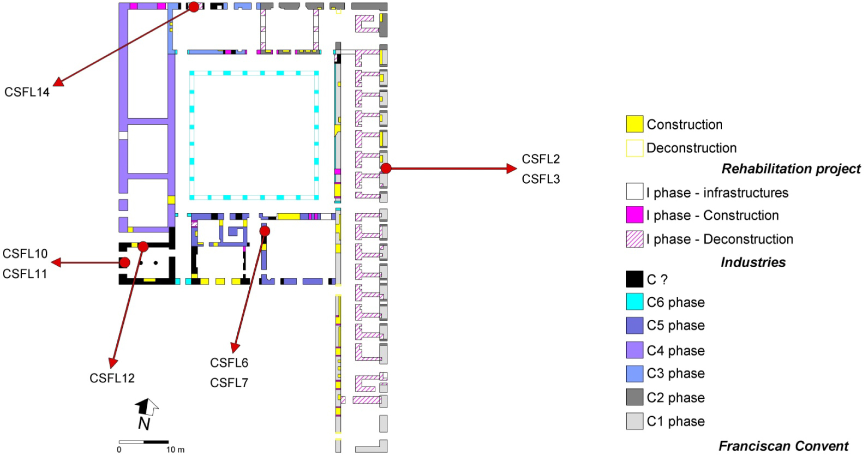
During the building rehabilitation project, a large scale Archaeology operation was implemented. Since all the building’s plasters had previously been removed, it was possible to observe and record a vast amount of stratigraphic information related to its construction process. Several observations are consistent with a phased construction, and allowed a preliminary framework for the buildings construction history. Thus, based on stratigraphic analysis, eight different construction phases were defined (Fig. 1): six related to the construction process of the convent throughout the Modern Age; one integrating all features related to its industrial occupations (19th/20th centuries); and lastly, one including transformations introduced by the recent rehabilitation project (21th century) (Almeida et al., 2011).
Fig. 1
Plan of the 2nd Floor of the Convento de São Francisco with construction phases and sampling points.
Concerning the convent’s construction throughout the Modern Age, besides documental information regarding the outset of the endeavour (1602), we have no evidence (documental, or other) allowing precise chronological assignment to the six different proposed construction phases. Furthermore, stratigraphic information solely was not enough to integrate several built elements within the overall sequence of the convent’s construction process. Hence, in order to test the possibility for dating different phases proposed and to surpass some defaults in the stratigraphic information, an initial program of dating and material characterization was designed.
The study included sampling material from built elements which (Fig. 1): were not clearly integrated in the construction sequence (CSFL2/CSFL3 and CSFL10/CSFL11); or, although well integrated in the construction sequence, would benefit from exact chronological integration (CSFL6 / CSFL7, CSFL12 and CSFL14).
Fig. 1 and Table 1 show the details for label, nature and sampling point for each sample.
Table 1
Details of the samples studied in this work with ID number, material and sampling point description.
| Sampling point (floor 2) | |||
|---|---|---|---|
| Sample | Material | Architectural element | Height1 (cm) |
| CSLF2 | Brick | Arc (east) | 350 |
| CSLF3 | Mortar | ||
| CSLF6 | Brick | Arc (south) | 80 |
| CSLF7 | Mortar | ||
| CSLF10 | Brick | Arc (west) | 235 |
| CSLF11 | Mortar | ||
| CSLF12 | Mortar | Wall (west) | 145 |
| CSLF14 | Mortar | Wall (north) | 150 |
. Luminescence dating
sample preparation
After a macroscopic description the mortar samples were divided into two parts: one part for luminescence dating and the other part for XRD measurements. The difficulty to extract pure coarse grain quartz fraction of sufficient quantity from sand used as inert in lime mortar has led the authors to study the luminescent emission from polymineral fine grain phase “enriched in quartz” through HF etching procedures during preparation phase of the samples (Prasad, 2000; Mauz and Lang, 2004; Stella et al., 2013). The possibility to use this procedure must be validate by several tests (e.g. preheating test, recovery test, thermal transfer test…). After the removal of two external millimetres, mortar samples were pretreated with 10% H2O2 for four days to remove organic material, and with 20% hydrochloric acid for 120 min. to dissolve carbonates. Subsequently the samples were treated with 20% HF at RT for 15 minutes, washed in 10% HCl for 25 minutes to remove fluorides, and then the 4–11 μm grain fraction enriched in quartz was selected and deposited onto 9.8 mm diameter discs (Gueli et al., 2010; Stella et al., 2013). The purity of fractions was then evaluated by the ratio between the post-IR OSL/T2 (normalized OSL intensity after IR stimulation) and OSL/T1 (normalized OSL emission) that resulted close to unity (Mauz and Lang, 2004; Prasad, 2000; Shen et al.,2007; Zhang and Zhou, 2007; Gueli et al., 2010; Gerardi et al., 2012; Stella et al., 2013).
For brick samples the polymineral fine grain fraction was obtained by PH3DRA standard procedure (Gueli et al., 2009, 2010; Guibert et al., 2009a). As for mortars, the outer two millimetre layer was removed, then the sample was crushed and sieved to select the fraction below 40 μm. Following, a sequence of etching procedures was made: 10% HCl for 1h to remove the carbonate, 10% H2O2 for 48 hours to remove the organic component, 1% HF for 1 hour to remove clay mineral, and 10% HCl for 25 minutes to eliminate fluorosilicates possibly formed. Through a sedimentation procedure, polymineral fine grain fraction in the 4–11 μm range was obtained and then deposited onto 9.8 mm diameter disc. In preparation lab, room lighting is provided by Illford DL10 lamps equipped with Ilford #902 filters.
Equipment
TL for bricks, OSL and IRSL (InfraRed Stimulated Luminescence) for mortars were performed using semi-automated Risø readers (TL-DA-10 and TL-DA-15) with EMI 9235QA photomultipliers (Bøtter-Jensen, 1997; Bøtter-Jensen et al., 2000). TL glow curves were recorded in the TL-DA-10 detection system using Corning 7-59 and Schott BG-12 optical filters. OSL and IRSL signals were obtained using a TL-DA-15 reader equipped, respectively, with 41 blue LEDs (470± 30 nm) and with a laser diode (830 ± 10 nm). The stimulation units delivered about 30 mWcm–2 for OSL and 240 mWcm–2 for IRSL at 90% power. Both OSL and IRSL emissions were detected using a Hoya U340 optical filter.
Artificial luminescence signals were induced by two different 90Sr-90Y calibrated beta sources integrated in the Risø systems delivering, respectively, 6 Gy/min in TL-DA-15 model used for mortars and 1.32 Gy/min in TL-DA-10 model used for bricks. 241Am calibrated alpha source delivering 2.7 Gy/min was used to evaluate the luminescence efficiency coefficient k (Tables 3 and 4) necessary to correct the alpha dose contribution to the annual dose (Aitken, 1985; Guibert et al., 2009a).
OSL measurements for mortars
For six aliquots of each sample ED measurements and recovery test as a function of preheating temperature (160–260°C) were made (Choi et al., 2003; Thomas et al., 2003; Kiyak and Canel, 2006; Stella et al., 2013). Each dose value was determined using the modified SAR protocol that provides the measure of the recuperated OSL signal following a zero Gy regenerative dose in a SAR measurement cycle (recuperation test). At the end of each measurements cycle, an optically stimulation for 40 s at 280°C allows hence to check if any thermal transfer of charge was occurred from levels insensitive to light to the OSL traps (Murray and Wintle, 2003).
After the SAR sequence, the same regeneration dose of the first point of beta irradiation is given again to check whether the sensitivity corrected OSL (LR/TR)/(L1/T1) is reproducible by the recycling ratio R. This value, moreover, identifies the presence of a possible systematic error in the interpolation of Ln/Tn onto the dose–response curves. On the same aliquots, the recovery test was performed. The cycle of SAR modified protocol was repeated 7 times using increasing regeneration doses from 0.5 to 7.5 Gy. For ED calculation, data are acceptable if the recovery test and recycling ratio are within ±10% of unity and recuperation test near to zero (Murray and Wintle, 2003). Being young samples, whose OSL signal is not dominated by the fast component, the integral signal of the first 0.4 s was used as OSL intensity, after subtraction of the background calculated from the following 0.4 s, for minimize the contribution from the medium and slow OSL signal components (Ballarini et al., 2007; Pawley et al., 2010; Gerardi et al., 2012). The uncertainties were quantified on the basis of statistical counting of luminescence signals and applying error propagation. Following the test dose, a cut heat of 160°C was applied. Table 2 shows the temperature range, where the ED has a constant value, and the preheating temperature value chosen for mortars dating. The individual ED values were entered into bins of 0.1 Gy and so the frequency distributions were obtained. Shapiro-Wilk normality test was used to determine if a data set is well-modeled by a normal distribution and to compute how likely it is for a random variable underlying the data set to be normally. The test rejects the hypothesis of normality when the p-value is less than or equal to 0.05. Failing the normality test allows you to state with 95% confidence the data does not fit the normal distribution.
Table 2
Plateau temperature range and preheating (Ph) temperature choose for ED evaluation.
| Sample | Plateau ED range (°C) | Ph temperature (°C) |
|---|---|---|
| CSLF3 | 180–220 | 200 |
| CSLF7 | 180–240 | 210 |
| CSLF11 | 180–220 | 200 |
| CSLF12 | 180–220 | 200 |
| CSLF14 | 180–240 | 210 |
For each sample passing no significant departure from normality was found. So, the frequency distributions were related with Gaussian fits (with standard deviations) and Mean ED values were obtained (Table 3). The results show a good degree of precision for equivalent dose results but in the case of fine grains deposited on discs, their high number (some thousands) will tend to average all signals proportionally to the inverse of the square root of the number of grains. This also implies the reduction of the dispersion between aliquots, so the deviation from a normal distribution is much less observable. The methodology used is then only indicative but not exhaustive to evaluate the bleaching degree of fine grains. In this case, the association between dates of bricks and dates of mortars coupled with historical and architectural survey represents an useful approach to obtain indications about the accuracy of the dating results.
Table 3
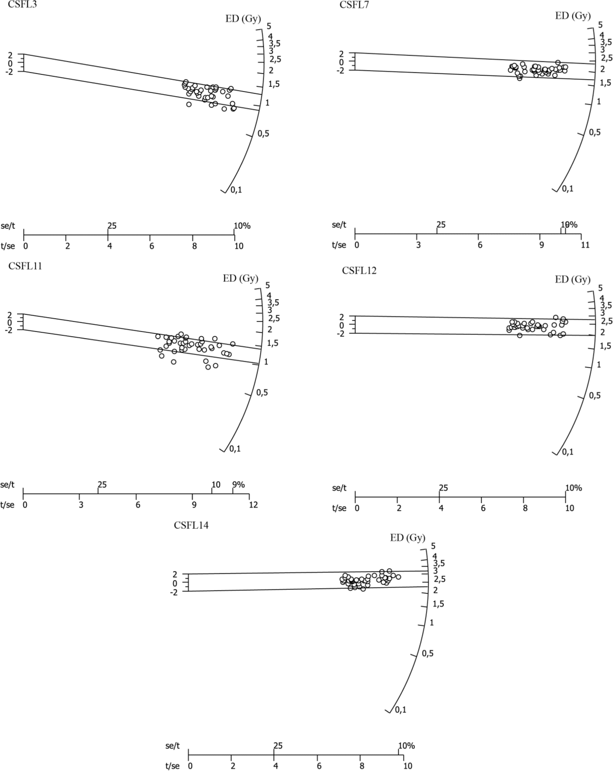
Number of aliquots (n), luminescence efficiency coefficient (k-value), Equivalent Dose (ED) Value and relative standard deviations (SD) obtained, respectively, by radial plot (ED Central Value, see Fig. 2) and from ED frequency distributions (Mean ED) for mortar samples.
| Sample | Number of aliquots (n) | k-value | ED Central Value*(Gy) SD | Mean ED**(Gy) SD |
|---|---|---|---|---|
| CSFL3 | 39 | 0.125 ± 0.010 | 1.17 0.10 | 1.18 0.18 |
| CSFL7 | 47 | 0.161 ± 0.012 | 2.03 0.21 | 2.02 0.26 |
| CSFL11 | 41 | 0.134 ± 0.010 | 1.13 0.11 | 1.12 0.17 |
| CSFL12 | 38 | 0.148 ± 0.010 | 2.41 0.15 | 2.42 0.22 |
| CSFL14 | 44 | 0.157 ± 0.010 | 2.61 0.18 | 2.63 0.25 |
The ED for age calculation was obtained by radial plots analysis (Galbraith et al., 1999; Stella et al., 2013) using RadialPlotter software (Vermeesch, 2009). Fig. 2 shows the radial plot of the dose distribution used to obtain the ED value for each mortar sample. In these graphs the position on the x-axis is a measure of the precision (t/se) with which ED is known. This axis is also expressed in terms of the relative error (se/t, expressed as a percentage). Table 3 reports for each mortar sample the number of aliquots, the k-value and the ED Central Value obtained by radial plot.
TL measurements for brick
The ED values for bricks were determined using TL measurements and especially the added dose method on the polymineral fine grain phase (Aitken, 1985; Guibert et al., 2009a). For each sample, 24 aliquots were prepared and grouped by six. The first group was used for measuring the natural TL signal. The remaining groups were serially and incrementally irradiated using a calibrated beta source. TL glow curves were recorded by heating the aliquots up to 500°C at a uniform heating rate of 5°C/s in an ultrapure nitrogen environment. The inter-aliquot intensity variations were corrected by second glow normalisation. Temperature region between 310 and 360°C TL (290–380°C plateau) was used for equivalent dose calculation (Qβ). In order to evaluate the possible nonlinearity behaviour of the sample at low artificial beta doses, qβ correction was determined from the intercept of the “second” growth curve behaviour. The same aliquots were then exposed to small and incrementing beta doses and a growth curve was constructed. The intercept of the curve on the dose axis is the correction value for supra-linear growth (qβ) (Aitken, 1985). ED was calculated adding Qβ and qβ values. From artificial luminescence signals induced by calibrated alpha doses the luminescence efficiency coefficient k was determined (Guibert et al., 2009a). All samples showed a growth linear luminescent behaviour vs. dose. For each sample measurements of luminescence loss over time were performed (Aitken,1985). The results obtained exclude the presence of anomalous fading. Table 4 shows k value, Qβ and qβvalue obtained for each brick sample.
Dose rate measurements
U, Th and K contents (Table 5) were determinate from high resolution gamma spectrometry measurements (HPGe) (Goedicke, 2011). The comparison between the activity of 238U (deduced from the 235U and 234Th gamma emissions) and that of 226Ra (deduced from 214Pb and 214Bi γ emissions in equilibrium with 222Rn) shows an equilibrium of the U-series (Table 5) (Guibert et al.,2009b). Annual dose components due to radioelements in both bricks and mortars were calculated from radioactive contents by conversion factors of Guérin et al. (2011).
Table 5
Radioactive measurements: Sample name, sample material with U, Th, K contents obtained by high gamma spectrometry and 238U/226Ra ratio.
The dose contributions of the sample were corrected on the basis of porosity factor (W) experimentally measured and of saturation factor (F) estimated on the basis of sampling point (height, inside or outside) (Aitken, 1985). In this particular case an F value of 0.3 ± 0.2 was considered. The annual environmental dose rate was measured using TL dosimeters (GR200A) enclosed in capsules placed in situ at the sampling points (Gueli et al., 2009; Stella et al., 2013) adding cosmic radiation calculated according to Prescott and Hutton (1988).
Table 6 shows the contributions to the annual dose for each sample: internal components Dαint and Dβint, corrected for water content, and the environmental contribution Denv.
Table 6
Contributions to the annual dose rate: Sample name, sample material, porosity factor W, alpha and beta internal dose rates (Dαint and Dβint) and environmental component (Denv).
Age Calculation
ED values obtained on the two FG brick and mortar samples were entered in the following age equation:
where ED is the equivalent dose, k is the alpha efficiency coefficient, Dα int, Dβ int and Denv are, respectively, the annual dose contributions, corrected with humidity and porosity factors (W, F), from the sample itself and from environment.
Table 7 shows, for each sample, the technique and the method used for ED determination, the annual dose rate, the ages and the corresponding AD dates obtained.
Table 7
Dating of samples: Sample name, sample material, technique, method with ED, annual dose rate, the individual dating results (referred to the year of the TL measurements) and the corresponding calendar dates obtained for both bricks and mortars.
. Composition and provenance
Samples preparation and equipment
Mineralogical characterization was based on X-ray diffraction (XRD) performed with a Philips X’Pert Pro PW3710 diffractometer equipped with a CuKα radiation, operating at 40 kV and 20 mA. Non-oriented aggregates of pulverized bulk material were measured between 2 and 60° using a step of 0.02° 2θ and 1.0 s scanning time in each step.
The macroscopic description of the mortars was performed in the laboratory after sampling. The mineralogical characterization of the mortars by XRD was performed later.
Contact spectrophotometry was used for colorimetric characterization of the mortars. The measurements were made with a portable Konica-Minolta CM2600D instrument, equipped with an integrating sphere in the geometry d/8° after the usual procedures for black and white adjustment, selecting an area of 11 mm diameter. Such measures are carried out directly in situ and are non-destructive. For this reason, no sample preparation was required.
Semi-quantitative analysis
After the qualitative interpretation of all the mineral constituents and taking into account the limitations imposed by the method, a semi-quantitative estimation was carried out in order to facilitate the mineralogical interpretation of the results. However it must be kept in mind that the percentages obtained should be only relative indicators of the concentration of the minerals and not absolute values since the associated error is high.
Semi-quantitative analyses were performed by measuring the areas of the peaks corresponding to the typical diffraction maxima spacings of each mineral divided by the respective reflector powers (Schultz, 1964; Moore and Reynolds, 1997; Thorez, 1976; Dias, 1998). The whole occurring phyllosilicates (total percentage) were determined by considering the main peak area at Bragg’s law interatomic spacing d=4.48 Å peak.
All the mineral associations of the analyzed mortar samples present, as essential minerals, a large proportion of quartz followed by calcite and K-feldspars, sometimes with similar values for both these minerals (Table 8, Fig. 3). For all samples, phyllosilicates, in particular clay minerals, as well as dolomite and Na-rich plagioclases are accessory minerals, with the exception of CSFL12 sample in which Na-rich plagioclases reached the 10%.
Table 8
XRD semi-quantitative mineralogical composition of mortars (%) and aggregate/binder ratio (Qz – quartz; K-felds – potassium feldspars; Na-plag – sodium plagioclases; Cal – calcite; Dolo – dolomite; Phyl – phyllossilicates; * – traces).
| Sample | Qz | K-felds | Na-plag | Cal | Dolo | Phyl | Aggregate (A) | Binder (B) | A/B Ratio |
|---|---|---|---|---|---|---|---|---|---|
| CSFL3 | 65 | 21 | 1 | 13 | * | * | 86 | 13 | 6.62 |
| CSFL7 | 65 | 5 | * | 26 | 2 | 2 | 70 | 26 | 2.69 |
| CSFL11 | 71 | 14 | 1 | 13 | 1 | * | 85 | 13 | 6.54 |
| CSFL12 | 59 | 12 | 10 | 18 | 1 | * | 71 | 18 | 3.94 |
| CSFL14 | 66 | 11 | 1 | 21 | 1 | * | 77 | 21 | 3.67 |
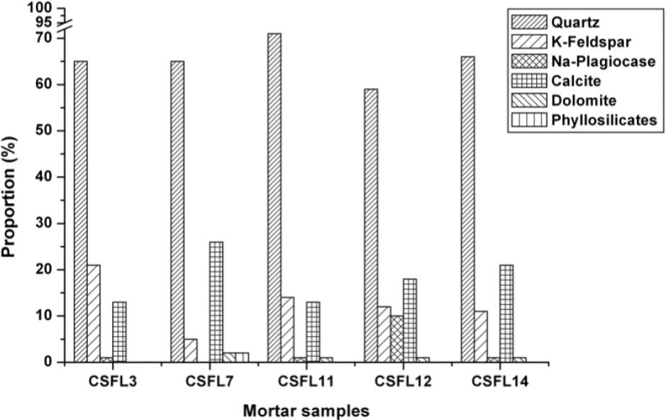
An initial macroscopic observation showed that mortar samples consist mainly of quartz as aggregate and carbonates as cement (binder). In all the analyzed samples the sum of quartz and K-feldspars reaches a mean above 75%. Since some carbonate aggregates (dolostone, dolomitic limestone and limestone fragments) were identified by macroscopic observation, the carbonate composition of the bulk mortar evaluated through XRD corresponds both to the aggregate and the lime paste from the binder, without discrimination. However those carbonate compounds should not influence the binder/aggregate ratio, since they are in a very low occurrence. Furthermore, in what concerns to the binder, this technique only provides the detection of crystalline phases resulting from carbonation and hardening of the original burned limestone that have produced the lime paste (Sanjurjo-Sánchez et al., 2010). Nevertheless, the proportions obtained by XRD semi-quantification confirm the assumption that the sum of Quartz and K-feldspars corresponds to the essential of the aggregate and calcite mostly to the binder (Table 8).
The quartz/K-feldspars ratio is always higher than three. Sample CSFL7 is different by having quartz reaching thirteen times the proportion of K-feldspars, higher proportions of carbonates and noteworthy quantities of phyllosilicates.
Morphometric and textural observations during the initial macroscopic analysis showed a large proportion of mostly subangular to angular silicate sand in all samples. All samples contain also aggregates of variable dimensions below the class of fine gravel, essentially less than 8 mm. Coupled with the XRD data, these characteristics points to a provenance of the aggregates from raw alluvium materials, probably those occurring in the left bank of the Mondego River, where the Convento de S. Francisco is located. The mineralogical composition of the CSFL7 sample is compatible with the same provenance, but with minor amount of carbonate clasts and detrital mica. Since the convent is also at the base of a dolomitic limestone hill, we can assume that a less selected alluvial/colluvial aggregate wasused.
The very scarce presence of phyllosilicates, in particular clay minerals, is remarkable and probably should be explained by the aggregate origin and the technology for the production of mortars. We can assume that raw materials sources were mainly nearby Mondego’s channel deposits comprising a low rate of clay particles, with the above commented exception of sample CSFL7.
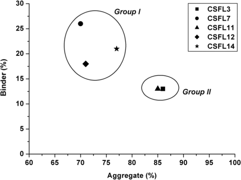
The aggregate/binder ratio establishes two groups of samples (Table 8, Fig. 4). CSFL3 and CSFL11 have a quotient higher than six (group II) and for the other samples the quotient is lower than four (group I).
Colorimetric measurements
Spectral Reflectance Factor of the mortar samples was measured and the CIELAB1976 space coordinates were used for colour specification. The data acquired were relative to the standard observer 10° and D65 illuminant.
Table 9 shows the values of L∗ (lightness), a∗ (green-red axis) and b∗ (blue-yellow axis) obtained for each sample of mortar and cylindrical coordinates C∗ (Chroma) and h (hue angle) derived (Wyszecki and Stiles, 2000).
Table 9
Color data in the CIELAB 1976 space both rectangular L*, a*, b* (respectively Lightness, red-green color component and yellow-blue color component) and cylindrical, C*, h (respectively chroma and hue angle) coordinates with the related uncertainties.
The Fig. 5 shows the numerical brightness values (L∗) associated to hue angle (h) confirming the grouping obtained by XRD analysis. The colour of surface is related to the microscopic structural characteristics and therefore, in cases where it is not possible to extract sufficient material for more accurate characterizations, colorimetry technique could be useful as a tool for mortar classification.
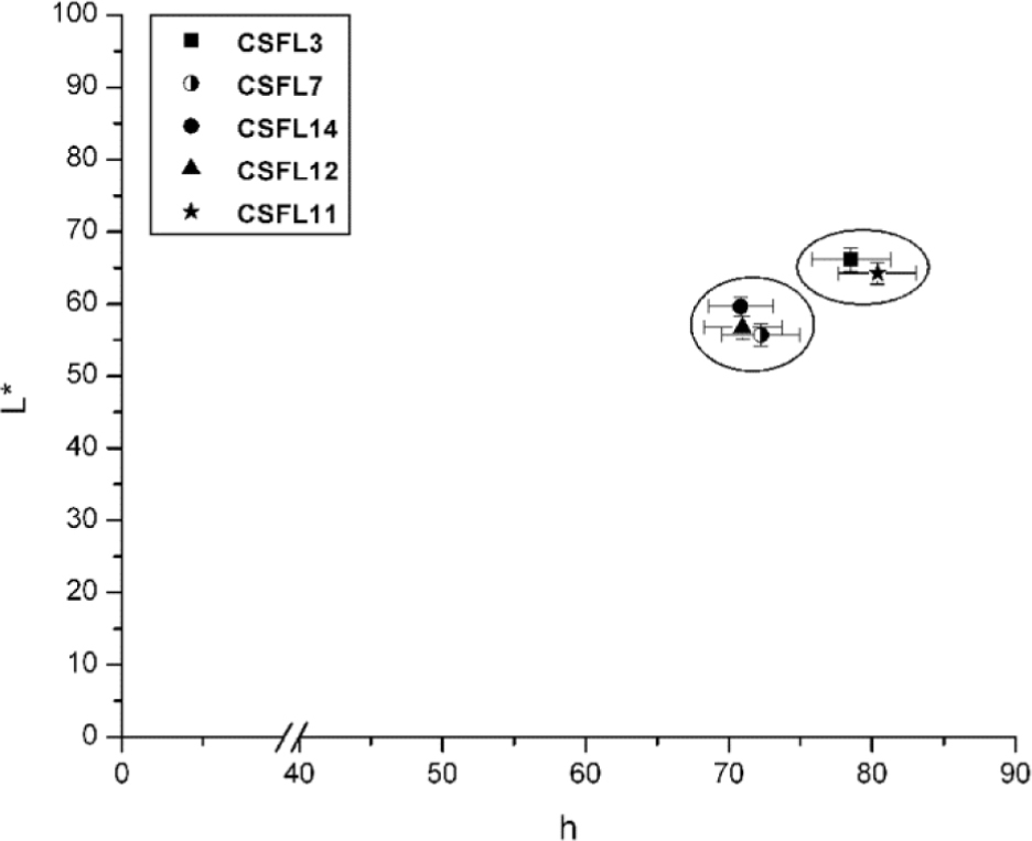
In this specific case this evidence is validated by the good agreement found between colorimetric and XRD results.
. Discussion
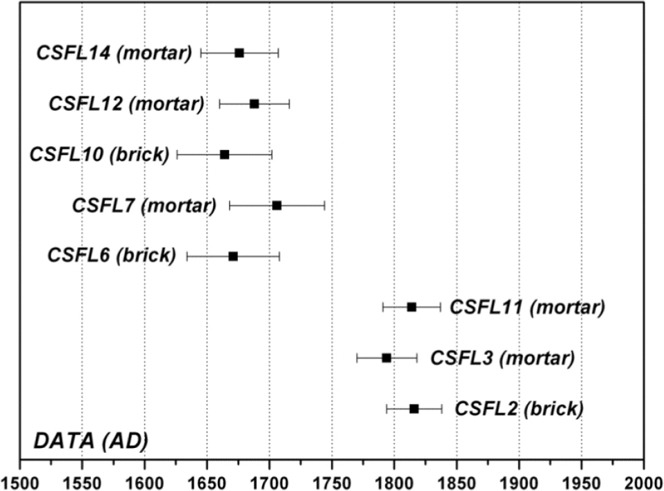
Fig. 6 shows the distribution of dates obtained for the studied mortar and bricks samples. Two sets of dates can be identified: between mid-17th/ mid-18th century; and late 18th/ early 19th century. Good agreement was established between dates obtained for brick-mortar sample pairs CSFL2/CSFL3 and CSFL6/CSFL7, but not for sample pair CSFL10/CSFL11.
Standard statistical analysis and normal distributions obtained for ED measurements of each mortar samples underlined that the used methodology represent an useful approach to obtain indications about the accuracy of the dating results.
The data obtained through mineralogical characterization of mortars identify two different types of materials based on the aggregate/binder ratio. The two groups are confirmed by colorimetric measurements (Figs. 4–5).
Regarding the mineralogical characterization, the methodological approach should have been oriented to the composition and provenance issues if other laboratory tests were available, such as thermal analysis (DTA/TGA) and microscopy (SEM-EDS and/or petrography); chemical analysis; grain size distribution of the aggregates, etc. These complementary methods would make it possible to deeply investigate the composition of the binders and other mortar compounds and to allow a more consistent analysis on materials provenance and composition. Thus, it is only possible to point out the most probable provenance of the aggregates considering only the main characteristics (textural, morphological and mineralogical).
Still, the overall results allowed for a better chronological integration and understanding of stratigraphic data collected, thereby:
– compositional and dating differences between samples CSFL11 and CSFL12 are consistent with stratigraphic observations since the wall corresponding to sample CSFL11 was interpreted as being built over the pre-existing wall correspondent to CSFL12. This is an area of the building which integration in the construction sequence has been harder (Fig. 1), partly due to apparently conflicting stratigraphic observations. This difference in dates between samples CSFL11 and CSFL12, together with the disagreement established between dates obtained for the brick-mortar pair CSFL10/CSFL11, suggests a possible reconstruction phase, resulting in a less clear stratigraphy, already within the industrial occupation, during which brick sample CSFL10 would have been reused;
– the significantly earlier dates obtained for samples CSFL2/CSFL3, allow the integration of the architectural elements from which these were taken within a restructuration of the cells in the late religious occupation of the building, or most likely, already within the industrial occupation;
– the minor interval between samples CSFL12 and CSFL14 dates, although not questioning the proposed construction sequence, suggests the possibility of a close development between construction phases C5 and C3 (Fig. 1);
– this last observation can be also be true when looking at the chronology obtained for pair of samples CSFL6/CSFL7, which also confirms the possibility of its integration in phase C5 (Fig. 1).
. Conclusion
The paper discusses a multidisciplinary approach to the chronological integration of a building with a known complex construction and occupation history.
The results obtained support previous observations regarding the progressive nature of the construction process and the sequence of some building actions, also allowing a first approach to obtain more precise chronological information. It also allowed the integration of some architectural features as later additions to pre-existing construction units.
Furthermore, findings alert to the relevance of using stratigraphic and material analysis information, in order to interpret results from dating analysis, namely difference in date obtained between brick and associated mortars.
We can conclude that the strategic approach is effective for attaining the main purpose of chronological reconstruction of a historical building, namely in the sampling design, selected analytical methods and procedures.