Morphometric and Sub-Watershed Analysis of Taraka Watershed, H.D. Kote Taluk, Mysuru District, Karnataka, India using Remote Sensing and GIS Techniques
Basavaraju
*
 and D. Nagaraju
http://dx.doi.org/10.12944/CWE.16.3.25
Copy the following to cite this article:
Basavaraju B, Nagaraju D. Morphometric and Sub-Watershed Analysis of Taraka Watershed, H.D. Kote Taluk, Mysuru District, Karnataka, India using Remote Sensing and GIS Techniques. Curr World Environ 2021;16(3). DOI:http://dx.doi.org/10.12944/CWE.16.3.25
Copy the following to cite this URL:
Basavaraju B, Nagaraju D. Morphometric and Sub-Watershed Analysis of Taraka Watershed, H.D. Kote Taluk, Mysuru District, Karnataka, India using Remote Sensing and GIS Techniques. Curr World Environ 2021;16(3). Available From: https://bit.ly/31Y52qX
Download article (pdf) Citation Manager Publish History

Introduction
Remote sensing application is wide in all fields especially on aspects of surface covering a large area. Surface feature is very useful for morphometry of particular area of interest in terms of drainage. Remote sensing application using software Arc GIS is very useful analyzing the relationship between runoff, geomorphic and geographic characteristics for morphometry of drainage. The quantitative analysis of watershed gives us an idea about many hydrological aspects. Lithology, slope pedology plays a major role to form watershed. This paper will explain a detail hydrological aspects study area taraka watershed at district Mysore, Karnataka covers 429 km2. Arc GIS maps will be better tool to understand the particular area under study of morphometry on watershed expressed as quantitative analysis description of the drainage pattern in watershed. The establishing of drainage pattern on the behavier of the hyrological system of the watershed area. The quantitative discription and analysis of land forms of drainage basin. The assessment grondwater management groundwater potential zones and physical changes in nature respones over time on drainage system by human impact. A classification of watersheds based on stream oders was first conducted by Horton, which later explained by Strahler(1952)
Material and Method
The GSI topographic map of the 1:50,000 scale map were utilized for delineating the study area. Software using the ArcGIS 9-2.The main concept of the drainage basin are order and length of stream, bifurcation ratios and length of the overland flow(chow,1964;padmini), this is strahler stream classification system.
The basic parmeters are area (A), Stream length (Lu), perimeter(p), watershed length (L), Stream order (Nu) are found out from the watershed map. The diferrent parameters such as Stream length ratio (Rl), Ratio of Bifurcation (Rb), Stream frequency, (Fs), Density of drainage (Dd), Infiltration number (If), Form of factor (Rf), Ratio of Elongation (Re). Circularity ratio (Rc).
Study Area
The Taraka water basin is a part of the river Cauvery basin in the H D KoteTaluk, Mysore District of Karnataka. It is located between 12o00’ to 12o15’ North latitudes and 76o5’ to 76o25’ East longitudes. Taraka watershed, Mysore district, Karnatak state southern part and It comprises of 10 sub-watersheds. The area of study is 429 sq km2. According to Survey of India 57D/4, 57D/8, 58A/1 and 58A/05 are the toposheet number. The study area connected with an all-weather motorable road (Fig.1 and 2). River Cauvery is towards North and H D Kote towards South zone shown in Fig.1. The average rainfall is about 560mm.
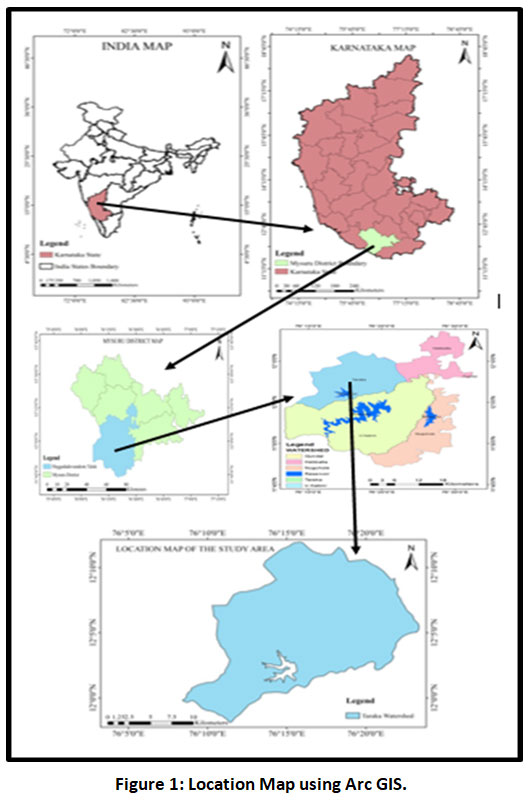 |
Figure 1: Location Map using Arc GIS. Click here to view Figure |
The Lithology of the Area
The taraka watershed is a Proterozoic western block of southern part of Karnataka. Amphibolite Schistose rock of granulite facies of metamorphism which divides the Amphibolite Schist and Granitic Gneissic rocks of Archean age. This area is a typical hard rock terrain (Fig.2 and 3).
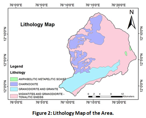 |
Figure 2: Lithology Map of the Area. Click here to view Figure |
Morphometry Analysis
Morphometry was a tool for the measurement and calculative method of analysis to get the quantified values on the surface, shape and dimension of the land. The Taraka watershed is composed of ten sub watershed showing sub-dendritic from dendritic patterns.
Drainage
The procedure by which the water of an area flow off on surface streams or subsurface condition. Natural and artificial methods for effecting discharge of water by surface and subsurface system followed by passages termed as drainage. Geological structure and the natural condition of the soil are the controlling for system flowing movement pattern like vertical and horizontal. Drainage pattern of study area was prepared by toposheets, the 5.8 m spatial resolution and interpretation keys are tone, pattern, texture, and association.
Results and Discussion
Stream Order
The easiest, simplest and widely used numbering is the first tributaries rank of 1 first-order and followed second-order was defined under junction of two first-order streams (Strahler, 1964). In the same 3rd and 4th order will form in Taraka watershed. The stream order was studied 10 sub watersheds of study area. Total 669 streams are present. Out of 10 sub watershed were 5 fifth streams order, 3 were 4th orders of stream, 1 were third and second order streams. First order of stream is present in all 10 sub watershed in an area (Table-1)
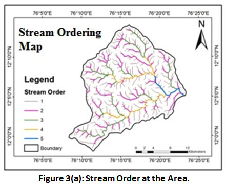 |
Figure 3(a): Stream Order at the Area. Click here to view Figure |
Stream Length
The linear length of river stream is calculated using ARC GIS data analysis techniques. In all watershed first-order which that as streams are lengthier than other which that as the orders of stream increases as the linear length of streams decreased (Horton, 1945). Natural gravity and instable slopes in a place shows this kind of characteristics. The length is high in sub watershed 1 is about 89.59 km and least at sub watershed 6 of 5.861km (Table-2)
Mean Stream Length
Mean length-Lu, of mean channel segment in stream order of u is a dimension property of revealing the size of characteristic the component on a network of drainage and its contributing basin surface (Strahler-1964). To calculate the Total length of channel order of u, total length is divided by the number of segment Nu of that order (Table-3).
Bifurcation Ratio
Bifurcation ratio (Rb) means ratio of stream order to consecutive next order of streams. The 1storder stream doesn’t have tributaries. The 1st and 2nd order streams received by 3rd order streams as tributaries (Schumn, 1956). The 1.06-18.99 value ranges in bifurcation ratio shows the drainage pattern was influenced the geological features and structures. The high value shows stronger geological structures with good topography (Table-4).
Drainage Density
The degree of drainage characterized by development within the basin, purely in qualitative terms such as well-drained and poorly drained are commonly used (Horton, 1945). The controlling factors are length of streams, weathering resistance and rock formations, permeability apart from vegetation and climate. High density drainage is represented in the regions of impermeable and weak and subsurface of hilly regions. The values ranges 0.87-1.29 density of drainage at area was fall under low density (Table-4)
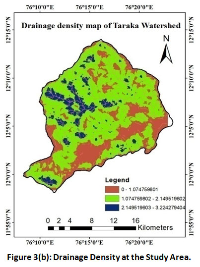 |
Figure 3(b): Drainage Density at the Study Area. Click here to view Figure |
Stream Frequency
It is explained (Horton, 1932) as the stream segments total in number of all total orders per unit area. The values range from 1.31-1.76. The entire 10 sub-watershed indicates fractures controlled channel (Table 3).
Drainage Texture
As per the definition of Smith, 1950 explained in terms of very coarse, coarse and fine texture. The watershed number 3, 5, 6, 8, 9 and 10 were very coarse. Watershed number 2, 4, 7 were coarse texture. Fine texture was absent as per the calculation (Table.4).
Elongation Ratio
It means analysis the basin shape (Schumn, 1956). The values were generally from 0.71 to 1.2. It means geological and climate condition plays a major role. Range from 0.71-1.2 is usually steep slope and high value of relief (Table.4).
Form Factor
The form factor Rf, which are the dimensionless total area of the basin ratio, can be used to indicate the drainage basin of outline shape is quantitative expression of Au of the square of basin length L0,.The area of the ratio square of the streams length.(Horton, 1945). The values ranges from 4.50-20.61 the basin is almost narrowed length basin (Table.4)
Circularity Ratio
As per the definition of Miller (1953), “The ratio0f circularity is expressed as the ratio of the area, The basin area of the circles whose perimeter is equal to the basins of the perimeter” as mentioned in the Table 1. It means stream frequency and stream length. The circularity ratios values Varied from 0.21 –0.73 elongated basin in shape wise.
Length of the Overland Flow
The water flow average length on surface before it became a stream it might be horizontal and drainage divides point finally drains to a same point(Horton, 1945). This is nothing but reciprocal of density of the area drainage. The surface flow water values varied from 0.38 to 0.63. The lithology and physiographic conditions are controlling factor.
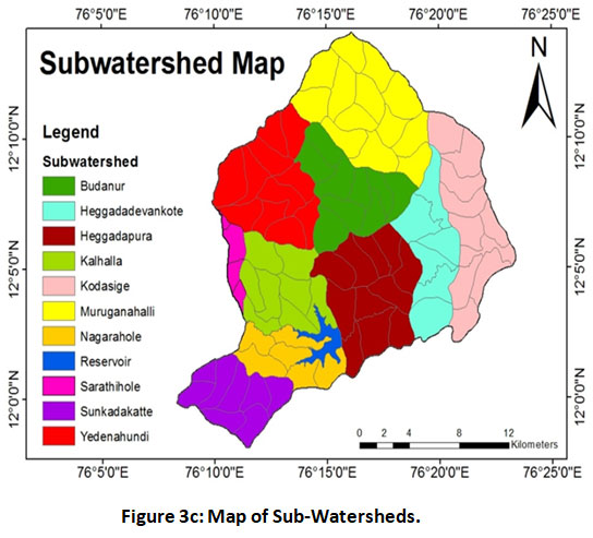 |
Figure 3(c): Map of Sub-Watersheds. Click here to view Figure |
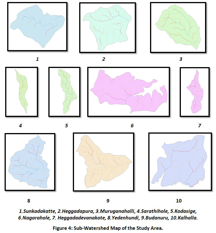 |
Figure 4: Sub-Watershed Map of the Study Area. Click here to view Figure |
Table 1: Parameter of Morphometric and Methodology of Morphometric.
|
Sl.no |
Parameters of Morphometric |
Methodology of Morphometric |
Reference |
|
1 |
Order of Stream (u) |
Order of Hierarchical |
Strahler, (1964) |
|
2 |
Length of Stream (Lu) |
Stream Length |
Horton, (1945) |
|
3 |
Mean Length of Stream (Lsm) |
Lu / Nu = Lsm ; Lu=Mean length of stream order, Nu= Number segments of stream |
Strahler, |
|
4 |
Length of Stream Ratio (Rl) |
Lu/Lu-1= Rl =;Lu =Total length of stream orders (u),Total streams length of next lower order=Lu-1 |
Horton, |
|
5 |
Ratio of Bifurcation (Rb) |
Nu / Nu+1= Rb, Nu=Number of segments in stream present in the order; Segments Number of the higher order= Nu+1. |
Schumn, |
|
6 |
Mean Ratio of Bifurcation (Rbm) |
Average bifurcation ratio of all order = Rbm. |
Strahler, (1964) |
|
7 |
Length of Basin (Lb) |
Straight-line distance between the mouth of a basin and the intersected of point on the water divided on the projection of the line's direction via the main stream's sources. |
Horton, (1932) |
|
8 |
Perimeter (P) |
water divide of Horizontal projection |
Zavoianu, (1978) |
|
9 |
Area of Basin (Ba) |
The complete area of drained by stream systems |
GIS |
|
10 |
Density of Drainage (Dd) |
Lu /Ba= D ;Lu=Total length of Stream of entire area orders (km); |
Horton, (1945) |
|
11 |
Texture of Drainage (Dt) |
Nu/P= Dt ; Total number of stream orders= Nu; P=Perimeter in km. |
Smith, |
|
12 |
Intensity of Drainage ( Di) |
Fs/Dd= Di ; Fs = Frequency of Stream; Density of Drainage.(DD) |
Faniran, |
|
13 |
Frequency of Stream (Fs) |
Nu /Ba= Fs; Nu=Total streams number entire area of all orders |
Horton, (1932) |
|
14 |
Length Flow of Over Land (Lg) |
1/ D×2= Lg; D = Density of Drainage (km/km2) |
Horton, (1945) |
|
15 |
Form Factor (Rf) |
Ba / Lb2 = Rf ;Ba = Basin Area in km2; Lb2 = Square length of basin in km |
Horton, (1945) |
|
16 |
Ratio of Circularity (Rc) |
4×π×Ba/ P2= Rc; Ba = Basin Area ( km2) ;P= Basin Perimeter in km, ℼ = 3.14 |
Miller,(1953) |
|
17 |
Ratio of Elongation (Re) |
√(Ba/π) / Lb= Re; Ba= Basin Area in km2 ; |
Schumn (1956) |
|
18 |
Shape Index (Si) |
Lb2/Ba= Si ; Lb2 = Square length of basin in km; |
Faniran(1968) |
|
19 |
Maintenance of Constant Channel (C) |
C = 1/Dd,, where: Dd = Drainage density |
|
|
20 |
Coefficient of Compactness (Cc) |
0.2841 x (P/Ba 0.5)= Cc ,P = Perimeter in km, Ba = Basin Area in km2 |
Luchisheva, (1950) |
|
21 |
Number of Infiltration (If) |
Fs×Dd= If ; Fs = Frequency of Stream; Dd = Density of Drainage |
Faniran(1968) |
|
22 |
Maximum basin height (Hmax) m |
DEM or GIS analysis |
- |
|
23 |
Basin mouth Height (Hmin) m |
DEM or GIS analysis |
- |
|
24 |
Total Relief of Basin (R) |
R = Hmax - Hmin |
Strahler (1952) |
|
25 |
Ratio of Relief (Rr) |
ð»/ð¿b= ð‘…r ; H = Total basin relief in Kilometer ; ð¿ð‘ =Length of the Basin. |
Schumm (1954) |
|
26 |
Relative Relief Ratio (Rhp) |
R×100/P= Rhp ; R = Maximum relief of the basin |
Melton, (1957) |
|
27 |
Watershed Slope (Sw) |
R/Lb= Sw ; R=Basin Maximum relief, Length of the Basin (ð¿ð‘) |
- |
|
28 |
Aanalysis of Slope (Sa) |
DEM or GIS analysis |
- |
Table 2: Order, Number and Length Streams of Sub-Watersheds.
|
|
|
|
Streams Order |
Streams length (KM) |
||||||||||
|
Sl, no |
Sub watersheds |
Streams order |
I |
II |
III |
IV |
V |
ΣNu |
I |
II |
III |
IV |
V |
ΣLu |
|
1 |
SW -1 |
IV |
62 |
28 |
26 |
6 |
0 |
122 |
45.85 |
23.02 |
16.34 |
4.38 |
0.00 |
89.59 |
|
2 |
SW -2 |
IV |
50 |
19 |
22 |
7 |
0 |
98 |
36.00 |
15.33 |
14.45 |
3.12 |
0.00 |
68.90 |
|
3 |
SW -3 |
V |
37 |
17 |
13 |
0 |
7 |
74 |
29.22 |
15.53 |
8.23 |
0.00 |
5.79 |
58.77 |
|
4 |
SW -4 |
IV |
34 |
10 |
5 |
19 |
0 |
68 |
33.86 |
7.50 |
4.05 |
9.67 |
0.00 |
55.07 |
|
5 |
SW -5 |
V |
27 |
10 |
2 |
11 |
9 |
59 |
28.92 |
6.12 |
1.41 |
6.98 |
5.69 |
49.12 |
|
6 |
SW -6 |
II |
8 |
2 |
0 |
0 |
0 |
10 |
4.26 |
1.60 |
0.00 |
0.00 |
0.00 |
5.86 |
|
7 |
SW -7 |
IV |
44 |
22 |
7 |
16 |
0 |
89 |
36.01 |
16.16 |
4.45 |
9.23 |
0.00 |
65.85 |
|
8 |
SW -8 |
V |
36 |
15 |
12 |
4 |
0 |
67 |
24.78 |
11.34 |
6.69 |
1.74 |
0.00 |
44.55 |
|
9 |
SW -9 |
IV |
19 |
8 |
5 |
1 |
0 |
33 |
12.39 |
5.09 |
2.25 |
0.12 |
0.00 |
19.84 |
|
10 |
SW -10 |
III |
26 |
9 |
14 |
0 |
0 |
49 |
20.95 |
6.09 |
9.57 |
0.00 |
0.00 |
36.61 |
Table 3: Mean and Ratios of Stream Length of Sub-Watersheds.
|
Sl. no |
Sub watersheds |
Mean length of streams (km) |
Length of Stream ratio |
|||||||
|
I |
II |
III |
IV |
V |
II/I |
III/II |
IV/III |
V/IV |
||
|
1 |
SW -1 |
0.73 |
0.82 |
0.62 |
0.73 |
0 |
0.50 |
0.71 |
0.27 |
0.00 |
|
2 |
SW -2 |
0.72 |
0.8 |
0.65 |
0.44 |
0 |
0.43 |
0.94 |
0.22 |
0.00 |
|
3 |
SW -3 |
0.78 |
0.91 |
0.63 |
0 |
0.82 |
0.53 |
0.53 |
0.00 |
0.00 |
|
4 |
SW -4 |
0.99 |
0.75 |
0.81 |
0.5 |
0 |
0.22 |
0.54 |
2.39 |
0.00 |
|
5 |
SW -5 |
1.07 |
0.61 |
0.7 |
0.63 |
0.63 |
0.21 |
0.23 |
4.95 |
0.81 |
|
6 |
SW -6 |
0.53 |
0.8 |
0 |
0 |
0 |
0.37 |
0.00 |
0.00 |
0.00 |
|
7 |
SW -7 |
0.81 |
0.73 |
0.63 |
0.57 |
0 |
0.45 |
0.28 |
2.07 |
0.00 |
|
8 |
SW -8 |
0.68 |
0.75 |
0.55 |
0.43 |
0 |
0.46 |
0.59 |
0.26 |
0.00 |
|
9 |
SW -9 |
0.65 |
0.63 |
0.45 |
0.12 |
0 |
0.41 |
0.44 |
0.05 |
0.00 |
|
10 |
SW -10 |
0.8 |
0.67 |
0.68 |
0 |
0 |
0.29 |
1.57 |
0.00 |
0.00 |
Table 4: Bifurcation Ratios, Density of Drainage, Texture of Drainage, Intensity Drainage and Frequency of Stream of Sub-Watersheds.
|
Sl. no |
Sub-watershed |
Ratio of Bifurcation (Rb) |
Mean ratio of bifurcation (Rbm) |
Stream frequency (Fs) |
Drainage density (Dd) |
Drainage intensity (Di) |
Drainage texture (Dt) |
|||
|
I/II |
II/III |
III/IV |
IV/V |
|||||||
|
1 |
SW -1 |
1.99 |
1.41 |
3.73 |
0.00 |
1.78 |
1.70 |
1.25 |
1.36 |
3.46 |
|
2 |
SW -2 |
2.35 |
1.06 |
4.63 |
0.00 |
2.01 |
1.76 |
1.24 |
1.39 |
2.93 |
|
3 |
SW -3 |
1.88 |
1.89 |
0.00 |
0.00 |
0.94 |
1.44 |
1.14 |
1.26 |
1.82 |
|
4 |
SW -4 |
4.52 |
1.85 |
0.42 |
0.00 |
1.7 |
1.52 |
1.23 |
1.23 |
2.09 |
|
5 |
SW -5 |
4.73 |
4.34 |
0.20 |
1.23 |
2.62 |
1.55 |
1.29 |
1.20 |
1.71 |
|
6 |
SW -6 |
2.67 |
0.00 |
0.00 |
0.00 |
0.67 |
1.41 |
0.82 |
1.71 |
0.58 |
|
7 |
SW -7 |
2.23 |
3.63 |
0.48 |
0.00 |
1.58 |
1.53 |
1.13 |
1.35 |
2.64 |
|
8 |
SW -8 |
2.18 |
1.70 |
3.85 |
0.00 |
1.93 |
1.70 |
1.13 |
1.50 |
1.92 |
|
9 |
SW -9 |
2.43 |
2.26 |
18.99 |
0.00 |
5.92 |
1.31 |
0.79 |
1.65 |
0.86 |
|
10 |
SW -10 |
3.44 |
0.64 |
0.00 |
0.00 |
1.02 |
1.51 |
1.13 |
1.33 |
1.93 |
Table 5: Compactness coefficient, Maintenance of channel Constant, Land flow Length, Shape index.
|
Sl. no. |
Sub watershed |
Compactness coefficient (Cc) |
Maintenance of channel Constant (C) |
Land flow Length (Lg) |
Shape index (Si) |
|
1 |
SW -1 |
0.07 |
0.8 |
0.4 |
0.17 |
|
2 |
SW – 2 |
0.08 |
0.80 |
0.4 |
0.15 |
|
3 |
SW – 3 |
0.11 |
0.87 |
0.43 |
0.24 |
|
4 |
SW – 4 |
0.10 |
0.81 |
0.4 |
0.23 |
|
5 |
SW -5 |
0.13 |
0.77 |
0.38 |
0.26 |
|
6 |
SW -6 |
0.34 |
1.21 |
0.6 |
0.35 |
|
7 |
SW -7 |
0.08 |
0.88 |
0.44 |
0.14 |
|
8 |
SW -8 |
0.12 |
0.88 |
0.44 |
0.19 |
|
9 |
SW -9 |
0.21 |
1.26 |
0.63 |
0.21 |
|
10 |
SW -10 |
0.11 |
0.88 |
0.44 |
0.27 |
Table 6: Basin area, length of the Basin, ratio of Elongation, Perimeter, Form factor, ratio of circularity, Infiltration number and Shape index of the sub watersheds.
|
Sl.no. |
Sub watersheds |
Area of Basin (Ba) Sq. km |
Basin length (Lb) kms |
Perimeter (P) |
Form factor (Rf) |
Elongation ratio (Re) |
Circularity ratio (Rc) |
Infiltration number (If) |
|
1 |
SW -1 |
71.83 |
12.14 |
35.24 |
20.61 |
0.78 |
0.73 |
2.12 |
|
2 |
SW – 2 |
55.78 |
8.7 |
33.44 |
18.91 |
0.96 |
0.63 |
2.18 |
|
3 |
SW – 3 |
51.43 |
12.56 |
40.62 |
14.51 |
0.64 |
0.39 |
1.64 |
|
4 |
SW – 4 |
44.64 |
10.51 |
32.50 |
13.76 |
0.71 |
0.53 |
1.86 |
|
5 |
SW -5 |
37.96 |
9.93 |
34.46 |
12.04 |
0.7 |
0.4 |
1.99 |
|
6 |
SW -6 |
7.11 |
2.50 |
17.12 |
4.50 |
1.2 |
0.30 |
1.15 |
|
7 |
SW -7 |
58.22 |
8.54 |
33.67 |
19.92 |
1 |
0.64 |
1.72 |
|
8 |
SW -8 |
39.38 |
7.64 |
34.78 |
14.24 |
0.92 |
0.4 |
1.92 |
|
9 |
SW -9 |
25.16 |
5.18 |
38.28 |
11.05 |
1.09 |
0.21 |
1.03 |
|
10 |
SW -10 |
32.52 |
9.06 |
25.37 |
10.80 |
0.71 |
0.63 |
1.70 |
Conclusion
The Taraka watershed situated at the south part of Karnataka. River Cauvery is towards North, and H D Kote towards South. The area of study is 429 sq km2. The taraka watershed is composed of ten sub watershed are showing Dendritic to sub-dendritic patterns. Total 669 streams are present out of 10 sub watershed. The length is high in sub watershed number 1 is about 89.59 km and least at sub watershed number 6 is about 5.86km. The bifurcation value ranges from 1.06-18.99. These reading shows the drainage pattern is influenced the geological features and structures. Controlled channel and low drainage density. High relief and almost narrowed channel very coarse 6 watershed and 4 coarse drainage density. The surface flow water depends on the lithology and physiographic conditions are controlling factor.
Acknowledgments
The author would like to thank University of Mysore for granting the Ph.D. research work. The Department of Earth Science, Manasagangothri, Univeristy of Mysore is highly appreciated for allowed the GIS laboratory work. The author is also profoundly grateful to the National Remote Sensing Center (NRSC), Indian Space Research Organization (ISRO), Govt. of India for their guidance during the Satellite data procurement.
Funding Source
This research is funded by university of mysore research fellowship («WÀ 4/28/2018-19 dated 18.06.2019 /267).
Reference
- Agarwal, C.S, Study of Drainage Pattern Through Aerial Data in Naugarh Area of Varanasi DistrictU.P Jour. Indian Soc. Remote Sensing (1998), 26(4): 169-175.
CrossRef - AIS & LUS, Watershed Atlas of India, Department of Agriculture and Co-operation, All India Soil and Land Use Survey(1990), IARI Campus, New Delhi.
- Amit Bera, Bhabani Mukhopadhyay, Debasish Das, "Morphometric Analysis of Adula River Basin in Maharashtra, India using GIS and Remote Sensing techniques", Gatha Cognition(2018).
CrossRef - Binoy Kumar Barman, Gautam Raj Bawri, K. Srinivasa Rao, Sudhir Kumar Singh, Dhruvesh Patel, "Drainage network analysis to understand the morphotectonic significance in upper Tuirial watershed, Aizawl, Mizoram"Elsevier BV(2021).
- Clarke, J.I, Morphometry from Maps. Essays in Geomorphology, Elsevier Publ. Co. (1966), New York, pp. 235-274.
- H. Gupta, B. Hazarika, R. Yenkie, M. Jaunjalkar, S.Verma and D.B. Malpe, Morphometric Analysis of PGW-1 Watershed of Ghatanji Area, Yavatmal District, Maharashtra, Journal of Geosciences Research Vol. 5, No. 2020, Pp-27-34.
- H.S. Kale and S.B. Deshmukh, Morphometric Analysis of WGKD Sub-watershed using Remote Sensing and GIS Techniques, Journal of Geosciences Research Vol. 5, No. 2020, Pp-35-42.
- Horton, R.E, Drainage Basin Characteristics.Trans. Am. Geophys(1932), Union, 13: 350-361.
CrossRef - Horton, R.E, Erosional Development of Streams and their Drainage Basins; Hydrophysical Approach to Quantitative Morphology(1945), Geol. Soc. Am. Bull., 56: 275-370.
CrossRef - J.R. Shrivatra, B.S. Manjare and S.K. Paunikar, Morphometric Analysis Based Prioritization of Sub-Watersheds of WRJ-1 Watershed of Narkhed Taluka, Nagpur District, Maharashtra Using Geospatial Techniques, Journal of Geosciences Research, Vol. 6, No.2, 2021, Pp-242-250.
- Langbein, W.B, Topographic Characteristics of Drainage Basins. U.S. Geol. Surv. Water-Supply Paper(1947), 986(C): 157-159.
- M. Rudraiah, S. Govindaiah, S. Srinivas Vittala. "Morphometry using remote sensing and GIS techniques in the sub-basins of Kagna river basin, Gulburga district, Karnataka, India", Journal of the Indian Society of Remote Sensing(2009).
CrossRef - Miller, V.C, A Quantitative Geomorphic Study of Drainage Basin Characteristics in the Clinch Mountain area, Virginia and Tennessee (1953), Proj. NR389-402, Tech Rep 3, Columbia University, Department of Geology, ONR, New York.
- NRSA, Integrated Mission for Sustainable Development Technical Guidelines, National Remote Sensing Agency (1995), Department of Space, Government of India, Hyderabad.
- P.B. Kamble, J.U. Shinde, M.A. Herlekar, P.B. Gawali, B.N. Umrikar, A.M. Varade and S. Aher, Morphometric Analysis of Ratnagiri Coast, Western Maharashtra, Using Remote Sensing and GIS Techniques, Journal of Geosciences Research, Vol. 4, No. 2 July 2019, Pp-185-195.
- Prafull Singh, Jay Krishna Thakur, U. C. Singh, "Morphometric analysis of Morar River Basin, Madhya Pradesh, India, using remote sensing and GIS techniques", Environmental Earth Sciences. (2012).
CrossRef - Ravi Shankar, Ashok Kumar Singh, Gyan Prakash Satyam, Heidi Daxberger, "Active tectonics influences in the Satluj river basin in and around Rampur, Himachal Himalaya, India", Arabian Journal of Geosciences (2020).
CrossRef - Reddy, P.R.R. and Rangaswamy, C.Y, Groundwater Resources of Pavagada Taluk, Tumkur District. Groundwater Studies No. 240. Department of Mines and Geology (1989), Government of Karnataka, Bangalore.
- S. C. Bhatt, Rubal Singh, M. A. Ansari, S. Bhatt, "Quantitative Morphometric and Morphotectonic Analysis of Pahuj Catchment Basin, Central India", Journal of the Geological Society of India. (2020).
CrossRef - S. P. Rajaveni, K. Brindha, L. Elango, "Geological and geomorphological controls on groundwater occurrence in a hard rock region", Applied Water Science (2015).
CrossRef - S.P. Masurkar, B.S. Manjare and N. Anusha, Morphotectonics of Wan River Sub-basin Using Remote Sensing and GIS Approach, Journal of Geosciences Research, Vol. 4, No. 2 July 2019, Pp -163-172.
- Schumm, S.A, Evolution of Drainage Systems and Slopes in Badlands at Perth Amboy, New Jersey. Geol. Soc. Am. Bull (1956), 67: 597-646.
CrossRef - Srivastava, V.K, Study of Drainage Pattern of Jharia Coalfield (Bihar), India, Through Remote Sensing Technology. J. Indian Soc. Remote Sensing(1997), 25(1): 41-46.
CrossRef - Srivastava, V.K. and Mitra, D, Study of Drainage Pattern of RaniganjCoalfield (Burdwan District) as observed on Landsat-TM/lRS LISS II Imagery. J.Indian Soc. Remote Sensing (1995), 23(4): 225-235.]
CrossRef - Strahler, A.N, Quantitative analysis of watershed geomorphology. Trans. Am. Geophys. Union (1957)., 38:913-920.
CrossRef - Strahler, A.N, Quantitative geomorphology of drainage basins and channel networks. In: V. T. Chow (ed), Handbook of Applied Hydrology. McGrawHill Book Company (1964), New York, section 4-11.
- Y.A. Murkute, S.P. Joshi, S.S. Deshpande and N.G. Oak, Morphometric Study of PG-1 Watershed of Chandrapur District, Maharashtra, Journal of Geosciences Research Vol. 5, No. 2020, Pp-43-51.


