


Abstract
We obtain a simple formula for the stationary measure of the height field evolving according to the Kardar-Parisi-Zhang equation on the interval ![$[0,L]$](https://content.cld.iop.org/journals/0295-5075/137/6/61003/revision2/epl21100337ieqn1.gif) with general Neumann-type boundary conditions and any interval size. This is achieved using the recent results of Corwin and Knizel (arXiv:2103.12253) together with Liouville quantum mechanics. Our formula allows to easily determine the stationary measure in various limits: KPZ fixed point on an interval, half-line KPZ equation, KPZ fixed point on a half-line, as well as the Edwards-Wilkinson equation on an interval.
with general Neumann-type boundary conditions and any interval size. This is achieved using the recent results of Corwin and Knizel (arXiv:2103.12253) together with Liouville quantum mechanics. Our formula allows to easily determine the stationary measure in various limits: KPZ fixed point on an interval, half-line KPZ equation, KPZ fixed point on a half-line, as well as the Edwards-Wilkinson equation on an interval.
Export citation and abstract BibTeX RIS
Introduction
The Kardar-Parisi-Zhang (KPZ) equation [1] describes the stochastic growth of a continuum interface driven by white noise. In one dimension it is at the center of the so-called KPZ class which contains a number of well-studied models sharing the same universal behavior at large scale. For all these models one can define a height field. For example, in particle transport models such as the asymmetric simple exclusion process (ASEP) on a lattice, the local density is a discrete analog to the height gradient [2,3]. In the limit of weak asymmetry, ASEP converges [4], upon rescaling space and time to the KPZ equation. In the large-scale limit, all models in the KPZ class (in particular ASEP and the KPZ equation) are expected to converge to a universal process called the KPZ fixed point [5,6]. Note that the KPZ fixed point is universal with respect to the microscopic dynamics but still depends on the geometry of the space considered (full-line, half-line, circle, segment with boundary conditions).
An important question is the nature of the steady state. While the global height grows linearly in time with nontrivial  fluctuations, the height gradient, or the height differences between any two points, will reach a stationary distribution. It was noticed long ago [1,7,8] that the KPZ equation on the full line admits the Brownian motion (BM) as a stationary measure. It was proved rigorously in [4,9], and in [10] for periodic boundary conditions. For ASEP, stationary measures were studied on the full and half-line [11,12] and exact formulas were obtained on an interval using the matrix product ansatz [13]. The large-scale limit of the stationary measures for ASEP on an interval was studied in [14,15]. The processes obtained there as a limit can be described in terms of textbook stochastic processes such as BMs, excursions and meanders, and they should correspond to stationary measures of the KPZ fixed point on an interval.
For the KPZ equation, while the stationary measures are simply Brownian in the full-line and circle case, the situation is more complicated (not translation invariant, not Gaussian) in the cases of the half-line and the interval. One typically imposes Neumann-type boundary conditions (that is, we fix the derivative of the height field at the boundary) so that stationary measures depend on boundary parameters and involve more complicated stochastic processes (see below). For the KPZ equation on the half-line with Neumann-type boundary condition, it can be shown [16] that a BM with an appropriate drift is stationary (the drift must be proportional to the boundary parameter). This specific stationary measure was studied in [17] for the equivalent directed polymer (DP) problem for which the boundary parameter measures the attractiveness of the wall.
The question of the stationary measure for the KPZ equation on the interval ![$[0,L]$](https://content.cld.iop.org/journals/0295-5075/137/6/61003/revision2/epl21100337ieqn3.gif) has also remained open. In a recent breakthrough, Corwin and Knizel obtained [18] an explicit formula for the Laplace transform (LT) of the stationary height distribution (for L = 1, and for some range of parameters). This LT formula relates the stationary measure to an auxiliary stochastic process called continuous dual Hahn process. This construction corresponds to the KPZ equation limit
1
of formulas with a similar structure obtained in [20] for the stationary measure of ASEP. However, obtaining a characterization of the process allowing to study properties of the stationary measure remains a challenge. This amounts to invert the complicated LT in [18].
has also remained open. In a recent breakthrough, Corwin and Knizel obtained [18] an explicit formula for the Laplace transform (LT) of the stationary height distribution (for L = 1, and for some range of parameters). This LT formula relates the stationary measure to an auxiliary stochastic process called continuous dual Hahn process. This construction corresponds to the KPZ equation limit
1
of formulas with a similar structure obtained in [20] for the stationary measure of ASEP. However, obtaining a characterization of the process allowing to study properties of the stationary measure remains a challenge. This amounts to invert the complicated LT in [18].
In this letter we obtain a simple formula for the stationary measure of the KPZ equation on an interval of any size L, with general Neumann-type boundary conditions. Our result is particularly convenient to study various limits as  . In particular we recover the phase diagram for stationary measures of the KPZ fixed point on an interval, we obtain new crossover regimes near the critical point, and we study the stationary measures of the KPZ equation on a half-line and their large-scale limits. We unveil and exploit a surprising connection to Liouville quantum mechanics (LQM), i.e., the Schrodinger equation in an exponential potential. The LQM, which is the 1D limit of the 2D Liouville field theory, notably allows to study the statistics of exponential functionals of the BM, see [21] for a short review. As such, it appears in several areas of physics such as diffusion in 1D random media [21,22], multifractal eigenfunctions of random Schrodinger and Dirac operators [21,23], diffusion in the hyperbolic plane [24], and more recently, and strikingly, in quantum chaos and its relation to gravity [25,26]. LQM was recently used to obtain multipoint observables for the stationary KPZ equation in a half-space (see the supplementary material in [17]).
Model
The KPZ equation for the height field h(x, t) reads

where  is a standard space-time white noise. We use space-time units so that
  and
and  (see footnote
2
). Here we study the problem on the interval so that (1) holds for 0 < x < L. The solution is defined from the Cole-Hopf mapping
(see footnote
2
). Here we study the problem on the interval so that (1) holds for 0 < x < L. The solution is defined from the Cole-Hopf mapping  , where Z(x, t) equals the partition sum of a continuum DP with endpoint at (x, t) in a random potential
  . It satisfies the stochastic heat equation (SHE)

in the Ito sense, with Robin boundary conditions

and it will be convenient to define boundary parameters  and
and  . Although Z(x, t), t > 0, is not differentiable, the standard way to understand (3) is to impose these conditions on the heat kernel [19], or through a path integral as in [27,28]. For the DP, A > 0 corresponds to a repulsive wall and A < 0 an attractive one, and similarly for B at x = L.
Main result
Our main result is the prediction that the KPZ random height profile in the stationary state, denoted as ![$\left\lbrace H(x) \right\rbrace_{x\in [0,L]}$](https://content.cld.iop.org/journals/0295-5075/137/6/61003/revision2/epl21100337ieqn13.gif) , can be written as the sum of two independent random fields
, can be written as the sum of two independent random fields

where W(x) is a one-sided BM (i.e., with  and W(L) free) and the probability distribution of the process X(x) is given by the path integral measure

with  and X(L) free, and
  a normalization such that
  . For the choice
  ,
,  is thus simply a standard BM. The BM with drift u is also stationary for the half-space KPZ equation [16], and on the segment it arises only when the two boundary conditions are compatible.
In mathematical terms, X is a continuous stochastic process on ![$[0,L]$](https://content.cld.iop.org/journals/0295-5075/137/6/61003/revision2/epl21100337ieqn20.gif) whose measure
whose measure  is absolutely continuous with respect to that of a BM with diffusion coefficient
  , denoted
  , with Radon-Nikodym derivative
  , where

This is a mere reformulation of (5) in a more symmetric form so that it becomes apparent that the process is left invariant after reversing space and exchanging u, v. This reformulation simply means that for any continuous and bounded functional F of the process ![$X=\left\lbrace X(x) \right\rbrace_{x\in [0,L]}$](https://content.cld.iop.org/journals/0295-5075/137/6/61003/revision2/epl21100337ieqn25.gif) ,
,

where in the r.h.s., ![$B=\left\lbrace B(x) \right\rbrace_{x\in [0,L]}$](https://content.cld.iop.org/journals/0295-5075/137/6/61003/revision2/epl21100337ieqn26.gif) is a BM with diffusion coefficient
is a BM with diffusion coefficient  . Surprisingly the measure defined here in (5) as the steady state of the KPZ equation has been already introduced and studied by Hariya and Yor in a different context [29]. We will use some of their results below.
Liouville quantum mechanics
The Liouville Hamiltonian  on the real axis
  is defined as

Its eigenfunctions  , in coordinate basis
  , can be chosen real and indexed by
  with
with

where  and
and  is a modified Bessel function. They form a continuum orthonormal basis with
  with
with  . We will need the matrix elements of the operator

which read

for any  , where
  is a product of four Gamma functions.
Multipoint LT
We now compute, using LQM, the multipoint LT of the distribution of H(x), as defined in (4), (5). For the moment, we restrict ourselves to u, v > 0, and we will discuss the general case later. We consider the increasing sequence of points

Since W is simply a BM independent of X, the following multipoint expectation, with parameters  , takes the form

where  is the following expectation over the process X(x), from (5), with
  :
:
where ![$Z_L[X]:= \int_0^L e^{-2 X(x)}$](https://content.cld.iop.org/journals/0295-5075/137/6/61003/revision2/epl21100337ieqn42.gif) . Now we insert in the integrand the following representation:
. Now we insert in the integrand the following representation:

Performing the change of variable  , and defining the process
  , the RHS of (14), i.e.,
  , takes the form
In the last line we recognize the path integral representation of the imaginary time Green's function of the Liouville Hamiltonian  in (8). From the Feynman-Kac formula
Hence we can rewrite  with
with
Inserting the spectral decomposition

and using the definition (10), the RHS of (16) becomes
Now we use that for w > 0

and  to integrate (18) w.r.t. U0 and
  . We can then substitute the matrix elements
  by their explicit expressions from (11). This leads to
Comparison with the result of Corwin-Knizel
Now, we explain why our formula for the stationary measure in (4) and (5) is equivalent to the LT formula of Corwin-Knizel [18] for L = 1. Again, we assume that u, v > 0 with u < 1 (though [18] provides formulas for the whole range  ). The LT of the stationary height H(x) is expressed in [18] in terms of a Markov process
  with values on
  , called the continuous dual Hahn process (CDHP). The transition probability for
  given
given  , with
  , is given by
and the marginal PDF of  at time s is given by
Then the LT is obtained, for  , as
, as

with (upon some rewriting of formula (1.12) in [18])

and  . It is now a simple exercise to check, using the change of variables
  , that the above formula implies that

Since the prefactor cancels in the ratio, the multipoint LT (13) of our formula (4), (5) written more explicitly in (18), coincides with the result of [18] in the domain u, v > 0 and for L = 1.
We may now extend the result of Corwin and Knizel in two directions. First, we may assume that L is arbitrary, and reproduce the analysis of [18] with points xi as in (12) using the same scalings as in [18] starting from the ASEP model on NL sites and arriving at the same formula (21). This shows why (4), (5) are correct for any L > 0 and not only L = 1 as considered in [18]. Then, we may extend the range of parameters u, v. We expect that the distribution of stationary measures depends analytically on u, v for finite L. However, performing a direct analytic continuation on (21) is intricate and would involve many residues. This is why it is useful to rewrite, through LQM, the results of Corwin and Knizel as in (4), (5), which depends on the parameters in an analytic way for all u, v.
Thus, from now on we will assume that our result for the stationary probability (5), (4) holds for any u, v, and explore the consequences.
Remark: eq. (21) relates the LT of the KPZ height field under the stationary measure to the LT of another Markov process, the CDHP, where the role of time/space parameters and LT parameters are exchanged. The CDHP can be interpreted as living in the Fourier space dual to the real U space of LQM. A similar duality holds for Brownian excursions [30] and can be obtained as a limit of (21) as  , as we shall see in the sequel. Note also that an analog of (21) has been established for ASEP [20], and it would be interesting to study the connection to discrete variants of LQM [31]. It would be also very interesting to know if such dualities extend to other solvable models in the KPZ class.
Limits and consequences
To study the various limits, we define the scaled processes  ,
,  and
and  , with
 ![$\tilde x=x/L \in [0,1]$](https://content.cld.iop.org/journals/0295-5075/137/6/61003/revision2/epl21100337ieqn65.gif) as
as

so that one has

Clearly  is also a standard BM. In order to impose Neumann-type boundary conditions on
  (with slopes
  ,
,  respectively at each boundary) we scale boundary parameters as

The measure for  can then be written, up to a normalization, as
 ![$\mathcal D \widetilde X e^{ - S[\widetilde X] }$](https://content.cld.iop.org/journals/0295-5075/137/6/61003/revision2/epl21100337ieqn71.gif) with the action
with the action
with  and
and  free.
free.
Limit 

In this limit one recovers the Edwards-Wilkinson model. One sees that in (26) we can expand up to linear order in  in the logarithmic terms, and one finds that to leading order in L, i.e., to L0, it becomes a Gaussian action with a parabolic mean profile. One finds (see details in the Supplementary Material Supplementarymaterial.pdf (SM))

where  is a standard BM.
Limit (KPZ fixed point)

Under the scalings considered above,  converges to a probability measure proportional to

with  . Hence it is a BM on
 ![$[0,1]$](https://content.cld.iop.org/journals/0295-5075/137/6/61003/revision2/epl21100337ieqn80.gif) with a nontrivial Radon-Nikodym derivative depending on
with a nontrivial Radon-Nikodym derivative depending on  (equivalently a BM with drift
  with derivative depending only on
  ). The measure can also be rewritten in a more symmetric form as

As detailed in the SM the measure (28) can be studied using a limit of LQM, where the exponential potential is replaced by a hard wall. Accordingly all the above LT formula (13)–(20), are obtained for the rescaled process and parameters by simply replacing  . The field
  should correspond to stationary measures of the KPZ fixed point on the interval
 ![$[0,1]$](https://content.cld.iop.org/journals/0295-5075/137/6/61003/revision2/epl21100337ieqn86.gif) with boundary parameters
with boundary parameters  , and it is natural to predict that they arise as scaling limit of stationary measures of all models in the KPZ class on an interval. This is partially confirmed in some special cases that we study next, where we recover results obtained in [14,15] for the large-scale limit of ASEP stationary measures.
Phase diagram
Now we study the phase diagram in fig. 1, obtained in the L → ∞ limit when u, v are fixed (equivalently when  go to ±∞).
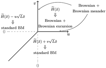
Fig. 1: Phase diagram of the large-scale limit of stationary measures for the KPZ equation on the segment. On the three regions u, v > 0 (maximal current phase), v > u < 0 (low-density phase) and u > v < 0 (high-density phase), we have indicated the nature of the stationary measure in the large-scale limit. For the DP the phases are as follows: for u, v > 0 the DP is delocalized in the bulk, for v < 0, u > v it is bound to x = L, and for u < 0, u < v it is bound to x = 0. Exactly at the phase boundary u = v the DP has probability  to be bound to either side.
Download figure:
Standard imageWhen

In that case the weight in (29) vanishes unless  and
and  , in which case the weight is 1. The second identity taken at
  , together with the first taken at
  implies that
  . Thus, in the limit
  ,
,  , where E is a standard Brownian excursion (i.e., a Brownian bridge conditioned to stay positive), so that

We recover the same process as in the large-scale limit of TASEP [14] or ASEP [15] invariant measures. This shall not be a surprise: TASEP, ASEP and the KPZ equation all converge at large time to the KPZ fixed point [32], so that the process (30) describes the stationary measure of the KPZ fixed point in the so-called maximal current phase for ASEP, that is with repulsive boundary conditions in terms of the DP model.
When or

When  (equivalently
  ) the weight in (29) vanishes unless
  , hence
  is now a Brownian meander (a BM conditioned to stay positive up to time 1). We recover the same stationary process as in the large-scale limit of ASEP stationary measures [15]. Similarly, when
  (equivalently
  ),
),  tends to a Brownian meander, and again, this matches with [15].
When u or v may be negative
By symmetry, we only need to consider the case where v is negative. The measure for X(x) in (5) is a Brownian measure with drift  weighted by
 ![$Z_L[X]^{-(u+v)}$](https://content.cld.iop.org/journals/0295-5075/137/6/61003/revision2/epl21100337ieqn110.gif) , where
, where ![$Z_L[X]=\int_0^L \textrm{d}x e^{-2 X(x)}$](https://content.cld.iop.org/journals/0295-5075/137/6/61003/revision2/epl21100337ieqn111.gif) . We may rewrite (7), up to a renormalisation, as
. We may rewrite (7), up to a renormalisation, as

where  denotes a BM with drift
  and diffusion coefficient
  . It is well known that
 ![$Z_L[B_{-v}]$](https://content.cld.iop.org/journals/0295-5075/137/6/61003/revision2/epl21100337ieqn115.gif) converges as L → ∞ to a finite random variable
converges as L → ∞ to a finite random variable ![$Z_{\infty}[B_{-v}]$](https://content.cld.iop.org/journals/0295-5075/137/6/61003/revision2/epl21100337ieqn116.gif) distributed as an inverse Gamma law with shape parameter
distributed as an inverse Gamma law with shape parameter  [22,33], which becomes asymptotically independent of the rescaled process
  . In order for
 ![$Z_{\infty}[B_{-v}]^{-(u+v)}$](https://content.cld.iop.org/journals/0295-5075/137/6/61003/revision2/epl21100337ieqn119.gif) to have a finite expectation, we need to assume that
to have a finite expectation, we need to assume that  , that is u > v. Thus, we are considering the whole high-density phase in fig. 1. At this point, we find that the resulting measure for
  is simply the standard BM. In the low-density phase where u < 0 and v > u (see fig. 1), we deduce by symmetry that the limiting stationary process is a standard BM with drift
  .
.
Half-line KPZ equation
Consider the KPZ equation (1) in  , with boundary parameter u at x = 0. The stationary measures of the height field can be computed as the L → ∞ limit of the stationary measures defined in (4) and (5) and depending on parameters u, v. It turns out that this limit was studied in [29] (see also the review [34]). We will make considerable use of these results here. The set of stationary measures obtained in the L → ∞ limit always depend on the boundary parameter u, and sometimes depend on the parameter v. When this is the case v can be interpreted as minus the average drift of the process at infinity (see below).
In the low-density phase  , the stationary measure (4) simply converges as L → ∞ to a standard BM with drift u [29] (so that the limit does not depend on v). In the maximal current phase
  , the stationary measures converge [29] to a distribution that we denote
  —the letters
  stand for Hariya-Yor. This is the distribution of the process

where B(1)(x), B(2)(x) are two independent BMs with diffusion coefficient  and
and  is an independent Gamma random variable with shape parameter u. Again, the limit does not depend on v. In the high-density phase
  , the stationary measures converge [29] to a distribution that we denote
  . This is the distribution of the process

where B(1)(x), B(2)(x) are two independent BMs with diffusion coefficient  and
and  is an independent Gamma random variable with shape parameter u –v. In this phase, the limit depends on v, and we remark that the drift at infinity of the process (33) is
  (in the sense that
  when
when  ).
).
We expect that for a large class of initial conditions with drift  at infinity, the height field will converge at large time (modulo a global shift) to one of the stationary measures that we have just described, according to the phase diagram in fig. 2. This prediction is based on an analogous convergence result at large time for ASEP on a half-line proved in [11], though the stationary measures were explicitly described much later [13,35].
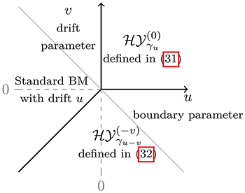
Fig. 2: Phase diagram of stationary measures for the KPZ equation in the half-space  with boundary parameter u. The diagram means that if the initial condition has drift
  at infinity, the height field should converge at large time under mild assumptions to the stationary measure indicated in one of the three regions of the (u, v)-plane. In particular, if
  and the drift at infinity is 0, which includes the flat initial data, the height field will converge to a BM with drift u, as predicted in [17]. Along the antidiagonal line
  , the stationary measure is always a BM with drift u, see the SM.
Download figure:
Standard imageLarge-scale limit
Now that we have described the stationary measures of the KPZ equation on a half-line, it would be interesting to consider their large-scale limit as x goes to infinity. The processes obtained in this limit should be understood as stationary measures of the half-space KPZ fixed point, that is the universal process arising as scaling limit of all half-space models in the KPZ class. In particular, we conjecture that the large-scale limit of half-line ASEP stationary measures [35] does converge to the same limit at large scale. Note that this half-space KPZ fixed point has not been defined rigorously (unlike the full-space situation), but its multipoint distributions for some initial conditions are known [36–37]. The large-scale limit of half-line KPZ equation stationary measures is described in the phase diagram of fig. 3. We will let  and define
  and scale the boundary parameter as
  . In the low-density phase, clearly, the BM with drift u becomes a BM in the variable y with drift
  in the scaling limit. In the maximal current phase
  , the large-scale limit of (32) yields

where  are two independent BMs with diffusion coefficient
  and
and  is an independent exponential random variable with rate parameter
  . Here we have used that
  converges to an exponential distribution with parameter
  . In particular, when
  , we obtain the sum of a BM and a Bessel 3 process [38]
3
, that is a BM conditioned to remain positive on
, we obtain the sum of a BM and a Bessel 3 process [38]
3
, that is a BM conditioned to remain positive on  . In the high-density phase
  , we scale
  and the large-scale limit of (33) yields

where  are two independent BMs with diffusion coefficient
  and
and  is an independent exponential random variable with parameter
  . Again,
  represents the drift at infinity of the process
  . When
  , the process (35) becomes a standard BM with drift
  as this was already the case before taking any limit, although this is not immediately obvious from (35).
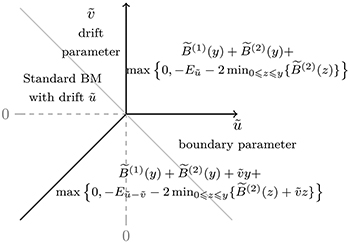
Fig. 3: Large-scale limits of stationary measures of the half-space KPZ equation described in fig. 2.  and
and  denote independent BMs with diffusion coefficient
  .
.  and
and  denote independent exponential random variables with parameters
  and
and  . The parameters
  are rescalings of the parameters u, v in fig. 2 as explained in the letter.
Download figure:
Standard imageDP endpoint
We obtain the endpoint probability for a very long DP as  , where H(x) is given in (4). The statistics of the ratio
  , where G is a standard Gaussian random variable, requires only the PDF P(Y) of
  , which in some special cases takes a simple form (see the SM). For
  one obtains

with  . At the transition point,
  , P(Y) becomes uniform in
 ![$[-L/2,L/2]$](https://content.cld.iop.org/journals/0295-5075/137/6/61003/revision2/epl21100337ieqn180.gif) consistent with the DP being localized near either boundary with probability
consistent with the DP being localized near either boundary with probability  (see the SM for details, and [39] for an earlier work based on ASEP).
Note
While this work was near completion, the preprint [40] appeared. This paper also performs a LT inversion of the result of [18], although [40] describes the process X differently, as a Markov process with explicit transition probabilities. Both descriptions are equivalent: indeed, their formula (1.7) in [40] can also be read from (16) above.
PLD acknowledges support from ANR grant ANR-17-CE30-0027-01 RaMaTraF.
Data availability statement: All data that support the findings of this study are included within the article (and any supplementary files).
Footnotes
- 1
The limit from ASEP to KPZ was previously investigated in [19]. Remark 2.11 therein explains how to rescale ASEP boundary parameters to obtain the boundary conditions for the KPZ equation.
- 2
The units chosen in [18] amount to rescaling our time as
, immaterial in the steady state. - 3
We thank A. Comtet for an exchange on this point.
