


Abstract
Using ratchets, periodic or irregular oscillations can be transformed into steady translational or rotational motions. Here, we consider a model system that operates as a hydrodynamic ratchet. A polymer is placed inside a narrow channel where an oscillating Poiseuille flow is externally created. The ratchet mechanism is implemented by introducing a feedback control for the lateral position of the polymer through which its mobility becomes effectively dependent on the direction of its motion along the channel. We employ the semi-flexible elastic chain modeling for the polymer and use the method of multi-particle collision dynamics to simulate the fluid. We indeed observe directed motion of the polymer and determine the dependence of the propagation velocity on the model parameters.
Export citation and abstract BibTeX RIS
Introduction
Ratchets are devices that can be used to transform oscillations into persistent directed motion. In everyday life, we encounter them in the clocks where mechanical spring-driven oscillations of the balance wheel generate the precise steady rotation of the arrows. In biological cells, many molecular motors are operating as ratchets which convert cyclic conformational changes in the proteins into a persistent motion. As noted by Feynman [1], ratchets can also rectify irregular oscillations (i.e., fluctuations) provided that the system is not at thermal equilibrium. Various stochastic Brownian ratchets with the particles subject to fluctuating potentials or in the presence of non-thermal noises have been subsequently studied (see, e.g., [2–4]). Detailed investigations of polymer Brownian ratchets, where a polymer in a solvent was subject to a flashing periodic potential, have been performed [5,6] and the behavior of such ratchets in confined geometries has been recently discussed [7]. Effects of hydrodynamic interactions on the collective dynamics of particles in flashing channel potentials were also analyzed [8].
In this letter, we explore a different ratchet mechanism which is based on the active control of the polymer mobility (see also [9]). We consider a model system with a polymer placed inside a narrow channel where an alternating flow is externally created. The velocity of the Poiseuille flow is larger in the middle of the channel and falls down at the borders. Hence, the polymer is dragged differently by the flow depending on its position across the channel. The idea is to control this position and make it dependent on the current direction of motion of the polymer along the channel. In our model, the control is implemented by switching on an external transverse force that quickly brings the polymer to the bottom of the channel and thus reduces its mobility when motion in the non-desirable direction is detected. To demonstrate the principal effect, only the case of a periodically oscillating flow will be considered and a two-dimensional system will be chosen. Similar behavior can, however, be expected for randomly alternating flows and three-dimensional systems. The simulations of the flow field are performed by applying the method of multi-particle collision dynamics (MPCD) [10–15]. Previously, this technique has already been used to consider micro-flows inside narrow channels [16–19] and to analyze the dynamics of polymers in such flows [18–20].
As we find, the directed translational motion of the polymer along the channel in an alternating flow can indeed be achieved and thus the considered system is able to operate as a hydrodynamic ratchet. We discuss how the propagation velocity depends on the parameters of the flow and the feedback control.
Formulation of the model
We consider a semi-flexible polymer which is placed inside a narrow channel with an alternating Poiseuille flow and which is subject to control through the application of an additional transverse force G(t) (fig. 1).
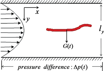
Fig. 1: (Color online) Schematic illustration of the model setup. G(t) is the transverse control force.
Download figure:
Standard imageThe polymer is described as a chain of beads with some bending rigidity. It consists of Nm beads of mass M which are linked by finite-extension nonlinear elastic (FENE) springs with the interaction potential

where kbond is the elastic coupling constant, r is the distance between the adjacent beads and R0 is the maximum distance allowed by the FENE potential. Excluded-volume effects are taken into account through a repulsive Lennard-Jones (LJ) potential

where σ is the diameter of a bead and ε is the potential strength. Bending rigidity of the polymer is taken into account by introducing additional elastic springs which connect next-nearest neighbors [21],

where kbend is the bending rigidity constant, r is the distance of next-nearest neighbors, and the natural length is 4σ.
The fluid is simulated by using the method of multi-particle collision dynamics (MPCD) [13,14,22]. It consists of a set of Ns point-like particles of mass m. Its evolution is modeled by an algorithm which combines streaming and collision steps. In a streaming step, the positions  of all fluid particles are updated according to

where  is the velocity of particle i and τ is the interval between the collisions. In the collision step, the fluid particles are sorted into the cells of a square lattice of lattice constant a and the particle velocities are updated according to a rule adopted from the Anderson thermostat,
here  is the mean velocity of fluid particles in the cell,
  denotes the number of fluid particles in the cell, and
  represents velocities randomly drawn from a Gaussian distribution for each particle, Π is the moment of inertia tensor of the particles in the cell,
  is the relative position of particle i and
  is the center of mass of fluid particles in the cell. To guarantee the Galilean invariance, the grid is shifted randomly before each collision step. No-slip boundary conditions are imposed on the channel walls by the bounce-back rule in combination with virtual wall particles, see [23]. Periodic boundary conditions along the direction of the channel are used.
The interaction of the polymer with the solvent is realized by including its beads in the MPCD collision step [24], so that the center-of-mass velocity is given by
where  is the number of beads within the considered collision cell. The dynamics of the polymer is described by Newton's equations of motions which are integrated using the velocity Verlet algorithm with a time step δt. Between any two MPCD steps, several such time steps are performed to update the positions and velocities of the polymer particles.
The oscillating fluid flow in the channel is produced by applying the same time-dependent pressure force p(t) to each fluid particle,  , where p0 is the pressure amplitude and ω is the oscillation frequency.
The control is exercised by applying the same transverse force G(t) to all polymer beads (fig. 1). In our model, we assume that the control is implemented by an external agent which monitors the motion of the polymer along the channel and switches on and off the force G(t) depending on the current direction of the polymer motion. Specially, we assume that
where X(t) is the position of the center of mass of the polymer at time t and  is the center-of-mass position at a fixed delay Td; the parameter G0 specifies the control intensity. Thus, the force, which tends to bring the polymer to the bottom of the channel, is switched on if the polymer has moved to the right along the channel within time Td; it is absent when the motion has occurred to the left.
Numerical simulations
In the simulations, all distances were measured in units of the bead diameter σ, energy was measured in units of the Lennard-Jones potential strength ε and the time unit was  . For the fluid, the initial velocities of all particles were Gaussian distributed with zero mean and unit variance. The cell size was a = σ, the average number of fluid particles per a cell was
  , and the temperature was
  . The fluid particles and the polymer beads had the same mass
  . The MPCD time step was
  . The time step
  in the integration of the equations of motions for the polymer beads was
  . The control delay time was
  . A polymer with
  beads was placed inside the channel of width
  and length
  . The maximum allowed distance between two adjacent beads was
  , the elastic coupling constant was
  and the bending constant was
  .
.
To test our simulation code, profiles of the mean flow velocity across the channel were determined by applying different permanent pressure differences p0. As seen in fig. 2, the profiles are indeed parabolic and the mean flow velocity vanishes at the channel boundaries, as expected for a Poiseuille flow. Additionally, simulations were performed where the pressure difference was suddenly switched on and the transient process, which established the steady Poiseuille flow, was monitored. The simulations showed that, for the considered channel and for  , the transition time was about
  .
.
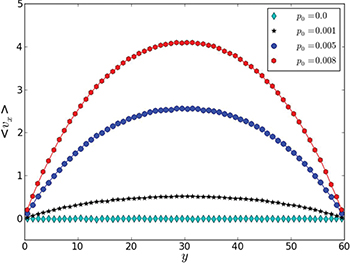
Fig. 2: (Color online) Poiseuille profiles of the mean flow velocity for different constant pressures p0 = 0.0, 0.001, 0.005 and 0.008.
Download figure:
Standard imageResults
Figure 3 shows four snapshots within a single oscillation period of the flow from a typical simulation (the video V1.avi for the entire simulation is available as Supplementary Information). When the polymer moved to the left along the channel, the transverse force G(t) was absent and the polymer chain tended to stay near the middle of the channel where the flow velocity was large(see fig. 3, t = 2460). On the other hand, when the polymer moved in the opposite direction and the transverse force G(t) was switched on, it was tending to bring the polymer closer to the bottom of the channel where the flow velocity was much smaller (see fig. 3, t = 1956). Thus, the ratchet mechanism was implemented. Arrows in fig. 3 are used to indicate the instantaneous local velocity of the hydrodynamic flow. For this purpose, the channel was divided into a square grid of cells of size 6 × 6 and the mean velocities of particles in such cells were chosen to characterize the hydrodynamic flow at the cell location.
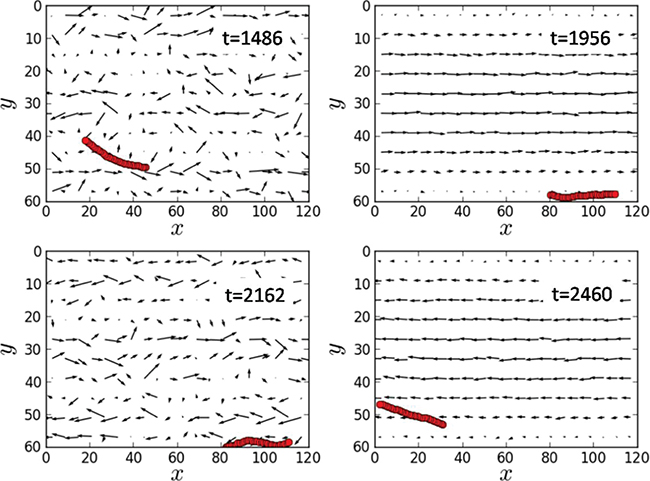
Fig. 3: (Color online) Four snapshots of the polymer in the channel corresponding to different times within one oscillation period of the flow; pressure amplitude  and control force
  . The arrows display the local velocities of the fluid flow. The flow oscillation period is
  . The entire video V1.avi of the simulation is available as Supplementary Information.
Download figure:
Standard imageTo define the location of the polymer inside the channel, the instantaneous position of its center of mass has been used. Figure 4 shows numerically determined probability distributions of the center-of-mass positions across the channel without (fig. 4(a)) and with (fig. 4(b)) the feedback control. In the absence of control, the distribution is symmetric. However, it does not reach its maximum in the channel center, but rather at some neighboring locations. Thus, the polymer tends to avoid the middle of the channel where the flow velocity is maximal; this migration effect was previously discussed in [20,25]. The depletion in the center is less pronounced for the alternating flow (fig. 4(a),  ) as compared with the stationary flow (fig. 4(a),
  ).
).
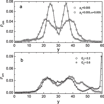
Fig. 4: Distributions of center-of-mass polymer positions across the channel without (a) and with (b) the feedback control. In panel (a), distributions for the constant flow (squares, pressure  ) and for the oscillating flow (pentagons,
  and frequency
  ) at zero control force
  are shown. In panel (b), distributions in the presence of control (diamonds,
  , and stars,
  ) for
) for  and
and  are displayed.
Download figure:
Standard imageWhen the control was switched on, the distribution became asymmetric (fig. 4(b)). It was biased towards the bottom of the channel  since the transverse control force was applied during about each half period. While the asymmetry was relatively small at weak control
  , the distribution developed a peak at the channel bottom for strong control
  , indicating that the polymer was spending much time pressed to the channel boundary by the transverse force. The directed net motion of the polymer in the presence of control is clearly seen in fig. 5(b) and (c); it is absent for
  in fig. 5(a). It can also be noticed that the displacements within each period are much smaller for the strong control force (fig. 5(c)), when the polymer had reached the channel bottom. In addition, we show by (red) dots in fig. 5 the mean positions Xi of the polymer which we obtain by averaging X(t) over the i-th oscillation period of the flow.

Fig. 5: (Color online) Time dependence of the center-of-mass position X(t) along the channel at the feedback intensities (a)  , (b)
, (b)  and (c)
  . Dots indicate the center-of-mass positions averaged over each flow oscillation. The flow oscillation parameters are
  and
and  .
.
Download figure:
Standard imageThe average propagation velocity V of the polymer can be estimated as the average over N oscillation periods,

when calculating this average, we discard the first oscillation period of the flow during which the transients are observed. Averages over 48 oscillation periods have always been performed.
Figure 6 shows the dependence of the computed average center-of-mass velocity of the polymer on the control intensity G0, pressure oscillation amplitude p0, and oscillation frequency ω. As seen in fig. 6(a), the velocity V initially increases with G0, but then starts to decrease. This is explained by the observation that, at large control forces, the polymer is strongly pressed to the channel boundary and does not move much away from it towards the channel center when the force is absent. The optimal ratchet effect is found at  .
.

Fig. 6: Average center-of-mass velocities of the polymer as functions (a) of the feedback intensity G0 for  and
and  , (b) of the oscillation amplitude p0 for
  and
and  , and (c) of the oscillation frequency ω for
  and
and  .
.
Download figure:
Standard imageIn contrast to this, the dependence of the propagation velocity on the oscillation amplitude p0 is monotonous (fig. 6(b)). Note that propagation is absent at  . This means that thermal fluctuations of the flow, which are always present in our simulations, are not sufficient for the considered ratchet effect and the externally induced alternating fluid flows are essential.
There is a strong dependence of the net propagation velocity on the oscillation frequency ω (notice the logarithmic scale for V in fig. 6(c)). The ratchet effect gets progressively weaker as the oscillation frequency is increased. This dependence can be understood by taking into account that, under shorter oscillation periods, the polymer has not enough time to move down to the channel bottom or up towards the middle of the channel when the flow is reversed. Moreover, it can be noted that, when the pressure oscillation period  decreases and becomes closer to the flow transition time
  , the flow has not enough time to fully develop in each oscillation period and its velocity becomes smaller. The largest propagation velocity is found for slowly alternating flows, i.e., when the frequency ω is low.
Discussion and conclusions
Thus, we have demonstrated in our numerical simulations that net propagation of polymers through narrow channels with alternating micro-flows can indeed be achieved by introducing of an appropriate control.
In the considered simple model, we have not specified the nature of the control force and of the control. It was also assumed that the same control forces were acting on all polymer beads. A similar behavior can however be expected if the control force is applied only to a few beads in the polymer chain. In real experiments, the control can be implemented if, for example, tiny metal particles are attached to the polymer and the transverse magnetic field is used to generate the control force. To determine the current position of the polymer along the channel, video microscopy can be employed.
Whereas our simulations were performed assuming periodic alteration of the fluid flow, similar ratchet behavior should also be expected under an irregular alteration of the flow in a channel (such that the net flow is absent on the time average). Note however that natural thermal flow fluctuations are not enough and externally induced alternating flows need to be present. Indeed, as seen in fig. 6(b), directed polymer motion was not observed in the absence of the externally induced periodic flow, i.e. at  . Thermal velocity fluctuations, determined by temperature, are the same anywhere inside the channel. In contrast to externally driven flows, their magnitude does not decrease as the channel boundary is approached. Therefore, the considered ratchet mechanism cannot work in this case.
Generally, the considered ratchet effect should be expected if there is a mechanism which dampens the polymer motion when the polymer moves in the wrong direction and allows its free motion in the desired direction along the channel. In our model, such a mechanism was established through the introduction of a control force, bringing the polymer towards the channel boundary where the flow velocity is low if the motion in the wrong direction was taking place.
One can imagine, however, also other mechanisms which may lead to the same effect. For instance, it can be noted that, in the same Poiseuille flow in a channel, the effective velocity of an object would sensitively depend on its shape. If a polymer is collapsed into a compact globule, it can easily move near the middle of the channel where the flow velocity is high. If, however, the size of the globule is increased and it becomes comparable to the channel width, the motion of the polymer in the same flow would be much slower, because parts of it would be located near the channel boundary where the flow is weak and, additionally, due to the friction against the solid boundaries of the considered channel. This mechanism may also be realized with gels that can swell.
Hence, instead of the control by the application of a transverse force, the suggested ratchet behavior can also be realized by switching on and off the interactions which change the polymer shape. For example, DNA fragments can exhibit phase transitions into a compact globular shape and such transitions can be well controlled [26]. The aim of this letter was to demonstrate the ratchet effect in numerical simulations of a model system. Our conclusions can be tested in specially designed experiments where polymer (e.g., DNA) segments are placed into an oscillating microchannel flow and the control is implemented through an external feedback loop, by optically monitoring polymer positions and manipulating the control force.
An interesting question is whether the considered ratchet effect can also be achieved without an involvement of an external control agent, i.e. by some autonomous "smart" active particles. To do this, such a particle should be able to detect its current direction of motion and, depending on it, change its size or shape. This would require a relatively complex internal machinery which cannot be expected in a simple object, like a polymer molecule. However, such level of complexity can be perhaps reached when protein-coated vesicles are chosen. The proteins can act as receptors that detect the direction and, depending on the receptors'state, phase transitions changing the shape of a vesicle can take place (see also [9]). Investigations of these ratchet systems may represent a promising subject for future work.
Acknowledgments
Financial support from the DFG Research Training Group GRK1558, the DFG Collaborative Research Center SFB 910 (Germany) and from China Scholarship Council is gratefully acknowledged.