The measure of socio-economic status in PISA: a review and some suggested improvements

Abstract

This article reviews the history of the measure of socio-economic status in PISA and identifies theoretical underpinnings of the index of economic, social and cultural status (ESCS). It then highlights multiple changes in the instruments and scaling methods used by PISA over time, and suggests ways of resolving the tensions behind some of these changes and thereby stabilise the measure of ESCS. A stable definition and operational procedure to derive the ESCS index appears essential to compare the ESCS-achievement relationship over time. Some of the suggestions included in this article were already implemented in the 2018 cycle.

Introduction

The index of economic, cultural and social status (ESCS) is probably, just after student achievement scores, the most used variable in reports and in secondary analysis of data from the Programme for International Student Assessment (PISA). Based on student reports to the context questionnaire, it helps address relevant questions about educational opportunity and inequalities in learning outcomes. While well-established and sometimes used as a reference (if not a standard) for the measurement of socio-economic status (SES) in national assessments of school-aged children (INVALSI 2017, p. 70; Cowan et al. 2012), the ESCS index has also been criticised.

Some scholars, in particular, have challenged the validity, reliability or comparability of the current measurement of socio-economic status or of its components in PISA, calling for revisions and extensions of the index (Rutkowski and Rutkowski 2013; Pokropek et al. 2017; Willms and Tramonte 2015).

This article reviews the history and use of ESCS, and formulates recommendations to strengthen its measurement, based on a set of reporting priorities. The significant advances in statistical methodologies since the early 2000s, and more importantly, concerns about the validity of the current measure of socio-economic status in PISA and of the inferences that are made based on it, justify an effort to revisit this variable. The review takes the PISA 2015 database as a starting point: some of the recommendations in this review were shared, in a preliminary version, with the PISA 2018 consortium and were already implemented in the PISA 2018 database.

What is ESCS, and why is it useful?

The PISA index of economic, social and cultural status is closely related to other measures of socio-economic status (SES) that are commonly used in the education literature, in particular within the North American tradition. A report by the “American Psychological Association Task Force on Socioeconomic Status” (APA 2007) described three alternative approaches to define and analyse socio-economic differences in education and in other domains. A first approach (the “materialist” view of SES) summarises the relationship between outcomes (e.g. education) and socio-economic status through the relationship with quantifiable characteristics such as income and wealth. Researchers within this tradition often focus on essential resources and define cut-offs (poverty line, “free-school meal status”) on continuous measures. A second approach (“gradient approaches”) emphasises relative status, and conceives socio-economic status as a unidimensional ranking of individuals in society; this ranking can be informed by multiple dimensions, including, sometimes, subjective ones [such as subjective perceptions of one’s status, measured, for example, through the MacArthur scale (Goodman et al. 2001)]. A third approach focuses on hierarchies of power and privilege and their reproduction (“class models”); researchers following this approach, which is more closely linked to theories of social stratification [e.g. (Weber 1922)], focus on categorical measures, which can be ordered or unordered [for example, “the intellectual elite” vs “the business elite”; (Piketty 2018)].

PISA questionnaire frameworks do not provide an explicit theoretical foundation and definition of economic, social and cultural status (ESCS). The index is operationally defined in the technical reports. For example, the first ESCS variable (constructed for PISA 2000) was simply described as a convenient way to facilitate reporting: “To facilitate the analysis, this chapter combines into a single index the different economic, social and cultural aspects of family background that were examined separately in Chapter 6” (OECD 2001, p. 185).

The ideas and definition that underpin the construction of ESCS must therefore be found in the broader literature, including secondary literature about PISA. According to Doug Willms, who worked on the construction of the first ESCS variable in PISA, ESCS is closely related to the “gradient approach”. Indeed, in reviewing the measure of socio-economic status used in PISA (Willms and Tramonte 2015; Willms 2006), he referred to the definition of socio-economic status by Mueller and Parcel (1981, p. 14):

Socio-economic status is the relative position of a family or individual in a social system in which individuals are ranked according to their access to or control over wealth, power and status.

This definition highlights the relative nature of socio-economic scores as reflecting the hierarchical ranking that characterises modern human societies, while “wealth, power and status” refer to the three components of social stratification highlighted in Weber (1922). In reviewing the broader literature about socio-economic status and achievement, Sirin (2005, p. 418) refers to this same definition as one that can be applied to most studies.

The gradient approach alone however cannot explain PISA’s desire to anchor the measure of socio-economic status on a common scale for all countries and for all years, so as to enable comparisons of “status” across individuals belonging to distinct national societies. The need for such a common scale appears driven by a different definition, which conceptualises socio-economic status not only as one’s position, but as a direct measure of the amount of valued resources and capital that individuals can access and control. This view of “socio-economic status” corresponds to the definition provided by the panel of experts convened at the request of the National Assessment Governing Board to provide recommendations concerning socio-economic status (Cowan et al. 2012):

SES can be defined broadly as one’s access to financial, social, cultural and human capital resources. […]

In sum, the current measure of ESCS and its use in PISA analysis appear inspired by both the materialist view and by gradient approaches. A possible definition of ESCS in PISA therefore is:

ESCS is a measure of students’ access to family resources (financial capital, social capital, cultural capital and human capital) which determine the social position of the student’s family/household.

While commonly used in education research, inferences that rest on a composite measure of socio-economic status—whether conceived as a relative measure of position, or as a unidimensional proxy for different kinds of resources—have also been criticised by prominent scholars (Deaton 2002; O’Connell 2019). Angus Deaton, for example, formulated this critique as follows:

“we have a correlation between socioeconomic status and health and evidence that the correlation is causal, at least in part. [What this implies for policy, however,] depends on what we mean by ‘socioeconomic status’, a term that is convenient as a shorthand for a wide range of possibilities, including income, education, rank, or social class, but that is useless for thinking about policy in the absence of an instrument that acts on them all” (Deaton2002).

A similar critique has also been formulated, within the context of analyses based on PISA data, by Keskpaik and Rocher (2011), who suggest that the individual components of ESCS provide a more useful description of equity in school systems than the unidimensional analysis based on ESCS: a critique that emphasises the multi-dimensional nature of ESCS and is also closely related to “class models”, more typical of the European tradition.

From a measurement perspective, socio-economic status is often conceptualised as a formative latent variable, rather than a reflective latent variable; and the short discussion in this section reflects different views as to whether it should be seen as a causal formative construct (a latent variable that is caused by the observed variables through which it is measured) or simply as a composite formative construct (a convenient, and entirely artificial summary of somewhat unrelated measures) (Bollen and Bauldry 2011).

Our view is that a composite measure of socio-economic status has mainly a practical utility in analysis, avoiding problems that would otherwise arise due to the correlated nature of individual components or due to their interactive effects. In particular, an index such as PISA’s ESCS can be used to build synthetic, high-level descriptive indicators of inequality of opportunity and of outcomes in education, or as a “control” variable to account for the possible confounding effect of pre-existing individual differences on the outcome of interest. While the measure of PISA is inspired by both the gradient and the materialist approach, I suggest to consider ESCS mostly as an artificial composite. In doing so, I make both the individual components and the algebraic operations through which the components are combined part of the definition of ESCS, and redirect questions about the validity, reliability and comparability of the index to its individual components, where such questions are more tractable.

What are the components of socio-economic status?

The definition of ESCS as a composite inspired by the North American tradition of SES measurement suggests constructing ESCS by combining into a single score distinct measures of the financial, social, cultural and human capital resources available to students (and perhaps other resources which are relevant to the family’s position in a particular social hierarchy); this composite score can be thought of as an approximation of individuals’ ranking in a national and global society.

In modern, industrialised societies, it has been common (at least since the first half of the twentieth century) to use formal education credentials, occupation titles converted to a status or prestige scale, and income as the individual components through which socio-economic status is measured. Cowan et al. (2012) note:

Traditionally, a student’s SES has included, as components, parental educational attainment, parental occupational status, and household or family income, with appropriate adjustment for household or family composition. […]

Education, occupation and income are sometimes referred to as the “big three” (Willms and Tramonte 2019); Sirin (2005, p. 418) notes that there is substantial agreement among researchers on the “tripartite nature of SES that incorporates parental income, parental education, and parental occupation as the three main indicators of SES”. Ensminger and Fothergill (2003) note that “education, income and occupation” are the “three most common measures of SES”, but does not recommend combining them into one scale.

The PISA measure of socio-economic status (ESCS) has traditionally been built as a weighted average of three indices: parental educational attainment (in years), parental occupational status on the “International Socio-Economic Index” (ISEI) scale (Ganzeboom 2010; Ganzeboom et al. 1992), and a measure of “household possessions”. Two of the three components that inform the composite score of ESCS—parental years of education and parental occupational status—coincide with those used “traditionally”, according to Cowan et al. (2012). The third component—an index of household possessions, based on the possession or consumption of durable goods—can be thought of as a measure of the household’s income, or more precisely, of its “permanent” component (Friedman 1957).

What reporting goals should inform the measure of socio-economic status in PISA?

Having established the artificial nature of ESCS as a “convenient summary”, its construction should be guided by the validity of the inferences and conclusions that are based on it. A review of existing reports leads to identify the following desirable features for the measure of socio-economic status in PISA:¹

• 1. The PISA data set should include a measure of socio-economic status that supports an analysis of the relationship between student socio-economic status and achievement, through a limited number of key indicators;

• 2. The PISA data set should include a measure of socio-economic status that enables valid comparisons of the relationship between student socio-economic status and achievement across countries and, within countries, over time;

• 3. The PISA data set should include a measure of socio-economic status that enables to classify some students as “vulnerable” or “disadvantaged”, in order to analyse the concentration of such students in particular schools and compare their prevalence, and distribution, over time.

• 4. The PISA data set should include one or more measures of socio-economic status to account for individual differences in endowments and prior achievement, in particular when analysing the relationship between achievement and schooling variables (school tracks, school type, teaching practices, learning practices, opportunity-to-learn variables, …).

• 5. The PISA data set should include a school-level measure of student advantage/disadvantage, which enables to classify some schools as “advantaged” or “disadvantaged” and which can be used in regression analysis (including for the analysis of individual outcomes);

The development of indicators which capture the essential aspects of the relationship between socio-economic status and achievement, and which enable countries to monitor changes in this relationship over time and to compare themselves to other systems, are valued PISA outputs. Indeed, the relationship between students’ socio-economic profile and their performance is an important indicator of the fairness of education systems, i.e. the extent to which good or adverse circumstances (factors that are outside of students’ own control) influence their opportunities to access quality education and reach good learning outcomes; and distributive values such as equality, adequacy and benefitting the less advantaged are at the heart of many education policy decisions (Brighouse et al. 2015).

These needs create a strong rationale for summarising the information about the different components of socio-economic status into a single variable. While it is possible to measure the strength of the relationship between socio-economic status and outcomes in terms of the variation explained by multi-dimensional measures of socio-economic status, this would preclude simple visualisations of this relationship. Multi-dimensional measures also pose challenges for analysing gaps in the average performance of students at different “levels” of socio-economic status (e.g. in different quarters or quintiles), as this would either result in a multiplicity of measures (one per dimension) or in the need to specify distinct discrete profiles or classes to define the levels; in contrast, a single continuous measure allows to simply visualise this relationship and to use simple indicators, such as the gap between the top and bottom quarter of ESCS or the average gap along the continuum (or “slope of the socio-economic gradient”).

Neither of the first two needs mentioned above provides a strong rationale, however, for preferring a particular scale or for assuming a particular distribution for the composite measure of socio-economic status. For example, to avoid choosing a particular scale, a rank- or percentile-measure (which would result in a uniform distribution of socio-economic status) could be used in every country. Non-linear transformations of the composite score, of course, do not result in the same conclusions about the shape of the relationship, and would implicitly re-define the meaning of the “slope”, i.e. of the average gap along the continuum (while a robust, non-parametric definition of the “strength” would be unaffected by such transformations).

Additional reporting needs must be invoked to justify reporting the composite measure of socio-economic status on an interval scale with the same origin in all countries and all cycles. In particular, a common scale presents the advantage of enabling further analyses, such as decomposing the changes in slopes (by distinguishing compositional changes, driven by differences in the underlying distribution of socio-economic status, from shifts in the relationship of socio-economic status and performance). It can also support the development of additional indicators such as the “level” of the socio-economic gradient, i.e. the average outcomes of students at particular points in the distribution of socio-economic status—although due to the artificial nature (and scale) of ESCS, interpretability remains an issue.

The definition of a category of “vulnerable” students, based on some combination of resource indicators, can be a natural by-product of the construction of ESCS or proceed independently. In particular, the definition of levels of vulnerability could explicitly take into account multiple resources and dimensions, without the need to combine them into one measure. At the same time, if the emphasis is on relative disadvantage, a measure that assigns weights to the different dimensions in order to provide a single ranking of students is necessary. In order to enable meaningful comparisons over time or between countries, a composite measure of socio-economic status—or one of its components—should then be reported on an interval scale with the same measurement unit and origin in all countries and over time.

Finally, ESCS is often used as a control variable in regression analyses based on the PISA dataset. The cross-sectional nature of PISA data poses important challenges for the interpretation of analyses that relate resources and processes to outcomes. Measures of family background and socio-economic status can account for possible confounding factors that may create spurious relationships between the outcomes of schooling and the type of school- and out-of-school experiences students have. In such analyses, the direct relationship between outcomes and socio-economic status is of little interest. In some cases, the rationale for including measures of socio-economic status is not to “account” for confounding factors, but simply to increase the precision of estimates; for example, gender can often be expected to be unrelated to family socio-economic status, yet the inclusion of socio-economic status in a regression analysis increases the precision with which gender gaps are estimated.

It is in general preferable to introduce the different components of socio-economic status independently in regression analyses, in order to optimally reduce the variation to be explained and to interpret coefficients on a natural scale, rather than the artificial scale created by the ESCS aggregate. While the different components are related, they are conceptually distinct, and the empirical correlation among different components is unlikely to cause multi-collinearity issues in the large samples that are typical of PISA analysis. However, if interest lies in examining interactive effects (e.g. whether the gender gap is higher among advantaged than among disadvantaged students), focusing on a single measure of socio-economic advantage (which could be a composite measure) greatly facilitates interpretation.

Many policy questions in education are at the school level: how should resources be allocated between schools? When should an additional class be created, or an existing class be closed (and merged with other classes)? Who should decide on the recruitment of new teachers? In analyses related to these questions, it is often interesting to have a school-level measure of advantage and disadvantage. In fact, in many countries, some administrative measures of school advantage exist, because of their use in the funding formula or in staff allocation decisions; for example, “Title I” status in the United States, or the inclusion of the school in a “priority education zone” (ZEP) or “priority education network” (REP) in France. School-level measures that are aggregations of student-level variables, such as the percentage of students eligible for the “National School Lunch Program” (NLSP) in the United States, the percentage of students eligible for “Free School Meals” (FSM) in England, or the percentage of students with low-educated parents, with an immigrant background, or with limited proficiency in the national language, are also often used.

In multi-national studies like PISA, administrative measures are typically not available and not comparable across countries. Instead, one may construct school-level measures of socio-economic (dis)advantage either based on the student sample, or based on specific questions about the entire student body asked to students, teachers, or principals/school administrators. Because of the small within-school samples of students used in PISA, proportions based on the characteristics of sampled students can be affected by significant measurement error, and it may be preferable to use means or medians of continuous measures, rather than proportions of categorical measures. Including more than one measure at the school level can also be problematic, particularly in school-level analyses, due to the small number of schools per country and the high correlation among such measures that can be expected.

In small schools, measures of school advantage that are based on a single grade or cohort of students may give a noisy vision of the school socio-economic profile. The error in the mean estimate is inversely related to the number of students in the sample. In addition, because PISA samples are age-based (as opposed to grade-based), in some cases the PISA sample can give a biased vision of the school profile; such is the case, for example, when the students eligible for PISA are atypical in terms of their grade attainment.²

To overcome this problem, school principals could be asked to provide a measure of socio-economic status that refers to the entire student body or to all students in a particular target grade—for example, the proportion of students that lack the basic necessities or advantages of life, such as adequate housing, nutrition or medical care. Indeed, a similar question was introduced in the PISA 2015 School Questionnaire (SC048) and is used in the “Teaching and Learning International Survey” (TALIS).

Another solution for secondary users of PISA data is to restrict the sample for analyses involving school-level aggregates to schools where “average socio-economic status” is better measured, or to conduct sensitivity analyses. The “Effective Teacher Policies” report, for example, restricted its analysis of school advantage/disadvantage to schools that include the modal level of schooling for 15-year-old students (OECD 2018a, p. 87). The “Equity in Education report” addressed the issue of measurement error (and, to some extent, bias) by restricting the analysis of the relationship between student performance and school socio-economic profile (mean and standard error) to schools in which 10 or more students had a valid ESCS index; sensitivity analyses were conducted (OECD 2018b, p. 137).

How can the current measure of ESCS be improved?

The PISA 2015 Technical Report (OECD 2017, pp. 339–340) describes ESCS as “a composite score derived via principal component analysis (PCA) from the indicators parental education (PARED), highest parental occupation (HISEI), and household possessions (HOMEPOS) including books in the home”:

The next sections will review the instruments and procedures used to derive the composite ESCS index in greater detail. While these instruments have remained similar to when it was first developed, some changes were introduced over time; some of these changes do not appear to reflect methodological advances or new reporting needs. In reviewing each step in the construction of ESCS, the aim is to formulate recommendations for future PISA questionnaires and databases.

For each component, changes in the questionnaire items, and changes in the rules used to derive variables from questionnaire responses will be examined. For the composite measure, changes in the imputation procedure and changes in the weighting scheme will be examined.

Improving the measurement of parents’ or care-takers’ education attainment

The measurement of education attainment in 2015

In 2015, the “parental education” component of ESCS was measured based on questions about father’s and mother’s level of schooling and father’s and mother’s post-secondary educational qualifications.³ These questions were used to identify the highest level of education completed by each parent on a 7-point scale based on the International Standard Classification of Education (ISCED) 1997 (None; ISCED Level 1; ISCED Level 2; ISCED Level 3B or 3C; ISCED Level 3A or 4; ISCED Level 5B; ISCED Level 5A or 6). The highest of the two values was then selected and converted to a years-of-education equivalent (PARED), using conversion tables based on national ISCED mappings, provided by national project managers and documented in an appendix to the technical report.

Issues

The following issues affecting the validity, reliability and comparability across countries and over time of the current measurement of “parental education” can be identified.

Increase in immigrant populations

The substantial increase, in many countries, in the proportion of students with an immigrant background, defies the assumptions behind using national and time-invariant mappings to put educational qualifications (which immigrants may have earned in their home countries) on an SES scale.

Over-reporting of post-secondary qualifications compared to national statistics

At the country level, the proportion of students who report their mothers (fathers) to have tertiary education credentials correlates highly with the proportion of 35–54 year-old women (men) who have such credentials, at least for countries covered by the OECD Education at a Glance database. The linear correlation coefficient is 0.86 for mothers/women, and 0.78 for fathers/men. In general, the rate of tertiary qualifications reported for fathers is higher than the corresponding rate among 35–44-year-old men (and similarly for mothers), suggesting that students over-report tertiary degrees. The extent to which this occurs may vary across countries: Poland and Greece, for example, have similar rates of tertiary attainment among men (below 30%); but only about 20% of students report tertiary degrees for their fathers in Poland,⁴ compared to over 40% in Greece. On the other hand, in Russia, more than 80% of students report their fathers to have a tertiary qualification, while labour-force surveys indicate that only about 45% of men to have such qualifications (Fig. 1).

Fig. 1

(Source: OECD, PISA 2015 Database; Education at a Glance Database (https://stats.oecd.org/OECDStat_Metadata/ShowMetadata.ashx?Dataset=EAG_NEAC))

Tertiary attainment of fathers (PISA) and of 35–44 year-old men (EAG). Pearson’s linear correlation coefficient between the two series is 0.78 (N = 41)

Inconsistency between “level of schooling” and “post-secondary qualifications”

The PISA 2015 measure was based on distinct answer formats for qualifications up to upper-secondary level (ISCED Level 3) and for post-secondary qualifications. By virtue of the hierarchical nature of the ISCED classification, in order to have an ISCED Level 4 degree or higher it is necessary, in theory, to have earned an ISCED Level 3 qualification.⁵ However, a significant number of students report a level lower than ISCED Level 3 as their parents’ highest level of schooling, and at the same time report their parents as having post-secondary qualifications.

Missing answers

The percentage of students with missing reports on both their father’s and mother’s education—and thus for whom no “parental education” component could be computed—is relatively low, but varies considerably across countries and years. The median missing rate across countries for PARED was 1.9% in 2015 (inter-decile range: 0.6–4.5%). The highest missing rate was observed in Germany (17.5%),⁶ the lowest missing rate in Romania (0.04%). The percentage of missing answers fluctuated over time with no clear trend, and no particular change related, for example, to the introduction of computer-based questionnaires in 2015 (Fig. 2).

Fig. 2

(Source: PISA 2003–2015 database)

Percentage of respondents with missing parental education component. The figure represents the median, interquartile range (shaded area) and adjacent values for country-level missing rates in PARED. Adjacent values are defined as the most extreme missing rates within 1.5 times the interquartile range from the nearest quartile. The following countries have missing rates that exceed the upper adjacent value: 2003: Canada (10.9), Germany (11.0), Luxembourg (13.1), New Zealand (11.9); 2006: Germany (6.2), United Kingdom (8.7), Israel (7.2), Luxembourg (6.8), New Zealand (7.9); 2009: Germany (13.0), United Kingdom (8.0), New Zealand (9.3), Panama (16.7); 2012: Germany (21.5), United Kingdom (7.6), Luxembourg (6.8), New Zealand (8.9); 2015: Brazil (6.6), Germany (17.5), United Kingdom (9.3), New Zealand (8.9)

Misreporting

Researchers have questioned whether students provide valid responses regarding their parents’ education. Studies that were able to compare reports by multiple raters have found that students’ reports of parental education have relatively low correlations with parents’ self reports, lower than, for example, correlations among reports of parents’ occupations; in addition, there appears to be considerable variability across countries in inter-rater agreement (Willms and Tramonte 2019; Lien et al. 2001; Looker 1989; Jerrim and Micklewright 2014; Schulz 2005).

Changes over time in questionnaire instruments

The international versions of the parental education questions used different wording and response formats in PISA 2000, 2003, 2006 and 2009, and have since not changed until 2018 (Box 1).

However, more subtle changes have been introduced all along in national questionnaires, in harmonisation rules to map back national adaptations to international response options, and in rules to derive the year-of-education equivalence:

• The mapping of ISCED levels to years of schooling changed a first time in 2006, and was subsequently revised in every cycle in consultation with countries.

• Changes in national adaptations of the international questions—e.g. to distinguish a greater number of tertiary qualifications (bachelor, masters, …)—and/or to the mapping of national response options into international variables (“harmonisation”) are poorly documented, but may affect the comparability of data over time.⁷

Alternative measures

Some issues related to the measurement of parental education are difficult to solve: for example, the misreporting of parental education by students. Other issues may be addressed more simply in revised procedures or instruments, such as:

• Considering students’ answers about post-secondary qualifications only for those students who reported their parents’ highest level of schooling to be at least (lower) secondary education. This has the potential to reduce mis-reporting and the over-reporting of tertiary qualifications, in particular in developing countries where universal primary education was not yet the rule in the parents’ generation. In future questionnaires, this filter rule could be automatically applied at the time of data collection.

• Using a single, international conversion to convert major ISCED levels into their (approximate) years-of-education equivalent. In order to minimise the differences with established patterns, this international conversion could be initially determined by using the modal years of education across countries for each ISCED level. This would eliminate a source of mistakes in the calculation of ESCS and limit arbitrary differences between countries with similar educational structures. The comparability of the parental education component of socio-economic status across countries and over time would therefore rely directly on the comparability of the education levels, before their conversion on an SES scale.

Table 4 (Appendix) uses PISA 2015 data to explore the impact of these suggested changes on the measure of parental years of education in PISA, and on the relationship with performance.

Results included in Table 4 (Appendix) suggest that the introduction of a filter on secondary education and of a common conversion from ISCED levels to years of education would only minimally affect within-country analyses, and has the potential to improve the cross-country comparability of PARED and its use a component of an international measure of socio-economic status. The alternative that incorporates both changes (PARED2) in particular has marginally higher concurrent and criterion validity, as indicated by correlations with country-level measures based on labour-force surveys, with other ESCS components, and with science performance. The correlation with country-level measures based on labour-force surveys measures increases only minimally, across all countries, but a larger increase is observed for lower-income countries (where over-reporting may be more of an issue). The correlation with the “household possessions” component of ESCS (variable HOMEPOS) was investigated in particular on the share of students with values in the top and bottom international quintile of these measures. Indeed, one use of ESCS as an internationally comparable scale is to generate international categories (typically “deciles” or “quintiles”) of resources; and the analysis typically focuses on the extremes (bottom decile, top decile, etc.). Because parental education (PARED) is the most discrete component of ESCS, the actual values used to convert the top and bottom education category onto the ESCS scale loom large on the percentage of students who are classified in the top and bottom quintiles of ESCS. In particular, in 2015, using the national conversion, countries such as Australia, Israel, France and New Zealand (which have relatively small values, for the PARED conversion of tertiary education) ended up having fewer students than one would expect in the top quintile. An international conversion of education levels to the SES scale would result in international rankings of students on the scale that no longer depend on the values chosen to convert tertiary education into years of education, but directly on the qualifications level distinguished in questionnaires. For the purpose of trend analyses, both suggested changes—using a filter on post-secondary education qualifications and a conversion from ISCED levels to years of education that is common to all countries—could be applied retrospectively to past datasets. Trend comparability of the “education” component of socio-economic status would rely directly on the comparability (over time) of major levels of education distinguished in questionnaires; where this comparability can no longer be guaranteed for all education levels distinguished in questionnaires, because of changes in education structures, it may be necessary to merge questionnaire levels into broader categories that remain comparable.

Parents’ occupational status

The measurement of occupational status in 2015

The “parental occupation” component of ESCS is measured based on open-ended questions about father’s and mother’s job title/occupation (questions ST014Q01TA and ST014Q02TA in PISA 2015). Countries are then required to use the information provided by students to assign a code based on the International Standard Classification of Occupation (ISCO) to each student. This international classification developed by the International Labour Organisation (ILO) distinguishes over 400 occupations (4-digit codes, e.g. “carpenters”, “stonemasons”, “roofers”, “plasterers”), grouped into 28 groups (defined by the first two digits of their codes, e.g. “Building and related trades workers, excluding electricians”) and 10 major groups (first digit, e.g. “craft and related trades workers”). PISA has expanded the list of ISCO codes with special codes for unemployed and inactive parents (9701 “Doing housework, bringing up children”, 9702 “Learning, studying”, 9703 “Retired, pensioner, on unemployment benefits”). The ISCO codes provided by countries (which form a nominal scale) are then converted into an ordinal or interval scale using prestige rankings or income rankings based on international studies; PISA refers to the “International Socio-Economic Index of occupational status” (ISEI) developed by Ganzeboom (2010). The highest value for either parent is used in the ESCS composite (HISEI).

Similar to what is proposed above for the education component of socio-economic status, the occupation component already relies on a common mapping, across all countries, of detailed occupational categories on an SES scale. The comparability of the occupation component of socio-economic status across countries and over time therefore relies on the comparability of the occupational codes.

Issues

Accuracy of coding

There are no standards about the quality of coding procedures. Some countries do not code occupations to the four-digit level: until 2009, Japan coded occupations only at the 2-digit level; in 2015, the United Kingdom coded occupations only at the 3-digit level.

Validity of the ISEI conversion across time and countries

The prestige, skill level and income of certain occupations can vary significantly across countries and levels of development (to take just one example, “cattle farmer” can correspond to very different income and skill levels, depending on the national context); but Ganzeboom’s work (Ganzeboom et al. 1992; Ganzeboom 2010) is based on a more restricted set of countries than the set of countries participating in PISA (the most recent conversion of occupational codes to ISEI codes is based on 42 countries or subnational entities that participated in the International Social Survey Programme between 2002 and 2007). Furthermore, the relative prestige and income of certain occupations and the educational requirements to access certain occupations is also subject to change over time (e.g. “teacher”), creating tensions for the conversion of ISCO codes to an ordinal or interval scale.

Missing data

The percentage of students with missing reports on father’s and mother’s occupation is relatively high, and varies significantly across countries. The median missing rate across countries for mother’s occupation (OCOD1) is 12.8% in 2015 (inter-decile range: 6.8–23.8%). The highest missing rate is observed in Algeria (74.8%), the lowest missing rate in Viet Nam (2.0%). The median missing rate across countries for father’s occupation (OCOD2) is 16.6% in 2015 (inter-decile range: 24.5–8.7%). The highest missing rate is observed in Thailand (30.3%), the lowest missing rate in Viet Nam (5.7%). While single-parent households may explain the high levels of missingness to some extent, some scholars attribute high rates of missing data to the open-ended nature of the question (Willms and Tramonte 2015). Figure 3 shows that the median rate of missingness has increased over time, and in particular after 2009. The high level of missingness in low-achieving countries suggests that the response burden for this question may be too high for children with low literacy levels.

Fig. 3

(Source: PISA 2000–2015 database)

Percentage of respondents with missing ISCO codes for parental occupation. Share of missing values for fathers’ (left) and mothers’ (right) occupation codes. The figure represents the median, interquartile range (shaded area) and adjacent values for country-level missing rates in OCOD2 (Father ISCO code) and OCOD1 (Mother ISCO code). Adjacent values are defined as the most extreme missing rates within 1.5 times the interquartile range from the nearest quartile. The following countries have missing rates that exceed the upper adjacent value: Fathers: 2000: Israel (31.1), Japan (65.0), United States (28.3); 2003: Japan (25.4); 2006: Israel (21.7), Japan (22.0), Qatar (44.8); 2009: Georgia (30.3), Panama (25.3), Himachal Pradesh (India) (32.8), Tamil Nadu (India) (26.3); 2012: Albania (31.7), Austria (100), Japan (26.8); 2015: none. Mothers: 2000: Brasil (26.7), Israel (25.5), Japan (66.5), United States (23.1); 2003: Canada (16.4), Germany (16.7), Japan (21.3), Netherlands (15.8), New Zealand (17.8); 2006: Israel (16.5), Japan (16.3), Qatar (31.4); 2009: Canada (16.8), Germany (16.7), Japan (16.2), QTN (24.8); 2012: Albania (27.4), Austria (100), Germany (22.3); 2015: Algeria (74.8), United Kingdom (28.3), Chinese Taipei (37.0), Thailand (29.1), Tunisia (66.2)

In addition, until 2015, no score on the ISEI scale was assigned for the three codes that PISA added to the list of ISCO codes (“Doing housework, bringing up children”, “Learning, studying”, “Retired, pensioner, on unemployment benefits”). As a result, even after combining father’s and mother’s reports in a HISEI value (and thus limiting the impact of single-parent households), missing rates for this component of ESCS remain high. The median missing rate across countries for HISEI is 9.3% in 2015 (inter-decile range: 4.7–17.7%). The highest missing rate is observed in Algeria (24.0%), the lowest missing rate in Viet Nam (4.7%) (Fig. 4).

Fig. 4

(Source: PISA 2000–2015 database)

Percentage of respondents with missing parental occupation component of ESCS. The figure represents the median, interquartile range (shaded area) and adjacent values for HISEI. Adjacent values are defined as the most extreme missing rates within 1.5 times the interquartile range from the nearest quartile. The following countries have missing rates that exceed the upper adjacent value: 2000: Israel (26.0), Japan (62.5), United States (14.6); 2003: New Zealand (14.1); 2006: Azerbaidjan (17.0), Israel (16.1), Jordan (20.7), Qatar (41.2); 2009: Georgia (22.4), Himachal Pradesh (India) (32.6), Panama (17.0), Qatar (19.4), Tamil Nadu (India) (23.4); 2012: Germany (19.5), Jordan (21.8), Montenegro (16.2), Qatar (18.3), United Arab Emirates (15.0). 2015: Algeria (23.4), Thailand (22.8)

Cost

Coding open-ended questions is costly and requires relatively specialised knowledge that national PISA centres do not necessarily have in house.

Alternative measures

Two possible changes to PISA procedures and instruments can address the main issues identified about the parental occupation component of ESCS.

• Assign an (approximate) ISEI code to “non-occupations” identified by the pseudo-ISCO codes 9701, 9702 and 9703 (“Doing housework, bringing up children”, “Learning, studying”, “Retired, pensioner, on unemployment benefits”). A possibility is to use the lowest ISEI code for these occupations (11); this would limit the impact of this change for households where only one of the parents has such a code. Following a similar logic, but to avoid extreme values, I suggest using 17 as the ISEI value for these occupations, as this corresponds to the ISEI value used in PISA for occupations generically classified as “elementary occupations” (ISCO08 equal to “9000”). The extension of the ISEI scale to account for the special ISCO codes used in PISA can eliminate one source of cross-country differences in missing rates and thereby improve cross-country comparability.

• Reduce the coding scheme to 1-digit or 2-digit codes only or use a closed response format to collect information about occupations. The impact of using only 1-digit or 2-digit coding can be explored by recoding existing data to this level of precision only. In contrast, the impact on the validity and comparability of the data collected from closed response questions about occupations can only be investigated based on field-trial data in which both question formats are administered. While the close response format may significantly reduce missingness and costs, it may also have a higher reading load (since all response categories need to be read) and induce socially desirable answers (e.g. due to order effects) to a greater extent than a text-entry field. Reducing the coding scheme to one or two digits would significantly reduce the cost of ISCO coding. It may also contribute to greater cross-country comparability of occupational codes as a result of higher, and more consistent coder reliability. In the absence of information about the current level of coder reliability, however, these gains remain speculative.

Table 5 (in Appendix) uses PISA 2015 data to explore the impact of some of the suggested changes on the parental occupation component of socio-economic status, and on its relationship with performance.

Results indicate that the inclusion of pseudo-ISEI values for the additional occupation codes created by PISA (housewife, etc.) not only reduces missingness for this component, but also results in a higher correlation with science achievement (Appendix, Table 5). By reducing the share of students for whom this component is missing, the inclusion of such pseudo-ISEI values can change the country-level average HISEI (and as a consequence, average ESCS) significantly in some cases, as shown by Jordan, whose mean value decreases by about one fourth of a standard deviation.

Results also suggests that analyses based on the parental occupation component of socio-economic status are relatively robust to changes in the coding scheme that would significantly reduce the data-collection costs for countries. In particular, the use of a more limited number of codes—either 34 two-digit codes or 10 one-digit codes—would have only a limited impact on country rankings and on the estimated correlations with achievement (Appendix, Table 5).

Household possessions

The measurement of household possessions in 2015

In 2015, the “household possessions” component of socio-economic status was based on 25 items in questions ST011 (16 dichotomous items, including 3 chosen by each country), ST012 (8 polytomous items, with a four-point scale) and ST013 (one polytomous item, with a 6-point scale) (see Table 1).

Table 1 International household possession items across survey cycles.

A one-dimensional generalised partial credit model was fitted to the data, with some items receiving country-specific item parameters. This was the case for the three national items in ST011, but also for the two indicators about the possession of “classic literature” and “books of poetry”, for which the meaning and the national examples included in the item stem may vary significantly across countries. Items that showed strong evidence of misfit for particular countries were also assigned national items; this was the case for the indicator on “educational software” in Japan.

Issues

The following issues affecting the validity, reliability and comparability across countries and over time of the current measurement of household possessions can be identified.

Validity of household possessions in cross-country comparisons

A measure of income or consumption for cross-country comparison should be expected to correlate highly with other measures of national income or household income. The country means of the PISA 2015 measure of household possession have a moderate positive correlation (0.65) with per-capita gross national income measures. The correlation is even higher if small countries with large natural resource revenues or financial sectors are excluded, or if income is expressed in a logarithmic scale (Fig. 5).

Fig. 5

(Source: PISA 2015 Database and https://data.worldbank.org)

Correlation of average HOMEPOS (PISA) and GNI per capita (World Bank). Pearson’s linear correlation coefficient between the two series is equal to 0.65 (0.80 when GNI per capita is measured on a logarithmic scale)

Similarly, the percentage of 15-year-old students with a low level on the international household possession scale (values of HOMEPOS below − 1.77) correlates strongly (r = 0.85) with the percentage of the general population living below the World Bank upper middle-income International Poverty Line, set at USD 5.50 (PPP) (Fig. 6).

Fig. 6

(Source: PISA 2015 database and https://data.worldbank.org)

Students with low household possessions and international poverty rates. The smaller, shaded chart shows an enlargement of the shaded area in the larger chart. Pearson’s linear correlation coefficient between the two series is 0.85. Values for Australia, Austria, Belgium, Canada, Cyprus, the Czech Republic, Germany, Denmark, Finland, France, Ireland, Iceland, Luxembourg, Malta, the Netherlands, Norway, Slovenia, Sweden, Switzerland and the United Kingdom, all countries with a poverty headcount ratio at or below 1%, are also shown but not labelled in the charts

Missing answers

The percentage of students with missing reports about their household possessions is relatively low, compared to other components of ESCS. The use of a proxy of family income instead of direct questions about this therefore seems successful at overcoming problems associated with missing answers. Nevertheless, there has been an increase in the rate of missing answers in 2012 and 2015, compared to previous surveys, and driven in particular by higher missing rates in Germany (Fig. 7).⁸

Fig. 7

(Source: PISA 2000–2015 database)

Percentage of respondents with missing household possessions component. The figure represents the median, interquartile range (shaded area) and adjacent values for country-level missing rates in the household possession index (HOMEPOS). Adjacent values are defined as the most extreme missing rates within 1.5 times the interquartile range from the nearest quartile. The following countries have missing rates that exceed the upper adjacent value: 2003: Brasil (2.11), Canada (9.78), Czech Republic (4.14), Germany (5.67), United Kingdom (3.72), Netherlands (3.16); 2006: Bulgaria (2.06), Canada (3.53), Chile (2.05), Germany (3.15), Israel (4.03), Norway (1.98), Qatar (4.47); 2009: Brasil (5.68), Germany (7.04), Panama (6.43); 2012: Albania (6.90), Germany (15.13), Iceland (2.73), Israel (2.86), Qatar (3.24); 2015: Brazil (5.22), Germany (12.64), Russia (4.07), Tunisia (4.17)

Changes in measurement instruments

There have been numerous changes over the years in the instruments used to measure household possessions.

The most visible change is the change in the set of international items in the household possession scale and in the order of items within each question (Table 1). The position of the questions within the questionnaire (at the beginning or at the end) has also changed over cycles.

A second type of change is the change in the answer categories for “Books at home”, which were changed in PISA 2003 to better match those used in other educational studies like TIMSS and PIRLS (Table 2).

Table 2 “Books at home” across survey cycles.

Table 3 International ESCS component weights based on PCA

Table 4 Alternative measures of the “parental education” component of socio-economic status

Table 5 Alternative measures of the “parental occupation” component of socio-economic status.

Less visible changes have also happened over the years. In particular:

• In 2003, the second set of questions about household possessions [Question 18, items (a) to (e)], asking students to count the “number of… at home”, could not be included in the computation of ESCS since they were deleted from the student data file (OECD 2005a, p. 246). The suppression of student responses was necessary because preliminary analyses revealed that students were confused by the data-entry codes that were printed next to the answer boxes, and which contradicted the answer categories for students provided above the boxes. It must be noted that these small numbers were re-introduced in 2015 for paper-based instruments (in use in a small minority of countries), but no similar action was taken (Fig. 8). In 2018, two-digit data-entry codes (“01”, “02”, “03”, “04”) were used in countries that continued to administer paper-based instruments.

  Fig. 8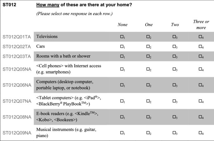

  

  The problem with PISA 2015 paper-based instruments. The data-entry subscripts next to answer boxes are intended to help coders during data entry; they contradict however the labels provided above for respondents, leading to possible confusion. In PISA 2000, 2006, 2009 and 2012, only the last answer box (“three or more”) had a data-entry subscript

• In 2006, the item “A room with a bath or shower” was suppressed from the database and the computation of the household possessions scale; the reason for this suppression is not documented in the technical documentation.

• Most national items (dichotomous, country-specific items in ST011) have been modified over time.

Change in measurement models

The scaling model and the scaling procedures for the household possession index have changed in almost every cycle of PISA.

For the first PISA database and report (OECD 2001), three distinct indices (family wealth, cultural possessions and home educational resources) were derived, and no “overall” household possession index was created to summarise the items in the three indices and the books at home question. The household possession index was first created in PISA 2003, by combining items used in the family wealth, cultural possessions and home educational resources indices with the “books in the home” indicator (OECD 2005b).

In 2006 and 2009, a country-specific measurement model was assumed for household possessions; scores were put on the same scale through an equating procedure (mean equating on a set of item difficulties in 2006; a linear transformation based on country means in a concurrent scaling in 2009) (OECD 2009, 2012).

In 2009 and 2012, the calibration samples for HOMEPOS were drawn from multiple cycles (in 2012, a higher number of observations from the most recent cycle than from previous cycles was included) (OECD 2009, 2012). In all other cycles, only observations from the most recent cycle contributed to these steps.

In 2012, the scaling of HOMEPOS was performed in two steps: national questionnaire items were not included in the first scaling run, but only in a second run (which was performed separately for each country) where all parameters for the international items were constrained to the values obtained in the first step (OECD 2014).

Until 2012, a partial credit model was used in the scaling of HOMEPOS (OECD 2014); in 2015, in line with other background questionnaire indices, a generalised partial credit model (including a “slope” or discrimination parameter) was used (OECD 2017). The evidence from 2015 shows significant variation in the discrimination parameter, even among items with the same (dichotomous or polytomous) response format: discrimination is only 0.59 for “books to help with your school work”, but 2.45 for “a link to the Internet”.

In 2015, for the first time, all countries’ data were used to scale HOMEPOS; until then, the scaling model for HOMEPOS was calibrated using observations from OECD countries only (OECD 2017).

Measurement equivalence across countries and over time

Several scholars have highlighted the weakness of the evidence in favour of a common measure of household possessions in PISA that is valid for all countries (Rutkowski and Rutkowski 2013; Pokropek et al. 2017).

In 2015, for the first time the PISA consortium introduced an analysis of measurement invariance for the items included in IRT indices, through the inspection of root-mean-square deviation (RMSD) and mean-deviaton (MD) statistics for each item × group interaction. For the purpose of the index of household possessions (HOMEPOS), analyses on the invariance of item parameters across countries, languages and cycles were conducted and unique parameters were assigned if necessary (OECD, PISA 2015 Technical Report, 2017, p. 342). These analyses led to the use of more country-specific item parameters in the scaling of HOMEPOS. More recently, Lee and von Davier (2020) analysed the invariance of item parameters both across countries and over time, using concurrent, multiple-group calibration with partial invariance constraints, and concluded that four items in the scale, all related to technology, functioned differently across the PISA cycles, and (among those used in 2015) four other items (i.e. bathroom, classic literature, poetry books, and TV) functioned differently across the majority of participating countries when used to measure family wealth. Several other items used in 2015 exhibited high levels of misfit for a minority of country/language groups; the most notable are the questions about the number of “cars” (40% of country/language groups requiring unique parameters and the number of “computers” (34%).

Even without turning to fit indices and model-based evaluations of equivalence, theoretical considerations and simple comparisons of the mean levels of different household possessions items indicate possible problems of non-invariance across cycles and time. In particular, the extent to which the possession of certain technological goods at home indicates high social class is likely to change, as their price declines and their novelty fades; while for others, and particularly traditional cultural possessions (including books), new substitutes (e.g. e-books) become available. There are clear indications (Fig. 9) for example that the availability of “a link to the Internet” at home has moved from being an item indicating high income to an item indicating the availability of basic resources: the upward trend in the availability of “a link to the Internet” is particularly steep in lower-income countries. The top charts in the same figure also show how the relative order of “Cars”, compared to other durable goods, changes between lower-income and higher-income countries; while the bottom charts show similar variation, across countries, for items related to “classic literature”, “poetry books” and “works of art”. At the same time, Fig. 9 indicates also a certain stability and relatively consistent orderings for most items, particularly those indicating durable goods.

Fig. 9

Trends in the possession of distinct household possession items, by national income. Lower income countries include countries with a gross national income below USD 28,500 (PPP). This threshold was chosen in order to have an about equal number of countries in the lower- and higher-income group. Only countries/economies that participated in every PISA cycle are included in the analysis. The lower values (compared to a linear trend line) observed in 2003 for many items may be related to the different response format used in that year, which did not distinguish item-non-response from a “no” answer (see notes under Table 1)

Misreporting, local dependencies and inconsistencies

The items included in the household possession scale are, to some extent, dependent on each other. For example, it is impossible to have “a computer you can use for school work” (question ST011Q04TA in PISA 2015) in the home if there are “no computers” at all (ST012Q06NA) in the home. Similarly, there are multiple questions about books, which are expected to correlate more highly among them than with any other question.

Alternative instruments and scaling procedures

As indicated previously, there is a long history of changes in the measurement and scaling of the household possession components of ESCS. In the initial years, several changes were made to the instruments (or errors in the instruments corrected). Over time PISA has also oscillated between treating the household possession scale as a national scale and treating it as an international scale.

Of the three components of ESCS, the “household possessions” component has been the subject of most scrutiny by researchers; this criticism has also resulted in constructive advice to improve the measurement of this component.

In particular, Lee and von Davier (2020) show that the tension between the ideal of strong international comparability of a household-possessions component of socio-economic status and the reality of national specificities in consumption preferences and cost schedules, for example with respect to car ownership, can be successfully navigated by relying on multiple-group concurrent calibration with partial invariance constraints. In other words: the tension between a common measurement model for all country/language groups and the reality of model misfit and differential item functioning can be handled (and at the same time, shown explicitly) in a model in which common item parameters are imposed for the majority (but not the totality) of items and groups. In Table 6 (Appendix), I estimate such a partial-invariance model and replicate Lee and von Davier’s (2020) finding that the resulting scale correlates more strongly, on average, with test performance (an indicator of greater within-country accuracy and of criterion validity), while preserving the overall correlation (at country level) with measures of national income or poverty (an indicator of cross-country comparability and of concurrent validity). Lee and von Davier (2020) further show that the concurrent calibration approach with partial-invariance constraints can be successfully extended to the time dimension, resulting in a scale that finds the best possible balance between comparability (over time and across countries) and accuracy of scores.

Table 6 Alternative measures of the “income/wealth” component of socio-economic status

Improvements to the instruments may also be considered in parallel. The periodic phasing out and replacement of certain items could be informed by the results of scaling: those items for which invariance constraints cannot be maintained may be replaced by new ones, thus ensuring that the home-possessions scale remains relevant in the presence of changing consumption patterns. In addition, PISA might consider introducing greater coordination, at regional level, in the selection of “national items” (Rutkowski and Rutkowski 2013). One possibility would be to introduce an international set of “optional” items from which countries can choose in order to replace one or more of the national items. These optional items would undergo the same translation and verification procedures as international items, and would be treated in scaling as international items (unless there is evidence of misfit for some or all countries), which are missing by design in countries that chose not to administer them. They would strengthen the comparability of the household possessions scale across countries sharing similar levels of economic development, geography, or cultural background.

Improving the composite score

Handling missing data

In PISA 2015 and PISA 2018, a stochastic regression-based imputation of the missing component was implemented prior to computing a composite measure of socio-economic status. The imputation is applied for those cases where students have values on two out of three components and assumes a multivariate normal distribution for the three variables as well as that data were missing at random (OECD 2017, 2020). While other imputation procedures can be considered (such as the use of multiple-imputation routines, and the inclusion of auxiliary background information in imputation), these changes are unlikely to be consequential for most analyses in which ESCS is used. It would be useful, however, to include in the dataset the imputed and standardised values that are used in the construction of ESCS, not only to document this step in the construction of ESCS, but also to facilitate the equating of measures from other surveys. This would indeed make the scale transformations required when moving from the distinct components to a composite measure visible and replicable.

Weighting scheme

In all past cycles of PISA, empirical weights based on an international PCA were used to combine the three (or five, in PISA 2000) components of socio-economic status into a single score.

The application of principal component weights implies that different components are weighted equally across countries, but differently over time. It can also be criticised as a somewhat unnecessary complication, which makes the definition of ESCS sample-dependent. For example, the optimal component weights for particular national samples can sometimes be very different from those used in the construction of ESCS, which are based on the international sample.

Alternatively, ESCS could be constructed using arbitrary weights; after all, ESCS is just a convenient summary of a multidimensional construct and the definition of these weights can be included in the operational definition of ESCS. Arbitrary weights would also make the ESCS measure more robust to changes in the sample and its construction easier to replicate based on public use files or on data from other surveys.

But how should the weights be determined? The simplest solution would be to use equal weights to combine the three standardised components. In fact, when looking in detail at the variation of component weights across survey cycles, it is striking that they have remained very similar across all cycles and very close to “equal weights” for all three (standardised) components (Table 3). In general, the weight for the HOMEPOS component has always been slightly below the weight for PARED and HISEI, but the difference has never been more than 10%, and has tended to reduce over time (perhaps as a consequence of expanding membership in the OECD and the use of all countries in calibration in 2015).

Given the available evidence, the use of arbitrary equal weights for producing the ESCS composite presents several advantages and would create very limited disruptions for trend analyses. Table 7 (in Appendix) demonstrates this point by comparing the means and correlations based on the original ESCS composite (using principal-component weights) with those based on an alternative composite, using equal weights: differences are hardly noticeable, not only in the aggregate, but also within countries.

Table 7 Alternative composite measures of socio-economic status

Box 1 Questions about mothers’ educational qualifications

Conclusion

This article provides a rationale and theoretical underpinning for the construction of a composite measure of socio-economic status in PISA and in other large-scale international surveys, and suggests practical ways in which the ESCS variable can be improved to strengthen the arguments supporting its validity and comparability, reduce measurement error and missing values, and facilitate the construction of linked measures based on multiple survey years or based on other datasets.

The review highlights the hybrid nature of ESCS as both a measure of resources and a measure of relative social status; and underlines the utility of such a hybrid, composite measure for the construction of indicators of inequality of opportunity in education. It also identifies situations in which it may be preferable to use the individual components of socio-economic status (rather than the composite measure) in analyses based on PISA (or other similar) data.

While ESCS is conceived of as little more than a “convenient summary” of distinct resources that bear a relationship with an individual’s position in society, in order to allow for meaningful comparisons of the indicators based on ESCS over time and between countries, it is important to ensure that the scaling and measurement quality of ESCS remain comparable across different contexts. Yet, in the past, the operational definition of ESCS has changed in almost every cycle; and the measurement quality of the underlying components has received little attention. This review suggests that the validity and cross-country comparability of the components that are summarised in ESCS is, in fact, relatively high, based on concurrent evidence at the country level, and indicates ways in which it can be improved, while also addressing other aspects of measurement quality (such as missingness and reliability). It also suggests simplifying, and stabilising, the way in which the different components are combined, by abandoning the use of empirical weights (based on principal component analysis) in favour of arbitrary weights.

Appendix

See Tables 4, 5, 6 and 7.

References

APA. (2007). Report of the APA task force on socioeconomic status. Retrieved January 18, 2019 from https://www.apa.org/pi/ses/resources/publications/task-force-2006.pdf.
Bollen, K., & Bauldry, S. (2011). Three Cs in measurement models: Causal indicators, composite indicators, and covariates. Psychological Methods,16(3), 265–284. https://doi.org/10.1037/a0024448.
Brighouse, H., Ladd, H., Loeb, S., & Swift, A. (2015). Educational goods and values: A framework for decision makers. Theory and Research in Education,14(1), 3–25. https://doi.org/10.1177/1477878515620887.
Cowan, C. D., Hauser, R. M., Levin, H. M., Beale Spencer, M., & Chapman, C. (2012). Improving the measurement of socioeconomic status for the National Assessment of Educational Progress: A theoretical foundation. Retrieved January 18, 2019 from https://nces.ed.gov/nationsreportcard/pdf/researchcenter/Socioeconomic_Factors.pdf.
Deaton, A. (2002). Policy implications of the gradient of health and wealth. Health Affairs,21(2), 13–30. https://doi.org/10.1377/hlthaff.21.2.13.
Ensminger, M., & Fothergill, K. (2003). A decade of measuring SES: What it tells us and where to go from here. In M. Bornstein & R. Bradley (Eds.), Socioeconomic status, parenting, and child development (pp. 13–27). Mahwah: Lawrence Erlbaum.
Friedman, M. (1957). The permanent income hypothesis. In A theory of the consumption function (pp. 20–37). Princeton: Princeton University Press. Retrieved January 18, 2019 from https://www.nber.org/chapters/c4405.pdf.
Ganzeboom, H. (2010). How was new ISEI-08 constructed. Retrieved February 20, 2019 from http://www.harryganzeboom.nl/isco08/qa-isei-08.htm.
Ganzeboom, H., De Graaf, P., & Treiman, D. (1992). A standard international socio-economic index of occupational status. Social Science Research,21(1), 1–56. https://doi.org/10.1016/0049-089X(92)90017-B.
Goodman, E., Adler, N., Kawachi, I., Frazier, A., Huang, B., & Colditz, G. (2001). Adolescents’ perceptions of social status: Development and evaluation of a new indicator. Pediatrics,108(2), e31–e31. https://doi.org/10.1542/peds.108.2.e31.
INVALSI. (2017). Rilevazioni nazionali degli apprendimenti 2016–17. Retrieved January 18, 2019 from https://invalsi-areaprove.cineca.it/docs/file/Rapporto_Prove_INVALSI_2017.pdf.
Jerrim, J., & Micklewright, J. (2014). Socio-economic gradients in children’s cognitive skills: Are cross-country comparisons robust to who reports family background? European Sociological Review,30(6), 766–781. https://doi.org/10.1093/esr/jcu072.
Keskpaik, S., & Rocher, T. (2011). La mesure de l’équité dans PISA: pour une décomposition des indices statistiques. Revue Éducation et formations, 80, 69–78. Retrieved January 29, 2019 from http://cache.media.education.gouv.fr/file/revue_80/30/4/Depp-EetF-2011-80-mesure-equite-pisa-indices-statistiques_203304.pdf.
Lee, S., & von Davier, M. (2020). Improving measurement properties of the PISA home possessions scale through partial invariance modeling. Psychological Test and Assessment Modeling, 62(1), 55–83. Retrieved from https://www.psychologie-aktuell.com/fileadmin/Redaktion/Journale/ptam-2020-1/04_Lee.pdf
Lien, N., Friestad, C., & Klepp, K.-I. (2001). Adolescents’ proxy reports of parents’ socioeconomic status: How valid are they? Journal of Epidemiology and Community Health,55(10), 731–737. https://doi.org/10.1136/jech.55.10.731.
Looker, E. (1989). Accuracy of proxy reports of parental status characteristics. Sociology of Education,62(4), 257. https://doi.org/10.2307/2112830.
Mueller, C., & Parcel, T. (1981). Measures of socioeconomic status: Alternatives and recommendations. Child Development,52(1), 13–30.
O’Connell, M. (2019). Is the impact of SES on educational performance overestimated? Evidence from the PISA survey. Intelligence,75, 41–47. https://doi.org/10.1016/j.intell.2019.04.005.
OECD. (2001). Knowledge and skills for life: First results from PISA 2000. In PISA. Paris: OECD Publishing. https://doi.org/10.1787/9789264195905-en.
OECD. (2005a). PISA 2003 data analysis manual: SPSS. In PISA. Paris: OECD Publishing. https://doi.org/10.1787/9789264010666-en.
OECD. (2005b). PISA 2003 technical report. In PISA. Paris: OECD Publishing. https://doi.org/10.1787/9789264010543-en.
OECD. (2009). PISA 2006 technical report. In PISA. Paris: OECD Publishing. https://doi.org/10.1787/9789264048096-en.
OECD. (2012). PISA 2009 technical report. In PISA. Paris: OECD Publishing. https://doi.org/10.1787/9789264167872-en.
OECD. (2014). PISA 2012 technical report. Paris: OECD Publishing. Retrieved December 23, 2019 from https://www.oecd.org/pisa/pisaproducts/PISA-2012-technical-report-final.pdf.
OECD. (2017). PISA 2015 technical report. Retrieved July 31, 2017 from http://www.oecd.org/pisa/data/2015-technical-report/.
OECD. (2018a). Effective teacher policies: Insights from PISA. In PISA. Paris: OECD Publishing. https://doi.org/10.1787/9789264301603-en.
OECD. (2018b). Equity in education: Breaking down barriers to social mobility. In PISA. Paris: OECD Publishing. https://doi.org/10.1787/9789264073234-en.
OECD. (2020). PISA 2018 technical report. Retrieved from https://www.oecd.org/pisa/data/pisa2018technicalreport/.
Piketty, T. (2018). Brahmin left vs merchant right: Rising inequality and the changing structure of political conflict. WID. World Working Paper.
Pokropek, A., Borgonovi, F., & McCormick, C. (2017). On the cross-country comparability of indicators of socioeconomic resources in PISA. Applied Measurement in Education,30(4), 243–258. https://doi.org/10.1080/08957347.2017.1353985.
Robitzsch, A., Kiefer, T., & Wu, M. (2019). TAM: test analysis modules. Retrieved from https://CRAN.R-project.org/package=TAM.
Rutkowski, D., & Rutkowski, L. (2013). Measuring socioeconomic background in PISA: One size might not fit all. Research in Comparative and International Education,8(3), 259–278. https://doi.org/10.2304/rcie.2013.8.3.259.
Schulz, W. (2005). Measuring the socio-economic background of students and its effect on achievement in PISA 2000 and PISA 2003. Retrieved May 15, 2019 from https://files.eric.ed.gov/fulltext/ED493510.pdf.
Sirin, S. (2005). Socioeconomic status and academic achievement: A meta-analytic review of research. Review of Educational Research,75(3), 417–453. https://doi.org/10.3102/00346543075003417.
Weber, M. (1922). Wirtschaft und Gesellschaft. Tübingen: Mohr.
Willms, J. (2006). Learning divides: Ten policy questions about the performance and equity of schools and schooling systems. UNESCO Institute for Statistics, Montreal. Retrieved February 20, 2019 from https://unesdoc.unesco.org/ark:/48223/pf0000147066.
Willms, J., & Tramonte, L. (2015). Towards the development of contextual questionnaires for the PISA for development study. In OECD education working papers (Vol. 2015). Paris: OECD Publishing. https://dx.doi.org/10.1787/5js1kv8crsjf-en.
Willms, J. D., & Tramonte, L. (2019). The measurement and use of socioeconomic status in educational research. In L. E. Suter, B. Denman, & E. Smith (Eds.), The SAGE handbook of comparative studies in education. London: Sage.
Acknowledgements
Camille Marec provided excellent research assistance for all empirical analyses included in this article. This article benefitted from the suggestions and comments of other members of the PISA Analysis and Reporting team at the OECD, of the PISA 2018 Consortium, and of the PISA Technical Advisory Group—the author wishes to acknowledge, in particular, Jonas Bertling, Janine Buchholz, Alfonso Echazarra, Pauline Givord, Rachel Renbarger, Keith Rust, Leslie Rutkowski and Matthias von Davier. The author is solely responsible for all remaining errors and imprecisions.
Funding
The author has not received funding.
Author information
Authors and Affiliations
Contributions
The author read and approved the final manuscript.
Corresponding author
Ethics declarations
Competing interests
FA was an analyst in the OECD PISA team when he prepared this article. The opinions expressed and arguments employed in this article are those of the author and do not necessarily represent the official view of the OECD or of its member countries.
Additional information
Publisher's Note
Springer Nature remains neutral with regard to jurisdictional claims in published maps and institutional affiliations.
Rights and permissions
Open Access This article is licensed under a Creative Commons Attribution 4.0 International License, which permits use, sharing, adaptation, distribution and reproduction in any medium or format, as long as you give appropriate credit to the original author(s) and the source, provide a link to the Creative Commons licence, and indicate if changes were made. The images or other third party material in this article are included in the article's Creative Commons licence, unless indicated otherwise in a credit line to the material. If material is not included in the article's Creative Commons licence and your intended use is not permitted by statutory regulation or exceeds the permitted use, you will need to obtain permission directly from the copyright holder. To view a copy of this licence, visit http://creativecommons.org/licenses/by/4.0/.
About this article
Cite this article
Avvisati, F. The measure of socio-economic status in PISA: a review and some suggested improvements. Large-scale Assess Educ 8, 8 (2020). https://doi.org/10.1186/s40536-020-00086-x
Received:
Accepted:
Published:
DOI: https://doi.org/10.1186/s40536-020-00086-x