
Abstract
Thermodynamic data are essential for the understanding, developing, and processing of materials. The CALPHAD (Calculation of Phase Diagrams) technique has made it possible to calculate properties of multicomponent systems using databases of thermodynamic descriptions with models that were assessed from experimental data. A large variety of data, such as phase diagram and solubility data, including consistent thermodynamic values of chemical potentials, enthalpies, entropies, thermal expansions, heats of transformations, and heat capacities, can be obtained from these databases. CALPHAD calculations can be carried out as stand-alone calculations or can be carried out coupled with simulation codes using the result from these calculations as input. A number of CALPHAD software are available for the calculation of properties of multicomponent systems, and the majority are commercial products. The OpenCalphad (OC) software, discussed here, has a simple programming interface to facilitate such integration in application software. This is important for coupling validated thermodynamic as well as kinetic data in such simulations for obtaining realistic results. At present, no other high quality open source software is available for calculations of multicomponent systems using CALPHAD-type models, and it is the goal of the OC source code to fill this gap. The OC software is distributed under a GNU license. The availability of the source code can greatly benefit scientists in academia as well as in industry in the development of new models and assessment of model parameters from both experimental data and data from first principles calculations.
Introduction
Today’s technology relies heavily on materials with complex compositions that often consist of several phases. Proper processing is required to achieve a well-designed microstructure and products with the desired properties. The introduction of new materials, or even minor changes in composition of a known material, often requires a long time for processing adjustments, and development of an entirely new material is even more challenging. The goal of the Materials Genome Initiative (MGI) [1], announced in 2011, is to enable the development and deployment of new materials in ‘half the time and half the cost’. Computational methods, coupled with traditional experimental methods, are essential for shortening the time-to-market of new products.
Several theoretical methods, ranging from atomistic quantum-mechanics approaches to meso- and macro-scale models, are used together in what is now known as Integrated Computational Materials Engineering (ICME) [2]. Computational thermodynamics has been identified as an essential ingredient in ICME and MGI [3] since it can provide input parameters to meso-scale methods such as phase field. Integrating thermodynamic calculations in a simulation of a manufacturing process gives information on the local state of the system, including heat evolution, volume changes, and chemical potentials, that may govern a diffusion process or the movement of a solid/liquid interface. In theory, it is possible to learn from a simulation how to control the external variables to obtain a microstructure with the desired properties of the material. Today, much of this is still done by an expensive trial and error method, relying on the skills and experience of the personnel in charge of the processes.
The CALPHAD (Calculation of Phase Diagrams) method using thermodynamic and other physical property databases is currently the only method available for efficient calculation of the properties of multicomponent, multiphase systems with the accuracy that is required for commercial applications. It has been long recognized [4] that coupling CALPHAD thermodynamics with other physical models for kinetic simulations is useful for better understanding and improvement of many materials processes. As a result, the ability to couple a thermodynamic code with application software is an essential requirement for the realistic modeling of meso-scale simulations within the ICME framework. For example, Olson [5] demonstrated the benefits of this approach for the development of new steels.
In this article, we review the current use of the CALPHAD software, the benefits from the availability of an open source software, and the requirements for use within the ICME framework. We further describe in detail the data structure and formalisms that are used in the OpenCalphad (OC) open source software and comment on databases. We conclude with a summary of the current state of OC and future needs.
Review
The CALPHAD method uses mathematical models to describe the properties of a multicomponent system as a function of temperature, composition, and, if needed, pressure. It was originally developed for describing the thermodynamics of a system for the calculation of phase equilibria but has been extended to calculations of all kinds of equilibria and other thermochemical properties. Experimental data, as well as data from atomistic methods [6], are used for determining the model parameters. The strength of the CALPHAD method is that it provides a consistent and transparent functional description of the properties of the unary, binary, and ternary subsystems that can be combined for the calculation of a multicomponent system. As such, software and databases for CALPHAD calculations have long been utilized by major materials producers for research and development.
Current use of the CALPHAD method
The CALPHAD method was originally developed for the calculation of phase equilibria. As the number of available thermodynamic descriptions for unary, binary, and ternary systems grew, these descriptions were combined into databases for multicomponent systems that were suitable for the calculation of commercial alloys. Initially, CALPHAD calculations were used to determine whether a candidate alloy composition would produce the desired phases and avoid unwanted phases at the temperatures of interest and to select a temperature regime for processing [7]. The combination of results from CALPHAD calculations with models for other important alloy characteristics, such as creep resistance, castability, and cost, allowed computational testing of thousands of candidate alloy compositions and the selection of a few promising candidate alloys for experimental evaluation [8]. For finding new candidate alloy compositions, the CALPHAD calculations can be implemented in systematic searches using, for example, a genetic algorithm [9] or mesh-adaptive direct search algorithm [10]. The remaining data to fulfill the design criteria can be obtained from artificial neural networks or Gaussian processes [11]. The materials simulation tool JMatPro [12] uses the results from a CALPHAD calculation with property models to predict a large number of properties, including mechanical properties and corrosion behavior [13].
An important aspect of the development of a new material is finding the proper processing conditions to obtain the desired properties. The reliability of the results obtained from process simulation tools can be greatly improved if these simulations are coupled with thermodynamic calculations, especially if quantities, such as heat evolution or phase compositions and phase distributions of a new material, are unlikely to be known from experiments.
Efficient coupling of the CALPHAD calculations with other software makes a suitable programming interface essential. Several commercial CALPHAD software programs with interactive user interfaces, such as CaTCalc [14], FactSage [15], MatCalc [16], MTDATA [17], Pandat [18], and Thermo-Calc [19], are available for the thermodynamic calculations of alloy systems. Some of these programs have already been coupled by their developers with diffusion and precipitation simulation software [16,18,20], and most of these programs have at least one kind of software interface for coupling with application software.
The idea of linking different length scales through coupling materials science simulation tools is not new [21,22]. CALPHAD calculations have been successfully integrated with phase field simulations [23], fluid flow simulations [24], and casting simulations [25]. Although thermodynamic calculations have been successfully coupled with phase field simulations producing realistic microstructures [26], analyses of the mechanical response of such simulated microstructures are rare at best. It is quite possible that the up-front investment of having to purchase commercial software licenses may deter many in academia and small software companies from exploring the feasibility of such coupling.
Benefits from open source code
Commercial casting software today is coupled with commercial CALPHAD software using a programming interface. Although this path was first paved by coupling with an older open source code [25], there are many more areas where the software used for materials development and manufacturing would benefit from coupling with thermodynamic calculations. The same open source code was used in the initial JMatPro software [12]. The benefits of open source codes are well documented [27,28]. Licenses for commercial thermodynamic software are expensive and may not be available for the required platform. Open source software overcomes these problems and enables researchers and software developers to explore the benefits from coupling with thermodynamics at minimal cost.
The approaches used in free software for the calculation of geochemical systems, GEMS [29] and MELTS [30], are not well suited for the calculation of metallic systems. Other free software, such as Gibbs [31] or AMPL-based Gibbs energy minimization [32], are either limited to a simple regular solution-type model or have specialized in the mapping of phase diagrams. Although well suited for the calculation of alloy systems, the open source code used by Banerjee et al. [25] lacks the modularity that is needed for the implementation of new models and new kinds of calculations. To date, no general open source software is available for multicomponent CALPHAD calculations. Open source code will make it possible to obtain a better integration between all methods used within the ICME framework, including automating the utilization of data from other methods, such as those from Density Functional Theory (DFT). Open source software will also provide a tool for interested researchers to implement new thermodynamic models, test new algorithms, and extend the functionalities of the software. Open source codes are already available for DFT calculations [33,34], phase field simulations [35,36], and finite element analysis of the mechanical response of microstructures [37]. OC fills the gap that exists between the availability of open source codes for the atomic scale and the microscale.
We present here the first version of a multicomponent open source thermodynamic code distributed under a GNU license, the OpenCalphad (OC) software. This software provides the basic functionalities for the calculation of phase equilibria, phase diagrams, and thermophysical quantities such as chemical potentials, entropies, etc., for stable and metastable states for currently established models.
OC is written in Fortran standard 2008 with extensive use of the data structuring facilities provided by this standard. These data structures are compatible with those of C/C++ and other modern programming languages. As a result, OC can be used on any system for which these compilers are available.
Interfacing application programs with thermodynamics
The data needed from the CALPHAD calculations by application programs are usually phase amounts and compositions, chemical potentials, enthalpies, driving forces, or phase boundary slopes. The application software must be able to set the external conditions for the calculations in a very flexible manner. Transfer of the calculated thermodynamic results to the application software can be made by creating lookup tables for the application software or by direct coupling. The advantage of lookup tables is that their use is frequently faster than direct coupling. However, since lookup tables are generated prior to the execution of the application software, this advantage may come at the expense of accuracy as the conditions during the course of the calculations by the application software may deviate from the original conditions used for the creation of the lookup table.
The programming interfaces of commercial software are black boxes with limited flexibility with respect to hardware and software demands and prescribe which calculations can be performed and which values can be obtained. For the implementation of OC with other application software, it is possible to call the routines of OC directly. Data structure and routines of the General Thermodynamic Package (GTP) are documented in detail, and the documentation is provided together with the source code. Although the direct implementation of the OC routines may be advantageous for reducing execution time of the application software, it can be time consuming to program and debug as special care needs to be taken when directly implementing the routines. The availability of a software interface overcomes this problem. Such a software interface can be a custom-designed interface as was used for the casting simulations by Banerjee at al. [25] or a library of general routines that is provided with the thermodynamic software.
Application software interface
A software interface should consist of a simple set of routines that can select a material from a database; set the external conditions on T, P, and composition; calculate the set of stable phases; and provide the needed property data to the application software.
An established software interface for thermodynamic software called the TQ interface [38,39], originally developed for FactSage [15] and Thermo-Calc [19], has been implemented in OC. This interface provides functions to set the values of external conditions such as T, P, and composition as well as to prescribe the set of stable phases, volume, heat content, etc. of a system and to obtain equilibrium values of phase amounts, phase constitutions, and chemical potentials of all components. The TQ interface can be used to calculate local equilibria, such as ongoing transformations during a phase field simulation, and can thus provide important information on thermodynamic and kinetic driving forces. With the TQ interface of OC, OC-TQ, such calculations can be executed in parallel, substantially improving speed.
The TQ interface is an open definition and can be extended to also provide other properties such as mobilities and elastic constants that are needed for the simulation of a phase transition. Such properties often depend on T as well as the phases and their constitutions and can be modeled in a way similar to the thermodynamic properties and stored in databases together with such data.
Implementation of the programming interface
The OC-TQ interface implemented in OC is currently used in the OpenPhase project [35]. The basic OC-TQ interface is written in the new Fortran standard and is extended with a C interface making the routines callable from C++, Java, Python, etc., thus enabling seamless integration into other tools used within the ICME framework, such as phase field [40,41], fluid flow [24], or finite element methods (FEM) [25]. For example, the FEM code used for a casting simulation [25] used two routines, Lever and Slopes, from a custom interface for an older open source code. These two routines can be replaced by a sequence of routines from the OC-TQ interface, as shown in Table 1. Xiong et al. [42] have provided a number of examples for the implementation of interface routines in kinetic modeling.
Thermodynamics
A thermodynamic system consists of elements that can form many different molecules or ions, here called species. The elements are neutral monatomic species. The species are the constituents of the phases, and it is important to distinguish between the constituents of a phase and the components, the latter are usually the same as the elements. The number of constituents can be larger than the number of components; for example, the number of species in the gas phase is frequently larger than the number of elements.
For the calculation of phase equilibria, it is important that the controlling conditions of the system can be specified in a general way. The most simple conditions for minimizing the Gibbs energy are fixed amounts of components, T, and P, but it must be possible to set chemical potentials, values of enthalpy, volume, etc. as well as to prescribe a phase that must be stable. Based on single equilibrium calculations, it must also be possible to generate property diagrams and phase diagrams for varying conditions. The optimal model parameters are determined from experimental and theoretical data in an assessment procedure.
Models and model parameters
All thermodynamic parameters are stored in OC relative to the phases and depend on the model selected for the phase. These parameters can be read from a file (database) containing the phase descriptions. There can be many different kinds of models, from a simple stoichiometric model with no variation in composition to multisublattice models for complex crystalline phases and liquids with a short range order to a gas phase with more than 100 species. The most frequently used models are variants of the Compound Energy Formalism (CEF) [43]. This formalism describes the gas phase, regular solutions, intermetallics, and ordered phases and liquids with a short range order. The general equation for describing the Gibbs energy function per mole formula unit of a phase α is
The term \(~^{\text {srf}}G_{m}^{\alpha }\) represents the ‘surface’ of reference for the phase relative to other phases and internal ordering; \(~^{\text {cfg}}G_{m}^{\alpha }\) is the configurational term which assumes ideal mixing of the constituents in each sublattice. The term \(~^{\text {phy}}G_{m}^{\alpha }\) is used to describe contributions to the Gibbs energy from particular physical phenomena like magnetic transitions, and \(~^{E}G_{m}^{\alpha }\) is needed to describe deviations in the Gibbs energy relative to the first three terms. The phase superscript is omitted in the following equations unless several phases are involved.
For example, a phase modeled with two sublattices and two constituents in each is denoted
where a and b are the stoichiometric ratios. The various terms in Equation 1, using customary CALPHAD notation where the elements or species are separated by ‘:’ if they are on different sublattices and ‘,’ if they are on the same sublattice, for such a model are
where \(y^{(1)}_{\mathrm {A}}\) is the constituent fraction of A in sublattice 1; °GA:B is the Gibbs energy of formation of a ‘compound’ A a Bb, usually called an ‘endmember’ of the phase; LA,D:B is the interaction parameter between A and D on sublattice 1 when sublattice 2 is filled with B; and R is the molar gas constant. The interaction parameters may depend on T, P, and the constitution. More details about the CEF and other models can be found in Lukas et al. [43].
An efficient and flexible data structure [44] has been implemented in OC to store composition dependencies in the program memory as binary trees as shown in Figure 1. Each binary tree is independent, and this allows parallel processing which can speed up calculations. As shown in the figure, several ‘property records’ can be linked to each parameter; this allows the description of the composition dependence of other properties other than the Gibbs energy, for example, the Curie temperature and Bohr magneton number for ferromagnetic transitions, mobilities for diffusion data, lattice parameters, etc. This modular data structure is extremely useful for the implementation of new models as new trees can be easily added to the code.

Parameter structure. Example of the linked structure for storing the parameters describing the composition dependence of the Gibbs energy, or any other property, for a phase modeled as (A,D)(B,C).
Static and dynamic data
The set of elements, species, and parameters for each phase of a system is ‘static’ as it does not change with the external conditions. The external conditions set by the user as well as the values of the constituent fractions and the calculated results for each phase are stored in separate ‘dynamic’ equilibrium records as shown in Figure 2. This approach was chosen to simplify the calculation of several equilibria in parallel, each with its own equilibrium record, for example, for calculating separate lines in a phase diagram or assessing model parameters using many experimental points. The ability for parallel execution of the calculations is especially important for the coupling with other codes, such as phase field, fluid flow, or FEM.

Data structures. The static data structure (a) contains all data that do not depend on the current set of conditions. In the dynamic data structure (b), each equilibrium record has a separate set of conditions and for all phases the current set of constitutions and the last calculated results.
Multicomponent equilibrium calculations, the Lagrange method
The total Gibbs energy of the system must be minimized to find the equilibrium at a fixed temperature, pressure, and composition. At the start, neither the set of stable phases nor its constitution is known. The total Gibbs energy is related to the molar Gibbs energy for the current set of stable phases as
where ℵα is the amount of formula units and \(G_{m}^{\alpha }\) the Gibbs energy for one formula unit of the α phase.
The algorithm for minimization implemented in OC was proposed by Hillert [45], and the first implementation was made by Jansson [46]. External conditions and internal constraints are taken into account using Lagrange multipliers. The Lagrange multipliers are also used to replace the Gibbs energy with the appropriate function considering external conditions on the volume, chemical potentials, or prescribed stable phases. An example for the Lagrange function, L, for conditions of constant composition and fixed T and P is
where NA is the total amount of component A, \(M_{\mathrm A}^{\alpha }\) is the amount of A in phase α, s is the sublattice index, and \(y_{i}^{\alpha,(s)}\) is the constituent fraction of species i on sublattice s in α. μA and ηα,(s) are the Lagrange multipliers. The first constraint is that the mass balance is fulfilled, and the second constraint is that the sum of constituent fractions in each sublattice of α is unity. Hillert [45] has proved that the Lagrange multiplier μA is the same as the chemical potential for A. By differentiating the Lagrange function with respect to the different variables many relations can be derived.
The first step of the algorithm
Following Hillert [45], the first step in solving this equation is to invert the matrix of the second derivatives of the Gibbs energy with respect to the constituent fractions:
These matrix elements are used in several equations in the second step of the algorithm. Hillert [45] has shown that the Gibbs-Duhem relation can be used for the following equation to correct the constituent fractions, \(\Delta y^{\alpha }_{i}\), in the phase α at each iteration:
where μA is the chemical potential of component A, and ΔT is the change in temperature at the iteration unless T is constant. All partial derivatives are calculated analytically in OC. But to calculate \(\Delta y^{\alpha }_{i}\) from Equation 9, we must first find μA and ΔT which is done in a second step. A term similar to that for ΔT is introduced into Equation 9 for ΔP if P is variable.
The second step of the algorithm
In the second step, we formulate a system of linear equations based on the external conditions in order to obtain a new set of values of the chemical potentials, amounts of the stable phases, and temperature and/or pressure if they are variable. There is one equation for each stable phase:
if any chemical potential is fixed, this term is moved to the right hand side. For each condition on an extensive variable, we obtain an equation which in a simple case where NA is fixed is
where we find the matrix elements \(e_{\textit {ij}}^{\alpha }\) again.
The new values of the chemical potentials allow the updating of the phase constitutions using Equation 9. If the amount of a phase becomes negative, the phase should be removed from the set of stable phases, and if the driving force, ΔG, for an unstable phase β
becomes positive, this phase is added to the set of stable phases. Equation 12 requires that the constitution of the metastable phases be updated using Equation 9 at each iteration.
When the changes in chemical potentials and phase amounts are sufficiently small and all external conditions are fulfilled, the calculation has converged; otherwise, the calculation is repeated beginning with the first step.
A variation of this algorithm has been proposed by Lukas [47] in which the two steps were combined and variables like \(\Delta y^{\alpha }_{i}\) are found directly by solving a larger system of linear equations than is needed in step 2 above. This is more efficient if the set of stable phases does not change between the iterations, but each time such a change occurs, the matrix of linear equations must be reconstructed. The two-step method does not require such reconstruction.
Calculations using the same models and parameters and the same external conditions with different software will give the same results if the criteria for convergence are similar. The results from the present code agree with the results from other codes, such as PMLFKT [47]. Rounding errors are the likely cause for differences in the sixth or seventh significant digit of the results.
Start values, the grid minimizer
The algorithm described above is an iterative method which depends strongly on the initial configuration of the phases. In Figure 3, the Gibbs energy curves for two phases are shown. If the start constitutions of the two phases are as marked in Figure 3b, an iterative algorithm will find the common tangent shown in Figure 3c. This is a metastable equilibrium because it lies above the most stable common tangent as shown in Figure 3d.

Iterative minimization. The iterative minimizer for the Gibbs energy curves in (a) with the start constitutions given in (b) will find the metastable equilibrium in (c). The global minimum is given in (d).
To avoid the problem of not finding the global equilibrium for the given conditions, Chen et al. [48,49] developed an approach for finding the stable equilibria and values for the start constitutions of the phases. Subsequently, similar approaches were implemented into other software such as Thermo-Calc [19] or CaTCalc [14].
The OC software has as an initial step a grid minimizer which calculates the Gibbs energy of all phases over a grid of compositions as shown in Figure 4a. These grid points are treated as stoichiometric phases, illustrated in Figure 4b. In a preliminary minimization, the set of grid points representing the minimum as shown in Figure 4c is determined. The grid points from the grid minimizer are then used as an initial guess, and their compositions are inserted as the start constitutions for the iterative algorithm which will find the global minimum in Figure 4d. Even in multicomponent systems, only a few 1,000 grid points are needed for each phase.

Grid minimization. The grid minimizer calculates a number of points along the Gibbs energy curves in (a); in (b), these are treated as individual stoichiometric phases, and in (c), the lowest Gibbs energy points have been found to be used as the start points by the iterative algorithm to find the global equilibrium in (d).
Databases
Thermodynamic descriptions are read by OC from thermodynamic database (TDB) files [50]. This format has developed into a de facto standard and is supported by most commercial software. However, the OC code will not be able to read proprietary, encrypted database files. Files with descriptions of individual systems or databases for multicomponents can be found as supplemental material of journal articles or in file repositories [51].
It should be noted here that uncertainty of results from the CALPHAD calculations depends on the databases used and how reliably the original experimental data used in the development of these databases are reproduced. Currently, no method for uncertainty quantification of the results from a CALPHAD database is available. The reliability of the results is most commonly expressed by plotting experimental data versus calculated results under the same conditions [52]. Recently, a systematic evaluation of the effect of using different DFT sets of data to compute phase diagrams and thermodynamic properties has been carried out [53,54]. The work of Palumbo et al. [53] showed that differences of a few kJ/mol in the input DFT energies of formation can produce topologically different phase diagrams with phases that appear/disappear as stable ones depending on the input data set used. Similar effects can be obtained using different sets of optimized parameters from experiments (and eventually DFT data) obtained by the CALPHAD approach. Mathematical methodologies to better evaluate such uncertainties are desirable but challenging (if at all possible). The OC software offers a useful tool for future implementations of such methods by scientific communities different from the traditional users (physicists or materials scientists).
Conclusions
The benefits from using the results from the CALPHAD calculations for materials design and process development are well established. We have highlighted the many pathways by which the results from the CALPHAD calculations can be utilized within the ICME framework.
The properties that are currently implemented by the CALPHAD software and databases are the Gibbs energy, molar volume, diffusion, and precipitation kinetics. However, there are many other physical properties that are phase based, and the approach used by the CALPHAD method is well suited for modeling them [55]. The description of these properties will be most likely tied to the thermodynamic description of the individual phases and for expanding the CALPHAD code to include these properties; the availability of a source code for the calculation of thermodynamics will greatly benefit the efficiency of the new code. Since the inception of the CALPHAD method, models for temperature, pressure, and compositions have been evolving to better reflect the underlying physics of the phases. For example, new models for the description of the unaries are being discussed [56-60] and expansion of the existing thermodynamic code may be necessary. Such developments are only possible for those who have access to the source code of commercial software unless open source code is available.
In this article, we have presented OC, an open source code for the calculation of phase equilibria and thermodynamic properties. The OC software has currently the general CEF implemented but more models can be added by interested users. A well-established algorithm has been selected for finding the equilibrium. This algorithm can handle different types of conditions, including the specification of phases which should be stable, and has a powerful method for providing start values to ensure that global minimum is obtained. The minimization algorithm can handle changes in the set of stable phases and detect miscibility gaps.
Current state of OC
The development of a free thermodynamic software for academic research is underway, and a first version of the OC software is available [61]. The present version provides the basic functionalities necessary for multicomponent thermodynamic calculations. Currently, implemented features in the downloadable version are
-
The standard multicomponent CEF model with multiple sublattices including magnetism, regular solution, and gas. Composition-dependent binary and ternary parameters are also implemented.
-
Command line user interface with macro facilities.
-
Interactive inputing, editing and listing of models and model parameters.
-
Ability to read models and model parameters from a standard, unencrypted, thermodynamic databases.
-
Ability to set conditions for T, P, amounts or fractions of components, chemical potentials, stable phases.
-
Multicomponent equilibrium calculations finding the set of stable phases, including phases with miscibility gaps, without any the need for initial estimates.
-
Extensive documentation and some test cases as macro files.
-
Parameters for volumes, thermal expansion, and bulk modulus.
Implemented but not yet released are
-
The ionic liquid model [62] for liquids with short range ordering.
-
A tentative software interface to ICME [2] applications written in C++.
-
Storage of non-thermodynamic data that can depend on T,P, and composition [55], such as mobilities, elastic constants, electrical resistivity, and viscosity.
-
STEP and MAP procedures; the simple step procedure, as shown in Figure 5, is already implemented.
Figure 5 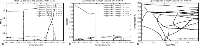
Step calculation. Results from the STEP calculation presented by GNUPLOT for a six-component high speed steel at varying temperature, (a) the amount of phases, (b) mass fraction of Cr in the different phases, and (c) the phase diagram.

Plans for future features include
-
New models for unaries for proper utilisation of results from DFT calculations [33,34,56-60].
-
Module for the assessment of model parameters.
-
Implementation of a corrected quasichemical model for liquid [63].
Interested readers are encouraged to download the current version [61] and give feedback to the developers or participate in further development. It is important that the developers receive feedback from users who are willing to take the time to test this version.
Desirable future developments beyond open source code
It was previously mentioned that no method for uncertainty quantification of the results from the CALPHAD calculations is currently available. The first logical step in this direction is to perform a sensitivity analysis of the model parameters that are being adjusted during the optimization of the thermodynamic description of a binary or ternary system.
In addition to uncertainty quantification, it is desirable to develop a set of test cases to ensure that the results are consistent with accepted codes. Although the results from calculations should agree once the convergence criteria are fulfilled, it is not always guaranteed that the true set of equilibrium phases has been found. Although grid minimizers are intended to assure that the true equilibrium is found, the reliability of these results will depend on how the grid was established.
The development of tools for uncertainty quantification, verification, and validation requires a transparent code that can be easily modified to accommodate the required tests. The availability of an open source code is essential to address these needs and opens the door for future development and improvement of the CALPHAD method and for further integration with materials and process simulation tools.
References
National Science and Technology Council (2011) Materials genome initiative for global competitiveness, Office of Science and Technology Policy, Washington, DC.
National Research Council, Committee on Integrated Computational Materials Engineering (2008) Integrated computational materials engineering: a transformational discipline for improved competitiveness and national security, National Research Council, Committee on Integrated Computational Materials Engineering, Washington, DC.
Olson GB (2014) Preface to the viewpoint set on: The Materials Genome. Scripta Mater 70: 1–2.
Kattner UR, Eriksson G, Hahn I, Schmid-Fetzer R, Sundman B, Swamy V, Kussmaul A, Spencer PJ, Anderson TJ, Chart TG, Costa e Silva A, Jansson B, Lee B-J, Schalin M (2000) Use of thermodynamic software in process modelling and new applications of thermodynamic calculations. Calphad 24: 55–94.
Olson G (2013) Genomic materials design: The ferrous frontier. Acta Mater 61: 771–781.
Hickel T, Kattner UR, Fries SG (2014) Computational thermodynamics: Recent developments and future potential and prospects. Phys Status Solidi B 251: 9–13.
Olson GB (1997) Computational design of hierarchically structured materials. Science 277: 1237–1242.
Reed RC, Tao T, Warken N (2009) Alloys-by-design: application to nickel-based single crystal superalloys. Acta Mater 57: 5898–5913.
Xu W, Rivera-Díaz-del-Castillo PEJ, van der Zwaag S (2008) Genetic alloy design based on thermodynamics and kinetics. Phil Mag 88: 1825–1833.
Gheribi AE, Robelin C, Le Digabel S, Audet C, Pelton AD (2011) Calculating all local minima on liquidus surfaces using the FactSage software and databases and the mash adaptive direct search algorithm. J Chem Thermodyn 43: 1323–1330.
Tancret F (2013) Computational thermodynamics, Gaussian processes and genetic algorithms: combined tools to design new alloys. Modelling Simul Mater Sci Eng 21: 045013.
Saunders N, Kucherenko S, Li X, Miodownik AP, Schille J-P (2001) A new computer program for predicting materials properties. J Phase Equilib 22: 463–469.
JMatPro Practical Software for Materials Properties. http://www.sentesoftware.co.uk/jmatpro.aspx.. Accessed 19 December 2014.
Shobu K (2009) CaTCalc: New thermodynamic equilibrium calculation software. Calphad 33: 279–287.
Bale CW, Bélisle E, Chartrand P, Decterov SA, Eriksson G, Hack K, Jung I-H, Kang Y-B, Melançon J, Pelton AD, Robelin C, Petersen S (2009) FactSage thermochemical software and databases - recent developments. Calphad 33: 295–311.
MatCalc The Materials Calculator. http://matcalc.tuwien.ac.at/.. Accessed 19 December 2014.
Davies RH, Dinsdale AT, Gisby JA, Robinson JAJ, Martin SM (2002) MTDATA - thermodynamic and phase equilibrium software from the national physical laboratory. Calphad 26: 229–271.
Cao W, Chen S-L, Zhang F, Wu K, Yang Y, Chang YA, Schmid-Fetzer R, Oates WA (2009) The Pandat software with PanEngine, PanOptimizer and PanPrecipitation for multi-component phase diagram calculation and materials property simulation. Calphad 33: 328–342.
Andersson J-O, Helander T, Höglund L, Shi P, Sundman B (2002) Thermo-Calc & DICTRA, computational tools for materials science. Calphad 26: 273–312.
Shi P, Engström A, Sundman B, Ågren J (2011) Thermodynamic calculations and kinetic simulations of some advanced materials. Mater Sci Forum675-677: 961–974.
Liu Z-K, Chen L-Q, Raghavan P, Du Q, Sofo JO, Langer SA, Wolverton C (2004) An integrated framework for multi-scale materials simulations and design. J Comput-Aided Mater Des 11: 183–199.
Liu Z-K, Chen L-Q, Krishna R (2006) Linking length scales via materials informatics. JOM 58(11): 42–50.
Grafe U, Böttger B, Tiaden J, Fries SG (2000) Coupling of multicomponent thermodynamic databases to a phase field model: application to solidification and solid state transformations of superalloys. Scripta Mater 42: 1179–1186.
Schneider MC, Gu JP, Beckermann C, Boettinger WJ, Kattner UR (1997) Modeling of micro- and macrosegregation and freckle formation in single-crystal nickel-base superalloy directional solidification. Metall Mater Trans A28A: 1517–1531.
Banerjee DK, Samonds MT, Kattner UR, Boettinger WJ (1997) Coupling of phase diagram calculations for muliticomponent alloys with solidification micromodels is casting simulation software. In: Beech J Jones H (eds)Solidification Processing 1997: Proceedings of the 4th Decennial International Conference on Solidification Processing, 354–357, Department of Engineering Materials, University of Sheffield, Sheffield.
Warnken N, Ma D, Dreverman A, Reed RC, Fries SG, Steinbach I (1997) Phase-field modeling of as-cast microstructure evolution in nickel-based superalloys. Acta Mater 57: 5862–5875.
10 Reasons Open Source Is Good for Business. http://www.pcworld.com/article/209891/. Accessed 19 December 2014.
Ince DC, Hatton L, Graham-Cumming J (2012) The case for open computer programs. Nature 482: 485–488.
GEM Software (GEMS) Home. http://gems.web.psi.ch.. Accessed 19 December 2014.
MELTS Home Page. http://melts.ofm-research.org/.. Accessed 8 December 2014.
Cool T, Bartol A, Kasenga M, Modi K, García RE (2010) Gibbs: Phase equilibria and symbolic computation of thermodynamic properties. Calphad 34: 393–404.
Snider J, Griva I, Sun X, Emelianenko M (2015) Set based framework for Gibbs energy minimization. Calphad 48: 18–26.
Gonze X, Beuken J-M, Caracas R, Detraux F, Fuchs M, Rignanese G-M, Sindic L, Verstraete M, Zerah G, Jollet F, Torrent M, Roy A, Mikami M, Ghosez P, Raty J-Y, Allan DC (2002) First-principles computation of material properties: the ABINIT software project. Comput Mater Sci 25: 478–489.
Giannozzi P, Baroni S, Bonini N, Calandra M, Car R, Cavazzoni C, Ceresoli D, Chiarotti GL, Cococcioni M, Dabo I, Dal Corso A, de Gironcoli S, Fabris S, Fratesi G, Gebauer R, Gerstmann U, Gougoussis C, Kokalj A, Lazzeri M, Martin-Samos L, Marzari N, Mauri F, Mazzarello R, Paolini S, Pasquarello A, Paulatto L, Sbraccia C, Scandolo S, Sclauzero G, Seitsonen AP, et al (2009) Quantum ESPRESSO: a modular and open-source software project for quantum simulations of materials. J Phys: Condens Matter 21: 395502.
OpenPhase. http://www.openphase.de/.. Accessed 19 December 2014.
Guyer JE, Wheeler D, Warren JA (2009) FiPy: partial differential equations with Python. Comput Sci Eng 11(3): 6–15.
Langer SA, Fuller Jr ER, Carter WC (2001) OOF: an image-based finite-element analysis of materials microstructures. Comput Sci Eng 3(3): 15–23.
Eriksson G, Sippola H, Sundman B (1994) A proposal for a general thermodynamic calculation interface. In: Jokilaakso A (ed)1st Colloquium on Process Simulation, 67–103.. Helsinki University of Technology, Helsinki.
TQ-Interface Programmer’s Guide. http://www.thermocalc.com/support/documentation/. Accessed 19 December 2014.
Steinbach I, Böttger B, Eike J, Warnken N, Fries SG (2007) CALPHAD and phase-field modeling: a successful liaison. J Phase Equilib Diffus 28: 101–106.
Kitashima T (2008) Coupling of the phase-field and CALPHAD methods for predicting multicomponent, solid-state phase transformations. Phil Mag 88: 1615–1637.
Xiong H, Huang Z, Wu Z, Conway PP (2011) A generalized computational interface for combined thermodynamic and kinetic modeling. Calphad 35: 391–395.
Lukas HL, Fries SG, Sundman B (2007) Computational Thermodynamics, the Calphad Method. Cambridge Univ. Press, Cambridge.
Sundman B (1981) Application of computer techniques on the treatment of the thermodynamics of alloys. PhD thesis, KTH Stockholm, Sweden.
Hillert M (1981) Some viewpoints on the use of a computer for calculating phase diagrams. Physica103B: 31–40.
Jansson B (1984) Computer operated methods for equilibrium calculations and evaluation of thermochemical model parameters, PhD thesis, KTH Stockholm, Sweden.
Lukas HL, Weiss J, Henig E-T (1982) Strategies for the calculation of phase diagrams. Calphad 6: 229–251.
Chen S-L, Chou K-C, Chang YA (1993) On a new strategy for phase diagram calculation. 1. basic principles. Calphad 17: 237–250.
Chen S-L, Chou K-C, Chang YA (1993) On a new strategy for phase diagram calculation. 2. binary systems. Calphad 17: 287–302.
Thermo-Calc Database Manager’s Guide. http://www.thermocalc.com/support/documentation/. Accessed 19 December 2014.
NIST Repositories. http://nist.matdl.org/, https://materialsdata.nist.gov/dspace/xmlui.. Accessed 19 December 2014.
Bratberg J, Mao H, Kjellqvist L, Engström A, Mason P, Chen Q (2012) The development and validation of a new thermodynamic database for Ni-based alloys. In: Huron ES, Reed RC, Hardy MC, Mills MJ, Montero RE, Portella PD, Telesman J (eds)Superalloys 2012: 12 Th International Symposium on Superalloys, 803–812.. TMS (The Minerals, Metals & Materials Society), Warrendale, PA.
Palumbo M, Fries SG, Hammerschmidt T, Abe T, Crivello J-C, Al Hasan Breidi A, Joubert J-M, Drautz R (2014) First-principles based phase diagrams and thermodynamic properties of tcp phases in Re-X systems (X = Ta, V, W). Comput Mater Sci 81: 433–445.
Lejaeghere K, Van Speybroeck V, Van Oost G, Cottenier S (2014) Error estimates for solid-state density-functional theory predictions: an overview by means of the ground-state elemental crystals. Crit Rev Solid State Mater Sci 39: 1–24.
Campbell CE, Kattner UR, Liu Z-K (2014) The development of phase-based property data using the CALPHAD method and infrastructure needs. Integr Mater Manuf Innov 3: 12.
Palumbo M, Burton B, Costa e Silva A, Fultz B, Grabowski B, Grimvall G, Hallstedt B, Hellman O, Lindahl B, Schneider A, Turchi PEA, Xiong W (2014) Thermodynamic modelling of crystalline unary phases. Phys Status Solidi B 251: 14–32.
Becker CA, Ågren J, Baricco M, Chen Q, Decterov SA, Kattner UR, Perepezko JH, Pottlacher GR, Selleby M (2014) Thermodynamic modelling of liquids: CALPHAD approaches and contributions from statistical physics. Phys Status Solidi B 251: 33–52.
Körmann F, Al Hasan Breidi A, Dudarev SL, Dupin N, Ghosh G, Hickel T, Korzhavyi P, Muñoz JA, Ohnuma I (2014) Lambda transitions in materials science: recent advances in CALPHAD and first-principles modelling. Phys Status Solidi B 251: 53–80.
Hammerschmidt T, Abrikosov IA, Alfè D, Fries SG, Höglund L, Jacobs MHG, Koßmann J, Lu X-G, Paul G (2014) Including the effects of pressure and stress in thermodynamic functions. Phys Status Solidi B 251: 81–96.
Rogal J, Divinski SV, Finnis MW, Glensk A, Neugebauer J, Perepezko JH, Schuwalow S, Sluiter MHF, Sundman B (2014) Perspectives on point defect thermodynamics. Phys. Status Solidi B 251: 96–129.
OpenCalphad. http://www.opencalphad.org/. https://github.com/sundmanbo/opencalphad.. Accessed 19 December 2014.
Hillert M, Jansson B, Sundman B, Ågren J (1985) A two-sublattice model for molten solutions with different tendency for ionization. Metall Trans A16A: 261–266.
Hillert M, Selleby M, Sundman B (2009) An attempt to correct the quasichemical model. Acta Mater 57: 5237–5244.
Acknowledgements
Funding by the Interdisciplinary Centre for Advanced Materials Simulation (ICAMS), which is supported by ThyssenKrupp AG, Bayer MaterialScience AG, Salzgitter Mannesmann Forschung GmbH, Robert Bosch GmbH, Benteler Stahl/Rohr GmbH, Bayer Technology Services GmbH, and the state of North-RhineWestphalia as well as the European Commission in the framework of the European Regional Development Fund (ERDF). One of the developers, BS, is grateful for a Humboldt senior research award.
NIST does not endorse any commercial products, and use of these products does not imply endorsement by NIST.
Author information
Authors and Affiliations
Corresponding author
Additional information
Competing interests
The authors declare that they have no competing interests.
Authors’ contributions
BS and URK contributed the majority to the present article. MP and SGF contributed in the formalism development and discussed and contributed to the present article. All authors read and approved the final manuscript.
Rights and permissions
Open Access This article is distributed under the terms of the Creative Commons Attribution 4.0 International License (https://creativecommons.org/licenses/by/4.0), which permits use, duplication, adaptation, distribution, and reproduction in any medium or format, as long as you give appropriate credit to the original author(s) and the source, provide a link to the Creative Commons license, and indicate if changes were made.
About this article

Cite this article
Sundman, B., Kattner, U.R., Palumbo, M. et al. OpenCalphad - a free thermodynamic software. Integr Mater Manuf Innov 4, 1–15 (2015). https://doi.org/10.1186/s40192-014-0029-1
Received:
Accepted:
Published:
Issue Date:
DOI: https://doi.org/10.1186/s40192-014-0029-1