Abstract
Grid-scale energy storage systems are of interest as the world increases reliance on renewable energy sources. Redox flow batteries are a type of grid-scale energy storage technology that shows exceptional promise for accommodating the dynamic output of wind and solar power sources. The research community employs dozens of diagnostic techniques to investigate nearly all facets of these devices. Material properties, operational losses, transport, and integrated system properties are studied through the lens of electrochemical, physical, and chemical phenomena that ultimately dictate cost by influencing efficiency, durability, power, and capacity. These diagnostic techniques can, if applied correctly, elucidate not only the types of losses in redox flow batteries, but also tie those losses to fundamental driving forces in such systems so that next generation systems and models can be designed. This review details various diagnostic techniques used in flow battery analysis. The benefits, unique insights, and limitations of these techniques are discussed. Recommendations are also made to assist researchers in identifying the diagnostics that can advance their particular investigations. The review concludes with a summary of opportunities for new diagnostics that are needed to enable solution of persistent issues in redox flow battery research and development.
Export citation and abstract BibTeX RIS

This is an open access article distributed under the terms of the Creative Commons Attribution 4.0 License (CC BY, http://creativecommons.org/licenses/by/4.0/), which permits unrestricted reuse of the work in any medium, provided the original work is properly cited.
The successful implementation of renewable energy sources to the electric grid requires robust energy storage systems. Grid scale energy storage systems are being developed at a higher rate than ever before and are available in multiple technological formats. There, is of yet, no superior energy storage option for all types of applications since technologies vary in terms of performance characteristics, capital requirements, maturity level, lifetime, safety, reliability and the level of environmental and human risks. A comprehensive analysis of different storage technologies is available in a recent report from Sandia National Laboratory.1 There are several electrochemical-energy-based storage technologies including redox flow batteries (RFBs), non-flowing secondary batteries, regenerative fuel cells (RFCs), rechargeable metal-air batteries, supercapacitors and many others. Several review papers have discussed these technologies in greater detail (e.g.).2–5
Among the available storage technologies, RFBs have been a recent focus of interest. RFBs belong to the family of secondary batteries and have two broad categories: all-liquid and hybrid phase batteries. The hybrid phase RFBs has three main categories including gas/liquid, solid/liquid and semi-solid phases. For semi-solid hybrid RFBs, energy-dense solid particles are suspended within the liquid electrolyte. In terms of operation, all-liquid RFBs differ from conventional batteries since the electrodes themselves typically do not undergo any faradaic reaction. In hybrid RFBs, faradaic reactions can occur at solid electrodes which are typically paired with liquid- or gas-phase electrodes.
All-liquid RFBs boast the advantage of decoupling energy storage capacity from power capacity, because the electroactive redox couples are stored in external reservoirs and brought together in the reactor during operation. The storage of solutions in reservoirs separated from the reactor provides RFBs with unique benefits compared to other secondary batteries: safety is improved by minimizing the potential to short circuit; state of charge (SoC) monitoring can be done directly on the solution reservoirs, improving system control; and crossover can be significantly curtailed. Some other properties of RFBs include relatively long cycle life and the possibility of rapid mechanical charging.3,6,7 RFBs do have relatively low energy density, largely preventing their use in mobile applications.
Like some other secondary batteries, RFBs utilize reversible anodic and cathodic redox reactions of soluble species within the electrolyte. The negative and positive electrolytes are pumped inside the reactor where the half-cell electrochemical reactions occur. The generic half-cell reactions can be formulated as follows, assuming an n electron transfer process for the redox reactions.
![Equation ([1])](https://content.cld.iop.org/journals/1945-7111/165/5/A970/revision1/d0001.gif)
![Equation ([2])](https://content.cld.iop.org/journals/1945-7111/165/5/A970/revision1/d0002.gif)
![Equation ([3])](https://content.cld.iop.org/journals/1945-7111/165/5/A970/revision1/d0003.gif)
Equation 1 is the negative half-cell reaction and Eq. 2 demonstrates the positive half-cell reaction; together they compose the overall cell reaction (Eq. 3) with the maximum theoretical cell potential of E0cell at standard conditions.
Myriad chemistries have been proposed and investigated for RFBs, with the primary differences being which compounds, organic or inorganic, carry charge in aqueous or non-aqueous solutions. Table I includes many of the predominant types of RFBs under development. The choice of electro-active redox couple depends on the particular application but ultimately is determined based on many factors, overall cost of the redox flow battery system being one of the strongest. The Department of Energy (DOE) has set a target cost of $250/kWh for short-term grid storage system capital cost; $150/kWh is the long-term goal.8 Moreover, the Advanced Research Projects Agency-Energy (ARPA-E) Grid-Scale Rampable Intermittent Dispatchable Storage (GRIDS) program has proposed the more aggressive cost target of $100/kWh.9 One methodology for determining the total energy storage cost in the system level has been discussed using a performance-based cost model developed at Pacific National Laboratory (PNNL).10,11 It has been shown via model prediction that the overall system level cost is not only a function of the electroactive material selection, but also the stack design, performance, and operating conditions. In order to achieve the aggressive cost targets determined by DOE for widespread commercialization of RFBs, decreasing the system material costs and increasing the cell performance are the logical pathways.7,12 Recently, a hybrid aqueous sulfur/sodium/air RFB has been demonstrated in the laboratory scale with the chemical cost of only $1/kWh opening a door toward achieving the cost target assigned by DOE.13 In addition, a zinc-iron (Zn-Fe) RFB with double-membrane triple-electrolyte design has been demonstrated with an estimated system capital cost of under $100/kWh.14
Table I. Different Varieties of RFBs.
| Negative electrolyte | Positive electrolyte | OCV (V) | Ref. | ||||
|---|---|---|---|---|---|---|---|
| All-liquid RFB | Aqueous solvent | Inorganic solutes | All-Vanadium | V(II)/V(III) | V(IV)/V(V) | 1.26 | 15–18 |
| Iron-Chromium | Cr(II)/Cr(III) | Fe(II)/Fe(III) | 1.18 | 19–22 | |||
| Polysulfide-Bromine | Sodium Polysulfide | Sodium Bromide | 1.36 | 3,19 | |||
| Vanadium-Bromine | V(II)/V(III) | Br2/Br− | 1.3 | 23,24 | |||
| Organic solutes | Quinone–Bromide | Quinone/Hydroquinone | Br2/Br− | 0.92 (at SoC = 90%) | 25 | ||
| Anthraquinone - Benzoquinone | AQS/H2AQS | BQDS/H2BQDS | 1.0 | 26 | |||
| Non-aqueous solvent | Inorganic solutes | Zinc-Cerium | Zn | Ce(III)/Ce(IV) | 2.5 | 27 | |
| Ruthenium Complexes | [Ru(bpy)3]2+/[Ru(bpy)3]3+ | [Ru(bpy)3]+/[Ru(bpy)3]2+ | 2.6 | 28 | |||
| Chromium - Acetylacetonate | Cr(I)/Cr(II) |Cr(II)/Cr(III) | Cr(III)/Cr(IV) |Cr(IV)/Cr(V) | 3.4 | 29–31 | |||
| Organic solutes | Anthraquinone | Li metal | Anthraquinone | 2.6 | 32 | ||
| Lithium-based | Li-PAHA | PAHB | 3.0 | 33 | |||
| Quinoxalines | N/A | N/A | N/A | 34,35 | |||
| Hybrid RFB | Solid-Liquid | Zinc-Bromine | Zn/Zn2+ | Br2/Br−/Br3− | 1.67 | 17 | |
| Zinc-Cerium | Zn/Zn2+ | Ce3+/ Ce4+ | 2.4 | 36,37 | |||
| All-Iron | Fe/Fe(II) | Fe(II)/Fe(III) | 1.2 | 38,39 | |||
| All-Lead | Pb(II)/Pb | Pb(II)/PbO2 | 1.78 | 40,41 | |||
| All-Copper | CuCl32−/Cu(s) | CuCl42−/CuCl32− | 0.773 | 42 | |||
| Semi-solid | Lithium-based | Li4Ti5O12 | LiCoO2 | 4.5 | 43 | ||
| Gas-Liquid | Hydrogen-Bromine | H2/H+ | Br2/Br− | 1.09 | 44,45 | ||
| Vanadium-Oxygen | V(II)/V(III) | H2O/O2 | 1.49 | 46–48 | |||
| Hydrogen-Vanadium | H2/H+ | V(IV)/V(V) | 0.99 | 49,50 | |||
| Sulfur-Sodium-Air | Polysulfide | Air | 1.5 | 13 | |||
The main objective of this review is to discuss the available experimental techniques to diagnose cell behavior, identify limitations of the existing diagnostics, and provide perspectives of the future needs of the field so that high performance systems meeting DOE cost and performance goals can be achieved. These diagnostic techniques can largely be applied to any material (chemistry) of interest, though some may carry increased complications in some systems.
The all-liquid RFBs are types in which the electroactive species are dissolved in a solvent to constitute the anolyte and catholyte solutions. The most common solvent is water; usually, some supporting electrolyte is added to adjust pH and increase conductivity and solubility. Aqueous solvents are typically limited by the water electrolysis potential window (The recorded onset potential for water splitting is 1.26 V and 1.48 V, depending on the presence of liquid and/or vapor water phase at the electrocatalyst-electrolyte interface)51 and the low solubility and stability of the electroactive species within the electrolyte. Non-aqueous solvents are also available for all-liquid RFBs. In general, non-aqueous electrolytes enable a wider operational potential window but at the cost of increased solvent cost, viscosity and ionic resistivity. More details regarding non-aqueous solvents are available through a relatively recent review paper in which comparisons are provided with reference to aqueous solvents.52 The electroactive species in all-liquid RFBs can be inorganic (mostly metals) or organic materials. The application of organic electroactive species is favorable because of generally lower cost and increased solubility.25,53–60 Recent developments in organic redox flow batteries have been reviewed in Ref. 61 focusing on the chemistry, redox potentials, solubility, stability and materials perspectives.
Hybrid batteries can be split into three main categories: solid/liquid, semisolid, and gas/liquid forms. For solid/liquid hybrid batteries, the solid species deposits on an electrode. Dendrite formation at high current and surface passivation are usually limiting factors, especially for system lifetime. In order to overcome this issue, semisolid RFBs show promise. The semisolid RFBs, demonstrated by Chiang et al.,43 utilize conductive materials that are suspended in solution and pumped inside the reactor.43,62,63 Gas/liquid hybrid batteries utilize a half-cell reaction involving gaseous species.
As summarized in Table I, there are many types of RFBs under development, with new chemistries frequently introduced and a rising interest in organic and/or non-aqueous solvents. Here, we included the most-investigated types of RFBs; we refer readers to other review papers that discuss the different types summarized in Table I in greater detail (e.g.).3,6,7,52,64–70
Performance improvements have been demonstrated recently for all-vanadium71–73 and hydrogen-bromine cells74–79 with these chemistries still requiring optimization in order to approach the DOE cost target goal. RFB optimization is usually performed at the component level for any established chemistry. Figure 1 is a schematic of a generic RFB. In general, a redox flow battery system includes the storage reservoirs (gas and/or liquid), electrochemical reactor, pumping system, temperature control system, and power control unit.
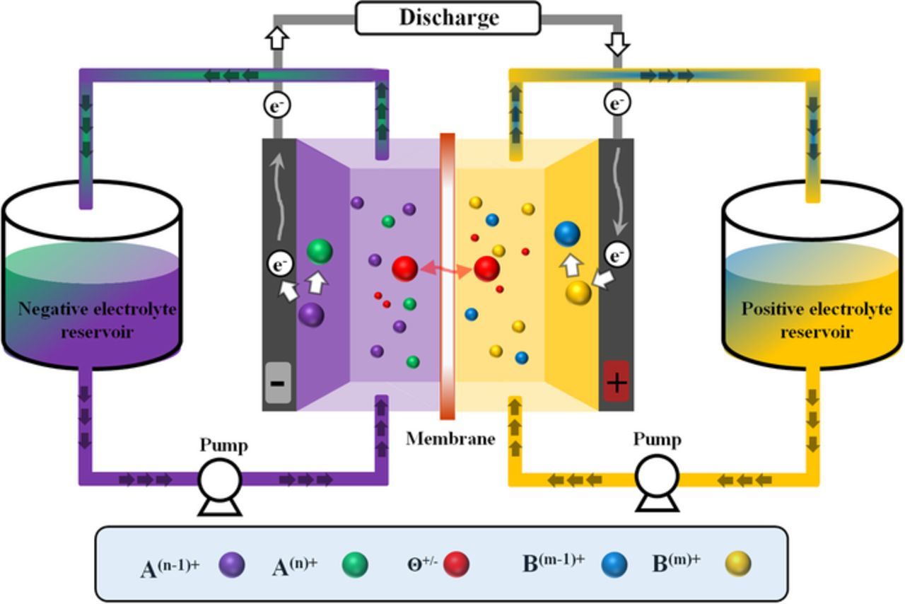
Figure 1. Schematic representation of a single-cell RFB.
The reactor depicted in Fig. 1 is the most important part of the RFB system where energy conversion (between chemical and electrical) occurs. In general, the reactor includes the separator (with the exception of membrane-less RFBs),80 porous electrodes, gaskets, flow plates, current collectors and endplates. In practical applications, an arrangement of parallel stacks of multiple reactors is used to achieve the desired power/voltage of the system. Figure 2 includes exploded views of a single cell as well as of a stack.
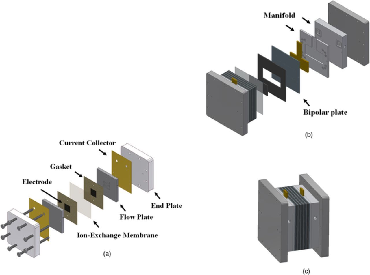
Figure 2. Schematic representation of single-cell and stacked RFBs (a) Exploded view of a single cell, (b) Exploded view of stack of multiple cells, (c) schematic of the assembled stack of multiple cells).
The ion-exchange membrane (separator) in the reactor separates the anode and cathode sides; an ideal separator must have high ionic conductivity, very low permeability for the electroactive species, chemical and thermo-mechanical stability, and low cost. For many RFB systems, the separator is the most expensive single component, comprising 30–40% of the reactor's cost.10 Nafion is a widely-used separator for aqueous RFBs and polymer electrolyte fuel cell systems (PEFC). More detailed information about Nafion membranes is available elsewhere (e.g.).81 Recent progress on separator development for vanadium RFBs has been summarized.82,83 Although Nafion has successfully been used for aqueous RFBs, its application for non-aqueous RFBs faces considerable challenges. Shin et al. has recently reviewed the application of different separators for non-aqueous RFBs.84
Porous electrodes are used to provide high surface area for electroactive species redox reactions. The electrodes must also have high electrical conductivity and electrochemical stability. Electrode morphology directly affects transport of electroactive species and the surface chemistry of the electrodes can provide catalytic support for redox reactions on one or both sides of a RFB. The application of disparate electrode materials for each half of a particular RFB has been discussed in multiple review papers.64,85 The most common electrode materials are partially or fully-graphitized carbon in the form of paper or felt.
Flow plates in RFBs serve to distribute the electrolyte across the electrodes in each single cell while also functioning as bipolar plates in stacks. The flow plates should have high electrical conductivity and electrochemical stability and, at the same time, effectively-zero fluid permeability. Flow plates are often modified forms of graphite; many forms of graphite are porous; thus some sealing treatment is typically done to prevent electrolyte leakage through the flow plates. In general, there are two types of common configurations adopted for the flow plates (Fig. 3). In the first configuration (flow-frame architecture), the flow plates include electrolyte inlet and outlet ports with an optional gap in the top and bottom sections leading into and out of the electrode.86 In the second configuration (flow-channel architecture), porous electrodes are pressed against flow plates that have a channel pattern and geometry. A review of different flow plate architectures is available in the review paper of X. Li et al.87
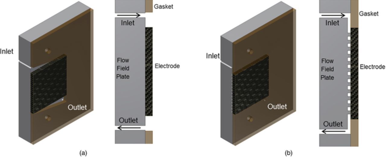
Figure 3. Flow plate configurations. (a) flow-frame architecture, (b) flow-channel architecture).
The selection of gasket materials for any specific RFB is based on compressibility and material compatibility with regard to electrolytes. Teflon PTFE (DuPont Corporation) and Viton (DuPont Corporation) are among the common choices for gasket materials.
The current collectors are only at the end of a stack of cells; they are typically manufactured from very conductive materials (Au or Cu), plated onto aluminum (usually for lab-scale cells), and are electronically isolated from the endplates.
Figures 2 and 3 are only the most common reactor configurations for RFB systems. Membrane-less RFBs have attracted attention and are the focus of some research.80,88–90 Membrane-less RFBs avoid the high cost of a separator, but have only been demonstrated at low Reynolds numbers (Re < 10) which reduces mixing of electrolytes. In membrane-less RFBs, two laminar electrolyte streams flow in a co-flow configuration, side-by-side (Fig. 4), through the reactor. The membrane-less RFB variant is reviewed in Ref. 80. The most popular chemistries for membrane-less flow batteries are all-vanadium,91 hydrogen-bromine,90 zinc-bromine,92 and Au based systems.93 The concept of membrane-less RFBs is similar to the membrane-less microfluidic fuel cells introduced years earlier.94,95
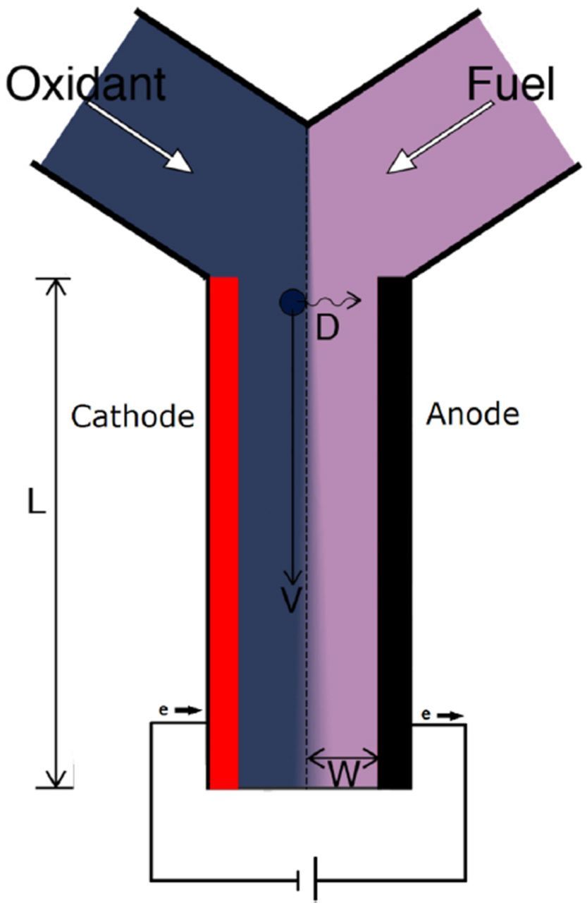
Figure 4. Schematic of membrane-less RFB (picture is taken from Ref. 80).
Although membrane-less RFBs can significantly decrease the cost of RFBs by eliminating the ion-exchange membranes, their application is mostly limited to low-power. Scale-up issues need to be solved before a transition to medium- or high-power can occur. Recently, Braff et al. demonstrated a promising hydrogen-bromine membrane-less flow battery that maintained voltage efficiency above 80% as high as ∼350 mW/cm2 (Fig. 5).90
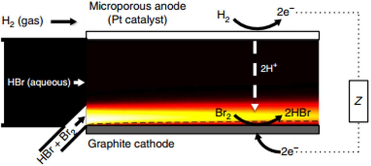
Figure 5. Schematic of HBr membrane-less RFB (picture is taken from Ref. 90).
As the variety of chemistries continues to grow, the process of designing a high-performance RFB system becomes increasingly complex. Recently, online material databases and computational screening techniques have been the focus of attention for electrolyte material discovery and selection.96,97 One of the successful implementations of these techniques is the Electrolyte Genome project.98 The Electrolyte Genome project has been designed to aid in the selection of battery electrolyte materials based on calculations of molecular properties.98 It is also important to note that the investigation of appropriate materials for optimum electrolyte must be followed by a further analysis for improved electroactive ions solubility and stability (chemical and thermal) for long-term cycling. An example of such an analysis is provided recently in a review paper focused for the various types of electrolytes to be used for VRFBs.99
Upon finalizing the configuration along with the desired chemistry, performance improvement using multiple diagnostic techniques can be achieved through detailed understanding of localized inefficiencies. Further details are available regarding engineering aspects of the design and performance of RFBs in a recent review paper as described in Ref. 100.
Mathematical models are also being developed alongside diagnostic techniques to enhance the optimization process and provide deeper insights. Mathematical models have been developed for different RFB systems with varying levels of complexity. The focus of this review is on experimental diagnostics, thus modeling efforts are not emphasized here. A focused review of RFBs including modeling efforts and can be found elsewhere.101
Performance metrics or figures of merit provide quantitative values to judge RFB performance from multiple perspectives. The most frequently-used figures of merit include voltage efficiency, coulombic efficiency, system level energy efficiency, theoretical capacity utilization and discharge capacity fade over long-term cycling.
Voltage efficiency
The ratio of cell voltage during discharge and charge processes is defined as the voltage efficiency, shown in Equation 4.3
![Equation ([4])](https://content.cld.iop.org/journals/1945-7111/165/5/A970/revision1/d0004.gif)
Where the VcellDchg and VcellChg represent the average cell voltage during discharging and charging, respectively, at a certain time or desired SoC. For these measurements, current density is typically held constant. At any particular current density, there are multiple sources of overvoltage including kinetic, ohmic, and mass transport losses which result in decreased voltage efficiency. All three sources of loss increase with current density, though not with the same dependence.
Coulombic efficiency
The ratio of total electrical charge withdrawn during discharge versus the charge stored after charging is defined as coulombic efficiency, as shown in Equation 5.3
![Equation ([5])](https://content.cld.iop.org/journals/1945-7111/165/5/A970/revision1/d0005.gif)
where the QtotalDchg and QtotalChg represent the total electrical charge (in C or A-hr) during discharge and charge processes, respectively, and IDchg and IChg represent the discharge and charge currents (A). There are multiple contributors to coulombic losses including crossover of electroactive species and side reactions. The coulombic losses can be reversible or irreversible depending on the reaction and nature of the electroactive species.
System level energy efficiency
The voltage and coulombic efficiencies represent composite losses at the single cell level and include kinetic, ohmic, mass transport, crossover, and side reaction losses. However, there are other sources of losses when considering the overall RFB system shown in Fig. 1. Parasitic losses (temperature control, pumping losses, and other auxiliary equipment) are generally the most important in terms of loss magnitude and added expense. In addition to single cell losses, stacks of multiple cells introduce new losses including shunt currents, uneven voltage distribution, and uneven electrolyte distribution among cells. System level energy efficiency is defined to account for these sources of losses that are beyond a single cell level.
Theoretical capacity utilization
The maximum theoretical capacity of a RFB system is based on the amount of total electroactive material within the electrolyte. In aqueous systems, this capacity is determined by electroactive species solubility limits. Ideally, a RFB system would be capable of using all the available capacity. However, voltage limits and the various losses (especially mass transport losses at the system SoC limits) cause the practical utilization to be well below 100%. Capacity utilization strongly influences system cost, especially in the case of RFBs that depend on expensive charge carriers.
Discharge capacity fade over long-term cycling
One of the major drawbacks about different types of RFBs is the relatively rapid discharge capacity fade during long-term cycling. The major reasons for discharge capacity fade during long-term cycling include the undesired crossover of solvent and electroactive species through the ion-exchange membrane, degradation of various cell components, undesired side reactions and precipitation of electroactive species. Discharge capacity fade is an important metric in evaluating the stability and robustness of a particular RFB system in delivering the desired output current density.102
In this review, diagnostic techniques are most broadly categorized as in-situ versus ex-situ. Subdivision to electrochemical, physical, or spectroscopic characterizations is further used. This categorization is shown in Table II with a full description of different techniques provided in the following section.
Table II. Major diagnostic techniques utilized for RFBs.
| Electrochemical | in-situ | Discharge Curves and Cycling |
| Polarization Curves | ||
| Cyclic Voltammetry (CV) | ||
| Current Interruption (CI) | ||
| Electrochemical Impedance Spectroscopy (EIS) | ||
| ex-situ | Cyclic Voltammetry (CV) | |
| Conductivity Measurement | ||
| Rotating Disk Electrode (RDE) | ||
| Physical and Spectroscopic | in-situ | Ultraviolet–visible (UV-Vis) spectroscopy |
| Potential Distribution | ||
| Neutron Radiography (NR) | ||
| Pressure Drop and Energy Analysis | ||
| Current Distribution | ||
| Shunt Current Measurement | ||
| ex-situ | Nuclear Magnetic Resonance (NMR) Spectroscopy | |
| Electron Spin Resonance (EPR) Spectroscopy | ||
| Optical Visualization of Flow Distribution | ||
| Thermal Visualization of Flow Distribution | ||
| Scanning Electron Microscope (SEM) | ||
| Energy Dispersive X-ray Spectroscopy (EDS) | ||
| Raman Spectroscopy | ||
| Brunauer-Emmett-Teller (BET) Method | ||
| X-ray photoelectron spectroscopy (XPS) | ||
| Mass Spectroscopy | ||
| X-ray Tomographic Microscopy (XTM) | ||
| Fourier Transform Infrared Spectroscopy (FTIR) |
Diagnostic Techniques
Discharge curves and cycling
Perhaps the most widely-used method for basic characterization of flow battery performance is constant-current discharge and/or charge curves. When charging and discharging curves are executed in series, cycling performance can be assessed. Ultimately, constant current cycling provides the evidence of improvement resulting from materials, design, and operational innovations. Equations 4 and 5 define voltage and coulombic efficiencies, both of which depend on operating current and are drawn from cycling experiments. The energy efficiency is simply the product of the voltage and coulombic efficiencies, also called round-trip energy efficiency in a battery system (often excluding system losses, e.g. pumps, electronics, etc.). A survey of the specifications provided by the companies active in RFBs shows that commercial flow battery systems operate in the 70–80% round-trip efficiency regime (sometimes including the losses from auxiliary systems), though battery systems can be considered competitive even in the 60–70% energy efficiency range, depending on cost.103 Since voltage efficiency strictly decreases with current while coulombic efficiency generally increases with current (prior to the onset of side reactions), there is often a range of current over which acceptable efficiency can be reached – this range is potentially a design consideration, as evidenced by the redox flow battery cost model developed by the team at Pacific Northwest National Laboratory.10
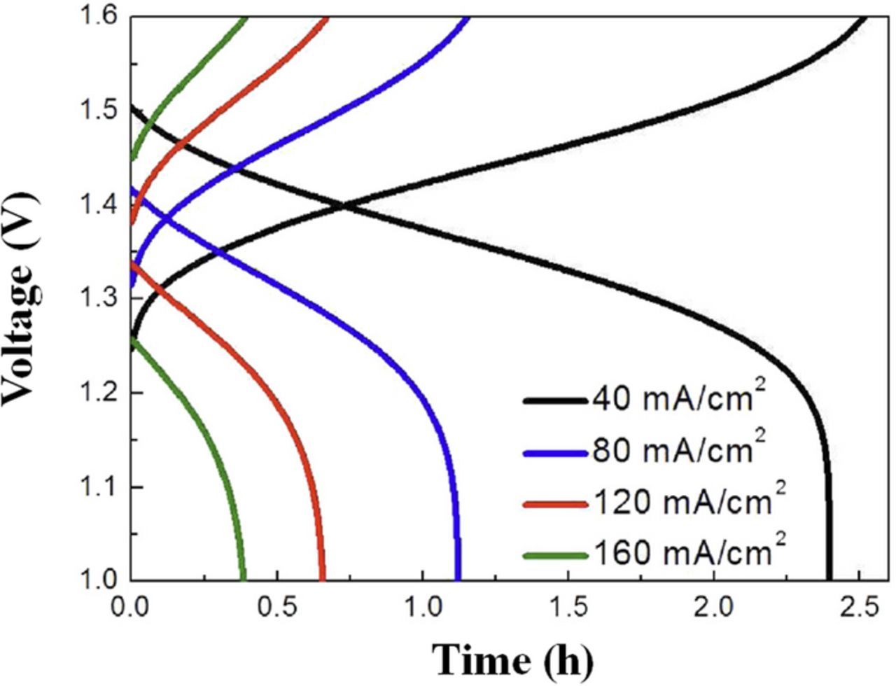
Another metric that can be determined via cycling is the actual charge capacity relative to a theoretical amount that is based on the amount of electroactive species present in a system, often called capacity utilization.104 Capacity utilization is possibly a critical driver of system cost – lower utilization incurs the cost of greater quantities of electroactive species and requires higher storage volume – driving cost up significantly if the electroactive materials strongly influence cost, as in the case of VRFBs.105 Capacity utilization is affected both by current density and by the inherent losses in a cell. Generally, utilization decreases with increasing current density since relatively higher current cannot be supported at the relevant SoC limits.106 An example of the capacity dependence on current density is shown in Fig. 6; here, the greater charge and discharge times correspond to greater capacity utilization at low current density. While voltage efficiency and capacity utilization both decrease with increasing current, achieving the highest current density possible while maintaining acceptable efficiency is the most likely pathway to achieving cost targets for any particular flow battery chemistry.107–112
Cycling is among the simplest diagnostics that can be performed on a flow battery. The cell is alternately charged and discharged at constant current while recording voltage. Assuming the charging and discharging processes are symmetric and that both half-cells are coulombically balanced, the midpoint of each charging or discharging step should be near 50% SoC. This midpoint voltage for both steps is used to calculate the voltage efficiency. The total time for each step is multiplied by the current to obtain the total coulombs passed during a step and then to calculate the coulombic efficiency. Finally, the product of average voltage and coulombs yields the total energy transferred during a step.3
While charge-discharge cycling is practically straightforward, there are numerous behaviors that can be observed, as well as some gaps in what can be learned. In addition to the insights described previously (efficiencies and capacity), the sensitivity of cycling behavior to current density can provide some indirect insight into limiting behaviors in the battery, e.g. slow reaction kinetics, high ohmic loss, and poor mass transport. Since the concentration of reactant species (in VRFB systems, V(IV) and V(III) during charging, V(V) and V(II) during discharging) decreases during a charge or discharge process, consideration of the current and concentration can give additional indirect information on limiting behavior (e.g. kinetics or transport-limited current). Such observations are possible in Fig. 6: at low current, long-duration voltage stability indicates that mass transport is not strongly limiting for most of the step and the polarization behavior of the cell can be predicted using mathematical models (e.g. Butler-Volmer equation); however, at the highest current, the absence of a stable voltage indicates combined ohmic and mass transport losses in addition to the voltage drop expected via the Butler-Volmer equation.113–118 Cycling experiments do offer the most accessible means to induce and study the degradation of novel RFB components in-situ, though this process is relatively slow except for when an experimental set-up is designed to accelerate degradation under realistic conditions.119 One area required to be explored in details in the literature is longer-range cycling experiments to verify durability of components. However, for the majority of RFB chemistries and configurations, such extensive cycling is difficult to justify due to the high cost in terms of materials, equipment, and time.
A drawback to cycling is that it does not readily provide much direct evidence of how specific changes to battery materials or operation affect loss mechanisms, as cycling provides only a composite assessment of performance. In order to quantitatively understand how various improvements (e.g. modified electrodes, new membranes, alternative flow fields, etc.) affect performance beyond the high-level efficiencies and capacity utilization, most investigations include numerous accompanying diagnostics that yield more focused assessment of in-situ phenomena. The merits and limitations of those diagnostics are described in greater detail as follows.
Polarization curves
Polarization curves illustrate the relationship between cell voltage and charging or discharging current. A generalized polarization curve is shown in Fig. 7; its shape is a composite of kinetic losses usually described by the Butler-Volmer model, ohmic losses obeying Ohm's Law, and mass transport losses (also known as concentration polarization) described by local concentration limitation effect on reaction.120–123 At relatively low current, the losses in the cell are primarily attributed to high kinetic overpotential corresponding to sluggish electrochemical reactions. The steep drop in cell voltage at low current before a cell begins to behave as a series ohmic resistor is usually described with kinetics, most typically involving a Butler-Volmer approximation assuming charge-transport rate limited kinetics. This steep drop is tied to overcoming electrochemical activation energy for both electrode reactions. Simple polarization curve measurements have been used to investigate reaction kinetics in VRFBs and yield similar insights as those gleaned through other in-situ methods.124–127 Additionally, it has been shown in several studies that kinetically-controlled behavior can be largely alleviated in VRFBs via addition of catalysts, treating the electrodes (via thermal or chemical treatment) or by increasing the electrode surface area.128–131
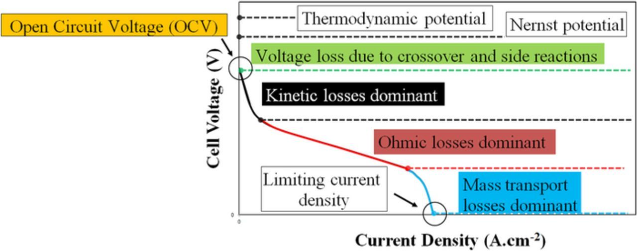
Figure 7. Generalized polarization curve for an electrochemical power conversion device with multiple sources of overpotential.
At intermediate current density, the polarization curve illustrates a linear relationship between current and voltage. The slope of this straight line is proportional to the sum of all internal resistances in the cell. While these resistances include electrical conductivities of external wires, current collectors, flow fields, electrodes, all contacts between those components, and ionic resistance of the electrolyte within the electrodes, ohmic loss is generally dominated by the ionic resistance of the membrane, particularly for thicker membranes that inhibit electroactive materials' crossover.132–134 Strategies to improve contact resistance, which can contribute appreciably to internal resistance when thin membranes are used, generally focus on improved bipolar plate-electrode contact, especially in the case of carbon felt electrodes.135
At the highest currents, concentration polarization may ultimately limit the operation.136 Under these conditions, the cell current is high enough that the electroactive species' diffusion to and from the surface of the electrodes limits cell operation, preventing current from increasing despite increasing overpotential in the cell. It is noted that concentration polarization, as a dominating overpotential, may not be reached for cells with poor kinetics or ohmic losses great enough to drive a cell to the voltage limits before reaching a mass transport-limited current.59 While a polarization curve can be roughly divided into "controlling overpotentials" that are described by fundamental equations, all three components are present at all currents. This behavior prevents polarization curves from definitively correlating an RFB modification to, for example, improved kinetics at the expense of poorer mass transport. Electrochemical impedance spectroscopy (EIS) has been widely used to investigate these contributions based on impedance responses rather than simple, DC voltage-current behavior, providing more confident insight into how controlling overpotentials respond to changes in cell materials or operation;125,130,137,138 these studies and their implications are addressed more fully in the following sections.
Another consideration for polarization curve analysis is that the measurement assumes a constant SoC in the RFB; having been widely used in fuel cells, this assumption was inherently met in those studies. However, assumption of constant SoC may not be appropriate for an RFB in which the electrolyte circulates from and then back to a reservoir for each half cell. Experimental modifications (as shown schematically in Fig. 8) have been described that allow SoC to remain constant in laboratory scale testing, including the cell-in-series method,114,119 symmetric cell operation,114,139 single-pass polarization curves (in which the electrolyte is not recirculated to a single reservoir)106 and alternating charge/discharge currents.
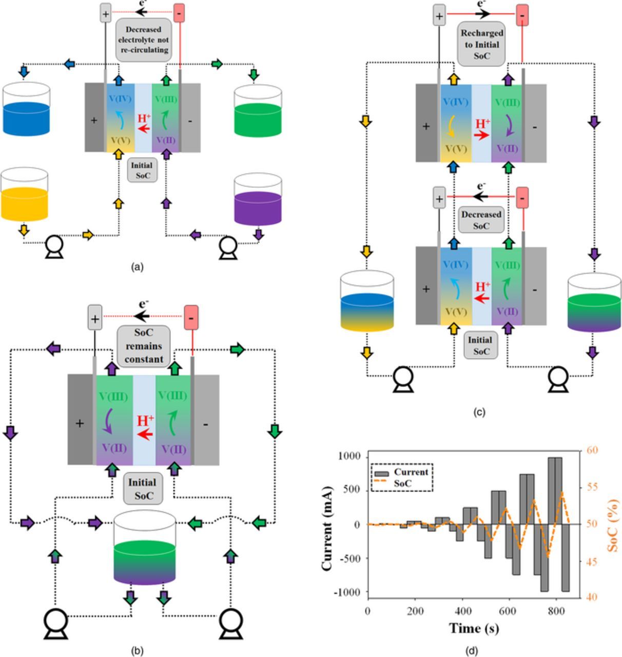
Figure 8. Schematic of the techniques used for operating RFBs under constant state of charge (SoC) condition (a) Single-pass technique, (b) Symmetric cell operation, (c) Cell-in-series method, (d) Alternating charge/discharge current method.
Finally, polarization curves provide no insight regarding coulombic efficiency for a battery.140 Conversely, charge-discharge cycling does not provide the same depth of insight regarding how a cell modification influences operation (via improved kinetics, internal resistance, or mass transport) that polarization curve analysis does. An example of this can be found in an H2/Br flow battery investigation and is shown in Fig. 9.130 Here, BP2000 carbon black was used as a catalyst in an H2/Br flow battery; however, rather than improved kinetics, the catalyst loading more strongly impacted mass transport behavior. In fact, the kinetic performance was impacted more strongly by the type of binder used for the catalyst than by the catalyst itself. Cycling experiments would yield a possible change in voltage efficiency, depending on the cycling current (assuming coulombic efficiency was unchanged). That change would presumably be due to kinetics responding to catalyst loading. The contribution of the polarization curve in this analysis, then, is the insight that mass transport, not kinetics, was most impacted by the catalyst loading. This being the case, polarization curves can be used as an enhancing companion to more common cycling characterization rather than as a replacement to cycling.
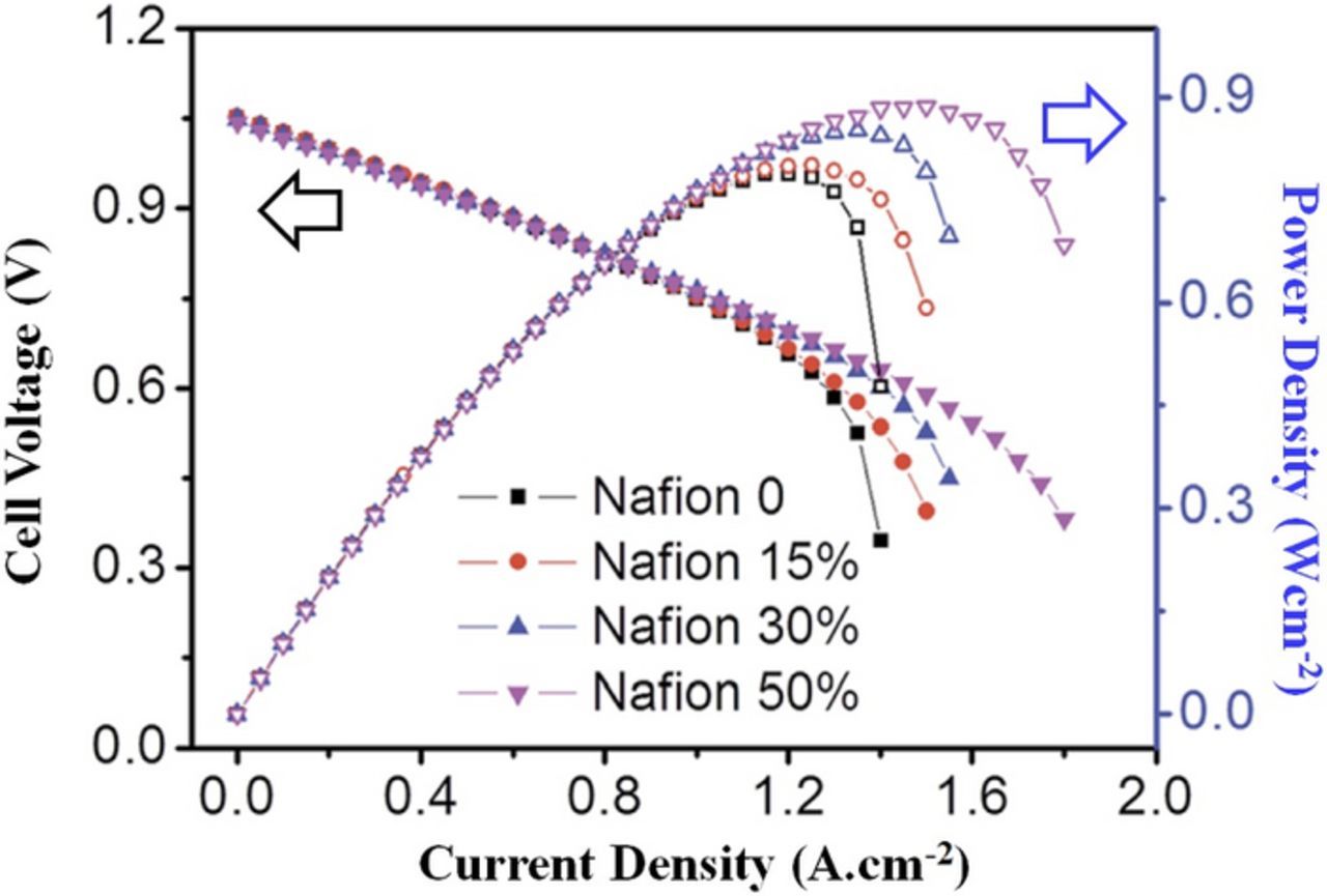
Figure 9. Polarization and power density curves showing the effect of BP2000 loading on H2/Br flow battery (adopted from Ref. 130).
Cyclic voltammetry (CV)
Cyclic Voltammetry (CV) is (typically) an ex-situ electrochemical experiment used to evaluate the current response to a linear voltage sweep. The experiment involves a three electrode set-up (working, counter and reference electrodes), where the working electrode's potential is ramped linearly with respect to time between a relatively negative vertex value and a more positive vertex value multiple times.141,142 The current response is then plotted as a function of the applied voltage sweep in a figure known as a voltammogram. An example of a voltammogram is shown in Fig. 10. This experimental method is commonly used in initial studies of new electrochemical systems.143
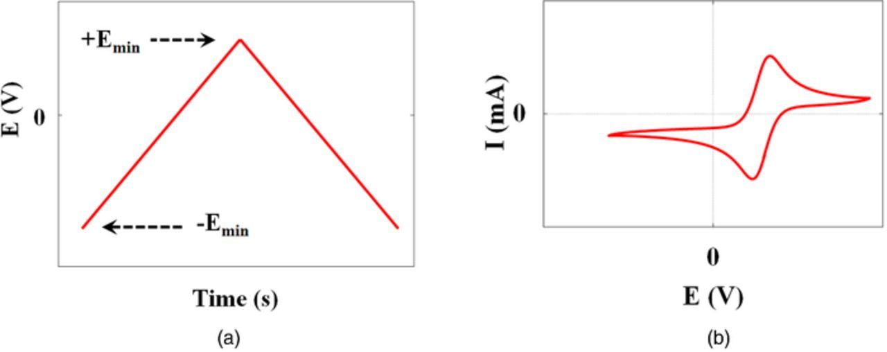
Figure 10. Typical cyclic voltammetry experiment in which (a) working electrode voltage is swept between two vertex potentials over time and (b) the measured current plotted against the control voltage.
An important experimental parameter in CV is voltage scan rate v (V/s). The response of peak current and peak potential separation to scan rate can be indicative of the reversibility of a process. Reversible and quasi-reversible processes have peak currents that are proportional to the square root of scan rate as indicated by the Randles-Sevcik equation.143
![Equation ([6])](https://content.cld.iop.org/journals/1945-7111/165/5/A970/revision1/d0006.gif)
Where ip denotes peak current density, n is the number of electrons transferred in the limiting charge transfer step, A is the electrode area, C0 is the concentration of the reacting species, and D0 is the diffusivity.
While the distinction of being reversible or quasi-reversible can be suggestive of how efficiently electrochemical processes can occur, the primary benefit of this distinction is that there is an abundance of theory that has been developed to diagnose properties of these systems. If a process is reversible or quasi-reversible, a diffusion coefficient and rate constant can be determined. The diffusion coefficient can be determined directly from the Randles-Sevcik equation while a rate constant can be determined from peak current analysis by the Laviron method: a plot of ln(ip) vs. (Ep − E0') has a slope of − αf and an intercept proportional to k0.143
![Equation ([7])](https://content.cld.iop.org/journals/1945-7111/165/5/A970/revision1/d0007.gif)
Where Ep refers to working electrode potential at peak current. k0 is the reaction rate constant and C*o is the concentration of reactive species within the bulk solution.
CV is most frequently used to study electrodes and to compare treatments (catalysts, additive particles)144–148 or other electrode preparation processes (electrochemical).149–152 CV is also commonly used to assess the viability of new electrolyte chemistries31,72,153–159 and has been utilized extensively to assess the performance of various porous electrodes for capacitive deionization.160–162 However, CV is not solely limited to use in studies of kinetics; Small et al.163 used CV to detect chemical species in a membrane crossover study. Common benchmark electrodes utilized in CV include glassy carbon, Pt, and graphite; novel electrode structures and materials are frequently compared to these benchmarks.
Although CV is a very common electrochemical technique, it has several important limitations. First, it can readily portray information about reversibility, but a more in-depth analysis is needed to determine long term stability of products. Another limitation of CV is that the information it provides is often the convolution of multiple experimental components (overpotential including iR loss; faradaic and capacitive current, etc.), this often necessitates very careful analysis or supplementary experiments to obtain accurate, quantitative results.146,149,150 Also, when performing ex-situ experiments, it is important to note the limitations and differences when using electrodes that differ in morphology from those to be used in-situ and how they can behave differently, particularly with respect to surface area and 3D morphology. Indeed, one of the most difficult aspects in obtaining meaningful CV results is replicating realistic cell conditions in an ex-situ setting.
Rotating disk electrode (RDE) voltammetry
Rotating disk electrode (RDE) voltammetry is a common technique used to study reaction mechanism behavior and mass transport characteristics, similar to stationary cyclic voltammetry. However, in RDE, the working electrode spins in the electrolyte and a laminar flow is established above the surface of the RDE. As a result, a steady-state current develops as fresh electrolyte flows to the working electrode. The peak current, as in the case of stationary CV, is limited by mass transport of reactant to and product away from the electrode.
An RDE setup is inherently ex-situ and primarily uses electrode materials that are not directly useable in an operating RFB. Figure 11 is a schematic of a water-jacketed RDE cell. Water can flow through the external jacket (outside the yellow, inner reservoir) to maintain a steady temperature in the cell. Gas sparging lines are common to remove any dissolved oxygen and to prevent oxygen infiltration, especially when easily-oxidized compounds (e.g. V2+) may be present. Three other ports must be present for working, counter, and reference electrodes. The working electrode is physically connected to a motor that enables rotation at controlled rates. The physical shape of the reservoir (indicated by the yellow solution) causes the viscous flow of electrolyte, resulting from the working electrode rotation, to flow in a jet at the surface of the working electrode.
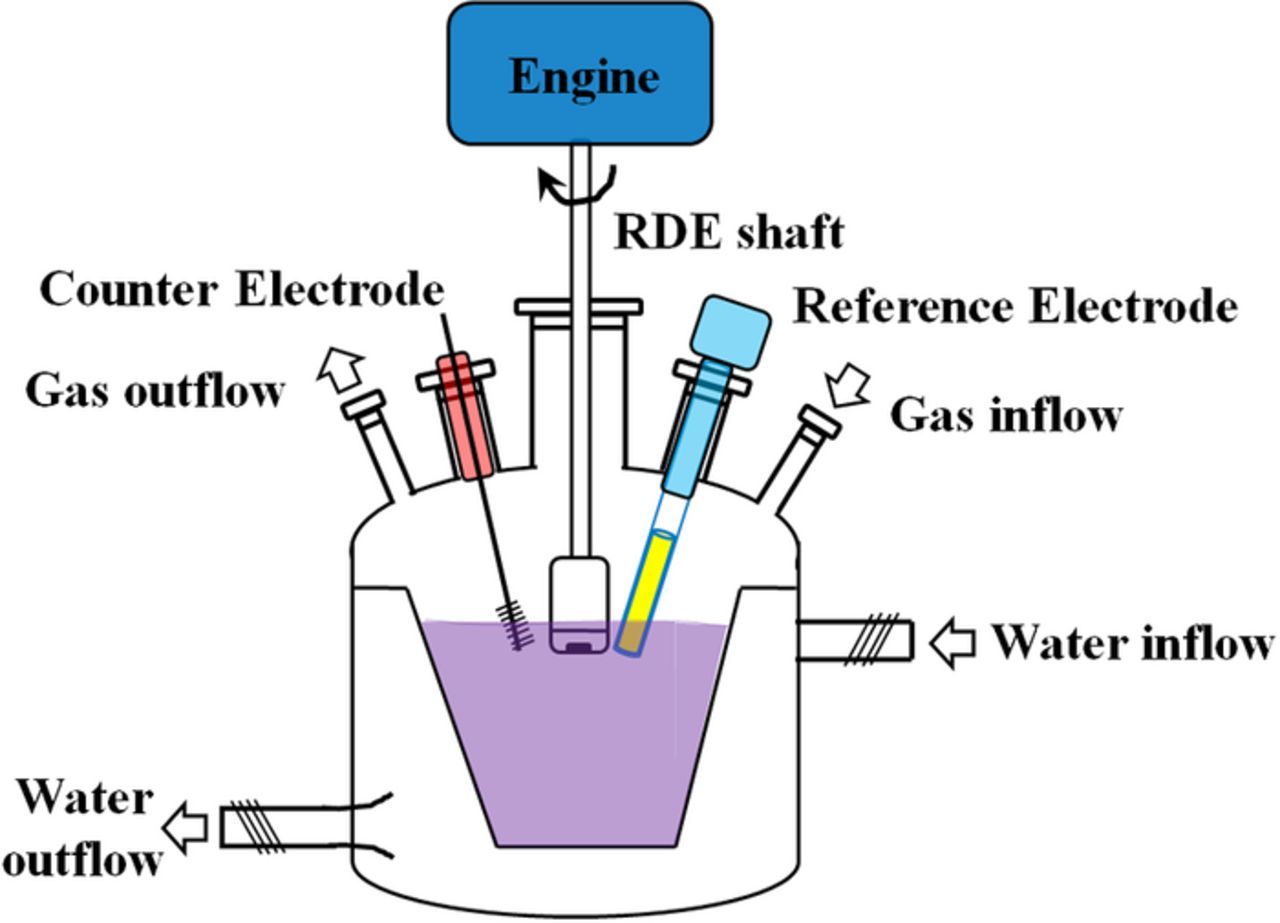
Figure 11. Schematic of a typical water-jacketed RDE cell.
The typical result from an RDE experiment is a linear sweep voltammogram, shown in Figure 12a. Note that there is no peak current, as in CV, but a steady-state, limiting current. The Levich equation relates this limiting current at a RDE to rotation speed and the physical properties of the system, as shown in Eq. 8:
![Equation ([8])](https://content.cld.iop.org/journals/1945-7111/165/5/A970/revision1/d0008.gif)
where n is the number of electrons transferred, D0 is reactant species diffusivity, ω is rotation rate, v* is kinematic viscosity, and Co is the reactant species at the surface, depending on electrode polarity.143 The limiting current obtained via RDE is typically much larger than the peak current found in stationary electrode CV due to the convective flux to the RDE surface. Additionally, reversing the polarity of the RDE will not result in a comparable reverse current because redox products are continually swept away from the surface. Figure 12b is an example set of data resultant from a Levich analysis for a system with facile kinetics and exhibiting convection-controlled current:
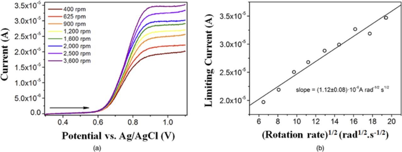
Figure 12. Levich analysis of kinetic behavior for a polymer-based RFB (a) linear voltammograms at varying RDE rotation rates and (b) Levich plot showing linear dependence of limiting current on square root of rotation rate.164
When the Levich plot is linear over a large range of rotation rates (e.g. 50–10000 rpm), the reaction can be assumed as a single, rapid transfer of n electrons with a relatively large rate constant. Assuming one knows two of the variables in the Levich equation, the third property can be found (e.g., knowing n and v* allows one to determine D0 from the slope). With this formulation, RDE is frequently paired with stationary CV since they can provide complementary results.
There are systems that will exhibit sluggish kinetics and mass transport limitation in a RDE setup. Because mass transport is facilitated in an RDE, these instances arise when electrode properties may not support fast kinetics or the reaction itself may not be kinetically fast, bringing the kinetic rate down to one that is comparable to that of mass transport (as opposed to the scenario that is described by the Levich equation, above). When this is the case, a modification to the Levich equation is employed; in its most-used form, the reciprocal of measured current is comprised of a reciprocal kinetic current and a mass-transport-dominated component to the current. This behavior is described by the Koutecky-Levich equation, shown in Eq. 9.143
![Equation ([9])](https://content.cld.iop.org/journals/1945-7111/165/5/A970/revision1/d0009.gif)
In this analysis, similar linear sweeps are performed for a RDE with varying rotation rates, as shown in Fig. 13a below. The reciprocal steady-state currents at particular overpotentials are plotted against ω− 1/2, shown in Fig. 13b. A major benefit to this style of analysis is that one can calculate the kinetic current (and a resultant kinetic rate constant) from the y-intercept of a Koutecky-Levich plot while also verifying or identifying n or D0, based on the slope of the figure.
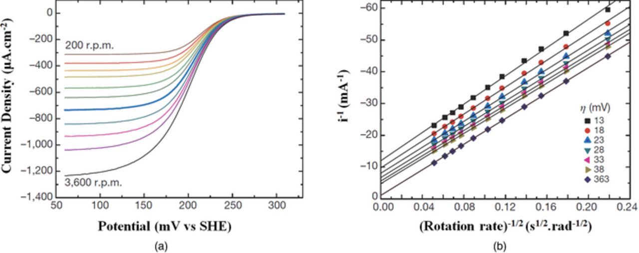
Figure 13. Koutecky-Levich analysis of kinetic current for an organic molecule-based RFB (a) linear voltammogram and (b) resultant Koutecky-Levich plot with y-intercept equal to reciprocal kinetic current at varying electrode overpotential.25
One complication that arises from RDE analysis is that the kinetic information extracted with this method is highly dependent on the preparation and form of the electrode.165 Indeed, the kinetic rate constant can vary tremendously, not only based on an electrode's native morphology and behavior, but also as a result of preparing or modifying the electrode for RDE analysis.17,150 Glassy carbon is commonly the base electrode material employed in RDE analysis, but electrochemical behavior on glassy carbon isn't necessarily representative of in-situ kinetic behavior of a 3D electrode surface. Attempts are made to circumvent this by preparing RDE electrodes that incorporate RFB electrode material, but this must be pulverized and mixed with a binder, changing material properties. In whatever form, the electrode must be capable of withstanding a high rotational speed (e.g. up to 3000 rpm). Inherent in a Koutecky-Levich assessment of any transport-related property (number of electrons, diffusivity, or viscosity) is that all other parameters are constant with rotation rate and overpotential, as well as homogenous over the entire RDE surface. Without all other parameters being constant, calculation of that parameter will be erroneous, leading to significant over- or underprediction of a property.135
Current interruption (CI)
Current interruption (CI) is an in-situ technique used to relate the transient voltage response from a current interruption event to cell parameters, most commonly ohmic resistance.166 The ratio of the change in voltage to the current that was applied before the interruption event yields the ohmic resistance ( ).167 A curve showing the voltage response to a current interruption event is show in Fig. 14. CI is more commonly applied in fuel cell literature,168,169 but can in theory be used for flow battery measurements as well.
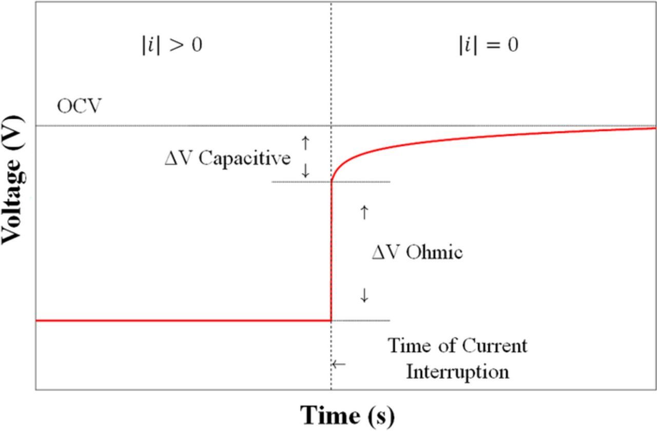
Figure 14. Current Interruption technique.
While most studies use CI to measure total internal resistance, analysis of the voltage transient has also been used to study kinetics. This method was used in conjunction with electrochemical impedance spectroscopy (EIS) in PEM fuel cells research170,171 for model validation. Here Tafel slopes were determined from voltage transient data to calculate exchange current.
Current interruption has several stipulations to consider when used. As Lagergen et al.172 discussed, accurate iR measurements are contingent upon delay time. The voltage response is governed by the imposed current as well as the capacitive current that is built up at the electrode surface. The ohmic drop occurs almost instantaneously while the capacitive current discharges more slowly. Hence, getting an accurate ohmic resistance measurement with this method depends on having an understanding of the time scale for the voltage relaxation (typically on the order of 10−6 s167,170 or 10−9 s).168 Srivanasan et al.173 reported a mathematical model which demonstrates the effect of incorporating exchange current (i0) and double layer capacitance (CDL) into estimating voltage relaxation time constant. CI has also been used on the stack level for fuel cell research as Mennola et al.174 reported. Here, an improved approach was used to determine the iR drop, which helped to compensate for error in the voltage transient sampling. In practice, the ease of interpreting internal resistance from EIS renders CI absent from most flow battery literature and as a result, this technique is not commonly used in the study of redox flow batteries.
Electrochemical impedance spectroscopy (EIS)
The application of EIS requires a small voltage/current perturbation signal of known amplitude and frequency to the cell, forcing the cell to deviate from equilibrium by a very small magnitude. Over a spectrum of frequency, the amplitude and phase of the resultant, measured signal is recorded.
In practice, there are two common experimental techniques used for conducting an EIS experiment, depending on whether current (galvao-EIS or GEIS) or voltage (potentiostatic EIS or PEIS) is controlled. In PEIS, the full bandwidth supplied by the frequency response analyzer of the potentiostat is often utilized. GEIS is predominantly utilized for linear systems (systems with facile kinetics and negligible capacitive current); as a result, for RFBs, PEIS technique is more common. A detailed review of AC impedance technique is available in another review paper.175
Impedance spectra can be plotted in the form of a Bode diagram (impedance magnitude and phase angle as a function of frequency) and/or the more common Nyquist diagram (the imaginary component of impedance versus the real part at each frequency). A typical Nyquist plot for an RFB is shown in Fig. 15, with the ohmic (series and distributed), charge-transfer, and finite diffusion resistances (overpotentials) denoted.
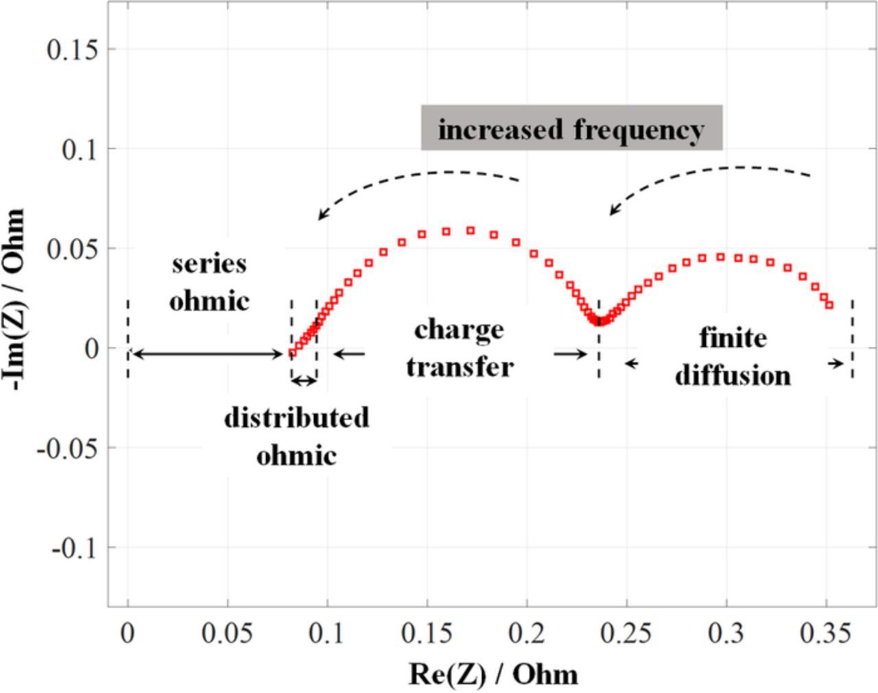
Figure 15. Typical impedance spectrum.
To obtain quantitative values from a Nyquist plot, the impedance results can be fitted by an equivalent circuit, often the Randles circuit or a close variant.176 It is common to replace the capacitor element in the Randles circuit with a constant phase element (CPE) in order to account for non-ideal capacitive behavior of the electrodes.176
In Fig. 16, Rsol represents ohmic impedance (comprised of ion-exchange membrane resistance, contact resistances, solution resistance and electrode resistance), Rct represents charge transfer resistance across the electrode-electrolyte interface, and W represents the Warburg element for finite diffusion. Rsol typically occurs at very high frequency (5–30 kHz) while the Warburg element manifests itself in a Nyquist plot by a 45-degree line in the low frequency region. It is also important to note that the value of the constant phase element can be converted to the value of double layer capacitance across the electrode-electrolyte interface.137 Thus, if applied correctly, EIS can yield quantitative insight into all overpotentials observed in a RFB.125
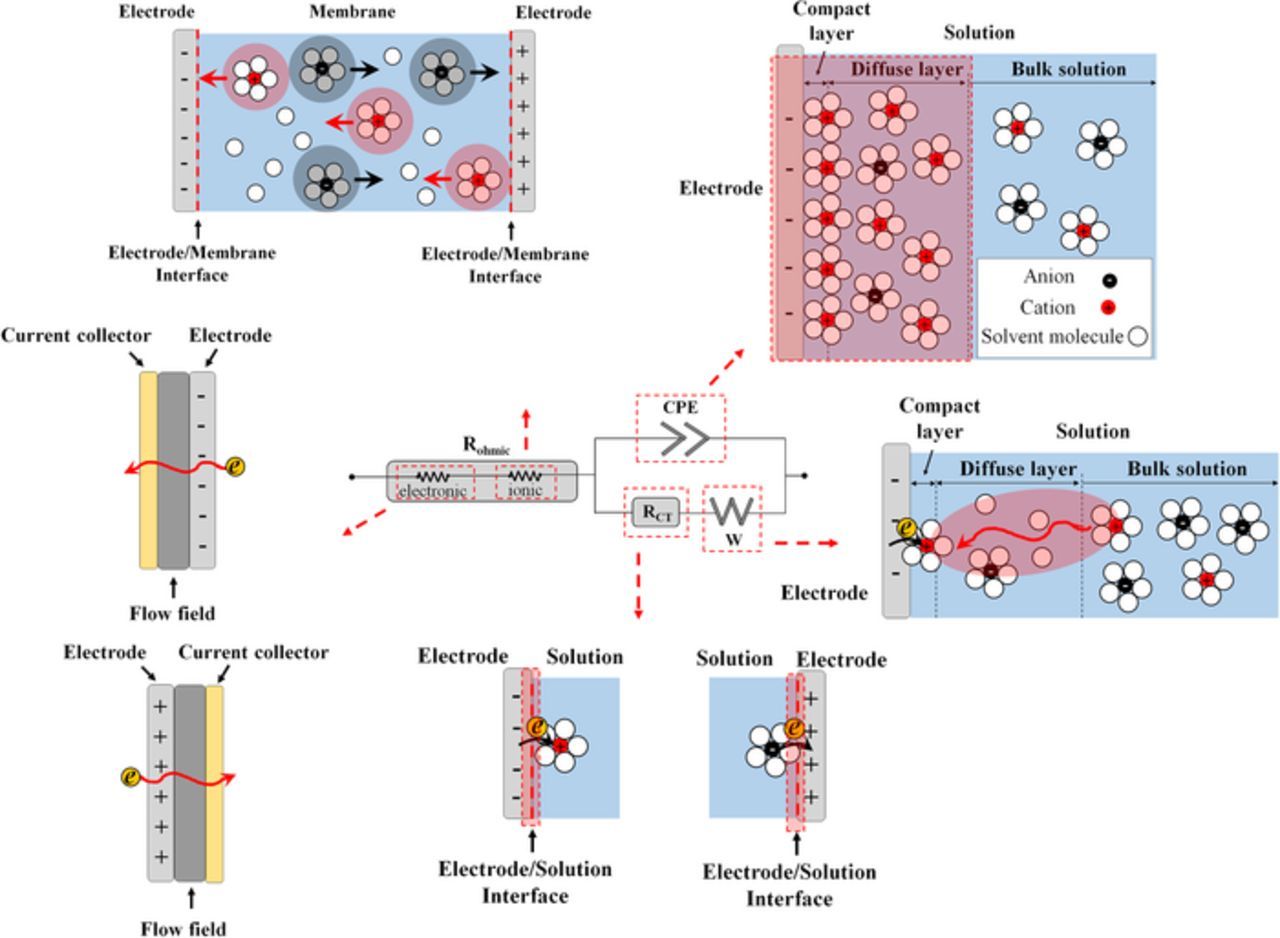
Figure 16. Schematic of Randles equivalent circuit model and elements.
The main advantage of the EIS technique is to resolve various sources of polarization for an operating cell under different conditions. If one obtains impedance spectra at several currents, these resistances can be integrated as a function of current to obtain the total overpotential due to each process within the system, allowing for identification of the most rate-limiting process/component for a particular cell design and electrolyte composition. For example, charge transfer resistance is defined by the following equation.177
![Equation ([10])](https://content.cld.iop.org/journals/1945-7111/165/5/A970/revision1/d0010.gif)
As is clear from Eq. 10, integrating the charge transfer resistance as a function of current will result in the charge-transfer overpotential. A similar approach can be applied for ohmic and mass transport impedance to obtain the overpotentials associated with each category. Further details regarding theoretical modeling of an EIS spectrum are available elsewhere.137,178 An impedance-resolved polarization curve is shown in Fig. 17.
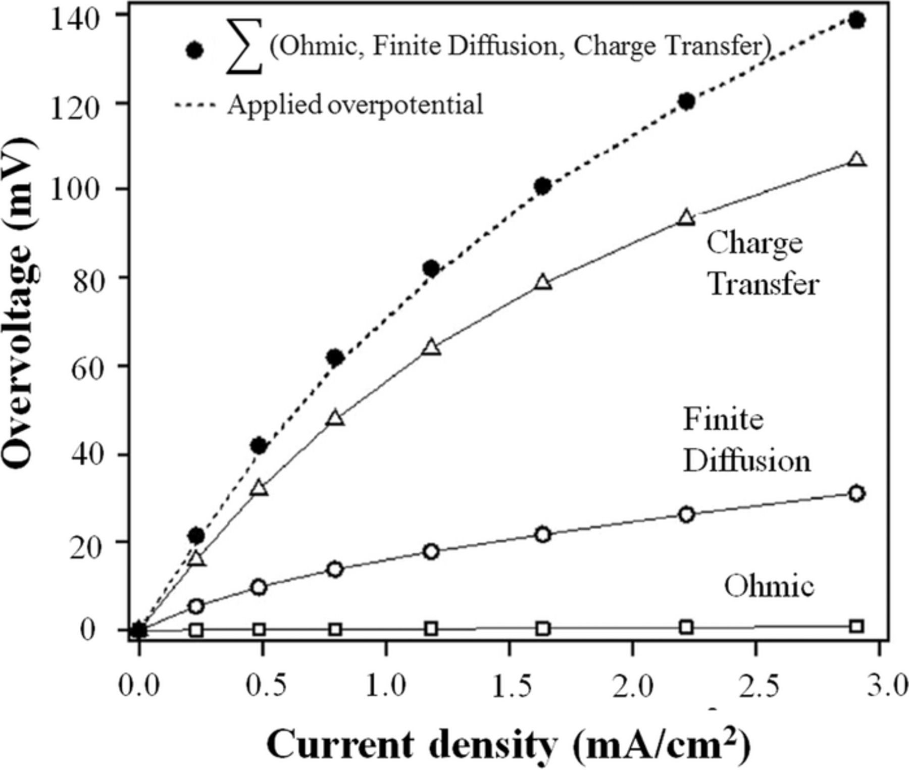
Figure 17. Overpotentials associated with the ohmic, charge transfer and finite diffusion process for an RFB (Ref. 137).
While EIS provides relatively detailed information, it has major limitations. First, the impedance spectrum can be distorted for high concentration systems (as in RFBs) in the low frequency regimes by commonly-used pumps (e.g. peristaltic, diaphragm). The pulsing nature of these pumps necessitates extra equipment to stabilize impedance responses at low frequency.179 Resolving this issue can be done with constant flow syringe pumps or having a pressurized intermediate reservoir in which pump pulses are dampened by a gas headspace. Alternatively, relatively low concentration of electroactive species (ca. 0.1–0.5 M) can alleviate low frequency distortion.
Due to the previously-mentioned distortion at low frequency, EIS is frequently used to study ohmic and charge-transfer kinetics overpotentials.125,137,180,181 Even at frequencies avoiding pump-based distortion, some obstacles must be overcome to obtain reliable EIS results. Investigators must find a suitable reference electrode that is physically compatible with the electrochemical cell, while also being electrochemically stable. Interpretation of impedance spectra requires knowledge of active species concentrations, which may change as a result of crossover in full-cell measurements. Furthermore, interpretation of impedance spectra is not always straightforward, which can lead to incorrect conclusions regarding data.137 EIS is also a cell-averaged method, thus distributions in current and potential are not easily quantified. EIS has been applied to a variety of chemistries, including all-vanadium,125,137 aqueous organic,26 hybrid air-vanadium,138 non-aqueous vanadium,182 and iron slurry,183 among others. Reference 184 is a comprehensive text for more detailed information about EIS.
UV-Vis spectroscopy
Ultraviolet–visible spectroscopy (UV-Vis) is utilized to obtain quantitative information regarding the concentration of the ionic species within an electrolyte if the electrolyte has discernable signal variation between dissolved ions. UV-Vis is a type of absorption spectroscopy in the ultraviolet-visible spectral region. This technique requires a light source in the visible and adjacent ranges (near ultraviolet-visible) and a spectrometer. UV-Vis operates based on the principle that non-bonding electrons can absorb energy in the form of ultraviolet (10–380 nm) or visible (380–780 nm) light; such absorption excites these electrons to higher anti-bonding molecular orbitals and is correlated to the absorbing wavelength (easily-excited electrons are related to longer wavelength).
The light source and spectrometer can be integrated into a single device or can be separate devices based on the particular application of interest. Figure 18 is a schematic of a system where the detector (spectrometer) and light sources are separate devices, usually separated by a fiber optic light guide; integrated source-spectrometer devices are typically built as a single unit where the sample is inserted into the light path. An advantage of the separate source-spectrometer arrangement in Fig. 18 is that the sample chamber can be constructed to allow for liquid flow through it, enabling real-time UV-vis spectroscopy on a RFB electrolyte.
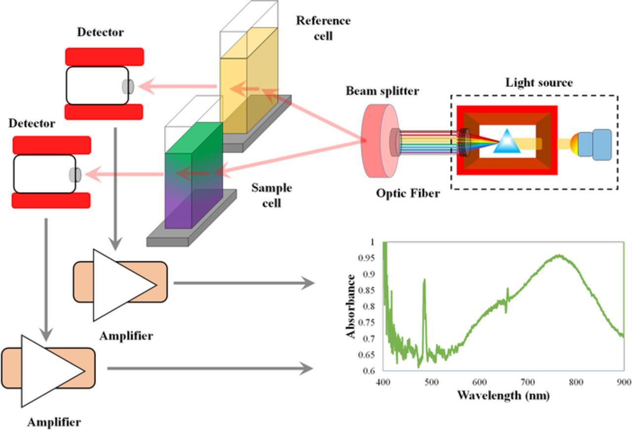
Figure 18. Schematic of UV-Vis setup.
UV-Vis spectroscopy can be used to quantitatively determine concentrations in a solution or electrolyte. This technique requires samples to be vividly colored in order to guarantee strong absorbance spectra. As a result, transition metal ions and highly conjugated organic compounds in solution are detectable using this technique. To determine the concentration of a particular species within the solution, the intensity of light transmitted through a solution can be measured relative to a clear medium (e.g. measuring light intensity for a solution of vanadium relative to the intensity through the supporting electrolyte without vanadium), as described in Eq. 11.
![Equation ([11])](https://content.cld.iop.org/journals/1945-7111/165/5/A970/revision1/d0011.gif)
In Eq. 11, I is the measured light intensity of the solute-bearing solution, I0 is the baseline intensity of a solution without the solute of interest, l is the path length, ς is the cross-section area, N is the number density of the absorbing molecules. The absorbance ( ) is defined as:
![Equation ([12])](https://content.cld.iop.org/journals/1945-7111/165/5/A970/revision1/A970equ1.jpeg)
Beer's law is utilized in terms of molar concentration (cm) and molar absorptivity (am) in order to obtain the absorbance (A*) in Eq. 13.
![Equation ([13])](https://content.cld.iop.org/journals/1945-7111/165/5/A970/revision1/A970equ2.jpeg)
If multiple absorbing solutes exist within the solution, it is assumed that the total absorbance is the linear combination of them. As a result, in practical applications, usually the absorbance of spectra at two different wavelengths (i.e. λ1 and λ2) is obtained and the following set of equations is solved simultaneously in order to obtain the concentrations (cα and cβ).
![Equation ([14])](https://content.cld.iop.org/journals/1945-7111/165/5/A970/revision1/A970equ3.jpeg)
![Equation ([15])](https://content.cld.iop.org/journals/1945-7111/165/5/A970/revision1/A970equ4.jpeg)
A typical absorbance spectrum used for the calculations of Eqs. 14 and 15 has been shown in Fig. 19. In this case, absorbance maxima occurred at both ∼560 nm and ∼855 nm, corresponding to λ1 and λ2, respectively.
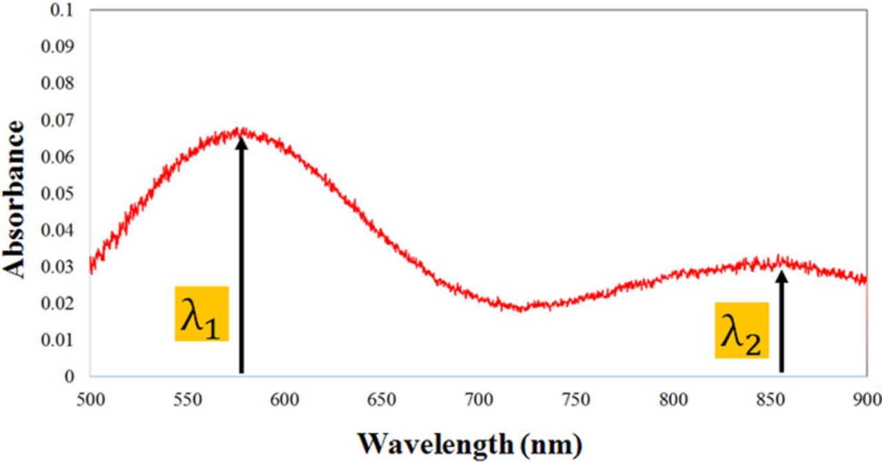
Figure 19. The absorbance for the solution of two solutes.
The UV-Vis technique provides a simple, robust, quantitative method for determining concentrations. The absorbance spectrum shown in Fig. 19 can be measured ex-situ or in-situ. For VRFBs, this technique was originally used to determine the electrolyte SoC since all four oxidation states of vanadium absorb at separate wavelengths.185 More recently, comprehensive mathematical models have been developed based on absorbance spectra in order to determine the SoC for VRFBs.186–188
The UV-Vis spectroscopic method can also be used to measure crossover by coupling with a permeability cell.102,114,189 This approach targets concentration-gradient induced crossover in which a solution containing electroactive species (enriched side) is circulated on one side of a membrane while the other side is deficient of electroactive species. This technique to assess crossover has been successfully applied for all-vanadium RFBs and vanadium-air hybrid RFBs as summarized in Table III. The permeability cell has also widely been used to quantify the water transport through various types of nano-porous membranes for membrane-based water desalination.190–193
Table III. Crossover research summary in the literature.
| RFB Type | Species type | Ref. |
|---|---|---|
| All-Vanadium | V(II) | E. Wiedemann et al.194 |
| V(III) | ||
| V(IV) | ||
| V(V) | ||
| All-Vanadium | V(III) | X. Luo et al.195 |
| V(IV) | ||
| V(V) | ||
| All-Vanadium | V(II) | C. Sun et al.196 |
| V(III) | ||
| V(IV) | ||
| V(V) | ||
| All-Vanadium | V(II) | Q. Luo et al.197 |
| V(III) | ||
| V(IV) | ||
| V(V) | ||
| All-Vanadium | V(IV) | J. S. Lawton et al.198,199 |
| All-Vanadium | V(IV) | W. Xie et al.200 |
| Vanadium-Air | V(II) | J. G. Austing et al.201 |
| V(III) | ||
| All-Vanadium | V(II) | Y. Ashraf Gandomi et al.102,114 |
| V(III) | ||
| V(IV) | ||
| V(V) |
Although UV-Vis spectroscopy is a robust technique, it requires a customized set-up if the required measurements are to be done in-situ. Also, the major requirement for determining concentrations using this technique is a linear dependence of absorption on concentration. This requirement is not guaranteed for all solutions and RFB electrolytes, thus calibrations for all compositions are necessary.
Potential distribution
Potential distribution is a distributed diagnostic technique that can be applied to obtain the potential of half-cells and bipolar plates in a multi-cell stack. This technique can also be applied to obtain in-plane and through-plane solid-phase and liquid-phase potential distributions. This technique requires the installation of a stable reference electrode.
Previous studies on polymer electrolyte membrane fuel cells (PEFC) have discussed the installation of a reference electrode that is stable, yet fits within the tightly-layered structure of a PEFC or RFB.202,203 The most common reference electrode configurations are sandwich-type and edge-type. In the sandwich-type, a thin conductive wire is inserted between two membranes.115,204,205 In the edge-type configuration, the reference electrode is attached to a region of the ion-exchange membrane outside the active area between the two electrodes.206,207 It is important to minimize the distance between the reference electrode and the working electrode when placing the reference electrode in order to minimize iR overpotential. The simplest measurement afforded by reference electrode inclusion is measurement of each half-cell potential during RFB operation; an insight that cannot be obtained without a reference electrode. If the more complex potential distribution measurement is needed, special cell design and configuration are required.
Ng et al. designed a cell with multiple working electrodes using a copper mesh (Fig. 20a) which was implemented in the in-plane configuration across the electrode thickness of an operating lithium-ion battery.208 Hess et al. measured the electrolyte potential distribution through the thickness of a PEFC electrode.209 The same group measured the electrode and electrolyte potential distribution (Fig. 20b) through the negative electrode of an electrochemical double layer capacitance for an aqueous sodium hybrid battery during charge and discharge.210,211 Potential distribution diagnostics have also been implemented for microfluidic fuel cell architecture,212 a PEFC equipped with a non-precious catalyst,213 and flowable electrodes.214 Recently, the potential distribution technique was applied to an all-vanadium redox flow battery.115,215 Ashraf Gandomi et al. inserted micro-probes into the layers of a multi-layer electrode (Fig. 20c) in an operating all-vanadium redox flow battery to measure the solid-phase, through-plane potential distribution between the flow fields and the membrane.115
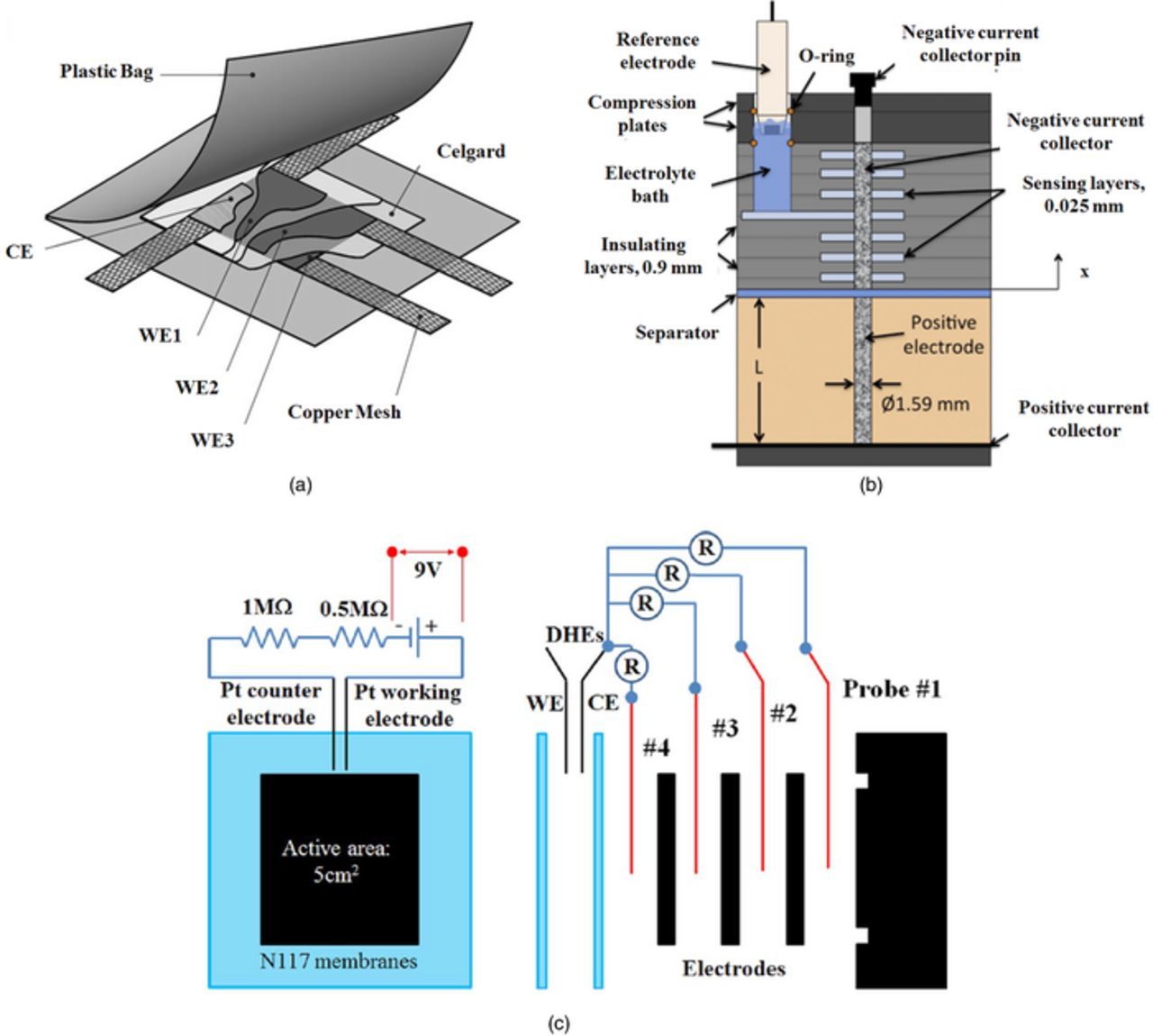
Figure 20. Different potential distribution setups, (a) in-plane potential distribution diagnostics using copper mesh implemented to a lithium-ion battery,208 (b) Through-plane solid- and liquid-phase potential distribtion diagnostics applied to an aqueous sodium hybrid battery,211 (c) Through-plane solid-phase potential distribution diagnostics applied to the multiple layers of electrode stack for a VRFB.115
Potential distribution allows in-situ assessment of both the solid-phase and electrolyte-phase potential distribution. Information can be gained regarding electroactive species consumption between the flow fields and the membrane (related to electrode utilization), as well as between the inlet and the outlet, regardless of flow field geometry. In all of these, incorporating a stable reference electrode can be challenging with many RFB systems because sometimes-significant modifications to the design must be made. Particular care must be paid to ensuring there is no leakage around where probes or wires cross gaskets, the environment around the reference electrode is compositionally stable, and distinction between solid- and liquid-phase potential is accurately made. With these precautions addressed, potential distribution measurement can provide tremendous insight suitable for inclusion in multi-dimensional models.
Nuclear magnetic resonance (NMR)
Nuclear magnetic resonance (NMR) spectroscopy is primarily used to observe the migration of cations or anions. NMR spectroscopy exploits the magnetic properties of atomic nuclei and is applicable to a wide range of samples, including solutions and solids. For this spectroscopic measurement, a sample is placed in a magnetic field and NMR-active nuclei absorb electromagnetic radiation at a frequency characteristic of the isotope. The strength of the magnetic field affects the resonant frequency, energy of absorption, and the intensity of the signal. A commonly-applied magnetic field is 21 Tesla (900 MHz). A more comprehensive description regarding NMR spectroscopy is available in Refs. 216,217.
Upon excitation of the sample with a radio frequency pulse, a nuclear magnetic resonance response (time-domain) is obtained followed by a Fourier transform to extract the frequency-domain spectrum. A schematic of an NMR spectroscopic setup is shown in Fig. 21.
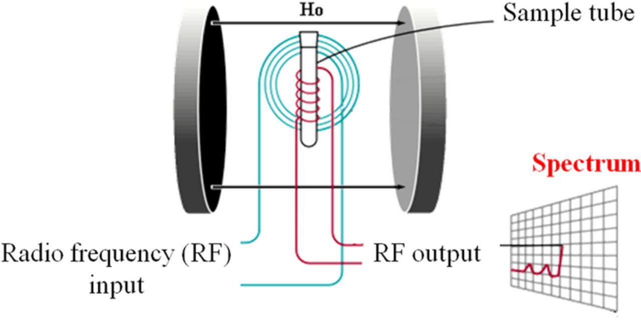
Figure 21. NMR setup (Figure adopted from the Ref. 218).
An NMR spectrum is a plot of the radio frequency applied against absorption. The frequency of a signal is known as its chemical shift. Chemical shift is defined in Eq. 16.
![Equation ([16])](https://content.cld.iop.org/journals/1945-7111/165/5/A970/revision1/d0016.gif)
In Eq. 16, fs is the frequency of the signal, fref is the frequency of the reference signal and fsp is the spectrometer frequency. The reference frequency is defined at 0 ppm of the material of interest. A typical NMR spectrum is shown in Fig. 22.
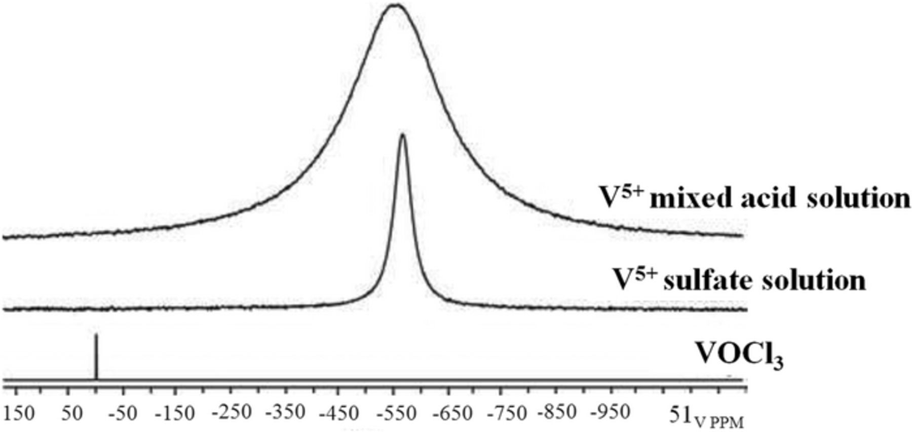
Figure 22. Typical NMR spectra (from Ref. 72).
NMR spectroscopy has been widely used in RFBs and PEFCs for studies on solution and separators to identify and quantify the species of interest.219–221 NMR has also been applied to obtain the ionic diffusivities in other fuel cell types (i.e. methanol diffusion in PEFCs has been studied with NMR).221 The effect of supporting electrolytes for aqueous solutions has also been studied with NMR.222 NMR spectroscopy has also been used to study solubility in aqueous solutions.72,223 Also, assessment of species diffusion within the bulk portion of an ion-exchange membranes has been conducted using NMR.224 Although very useful, NMR is a relatively expensive technique, thus it is not widely reported in the RFB literature. The main limitation of NMR spectroscopy is relatively less sensitivity compared to mass spectroscopy diagnostics.225 This limitation necessitates much larger samples to be used for analysis. Also, among the various types of nuclides detectable by NMR, proton (1H) is the most widely used one in the literature due to exhibiting high sensitivity.225 Also, as a result of relatively low sensitivity, signal averaging is required for almost all measurements in order to achieve an acceptable signal-to-noise level and this, complicates the analysis of NMR data for most cases.225
Ionic and electronic conductivity measurement
Conductivity measurements can be performed in-situ or ex-situ. Usually, in-situ conductivity measurements include combined effects of both ionic and electronic conductivity of the series-connected components in the cell. As a result, ex-situ conductivity measurements are of great importance because they enable the study of conductivity at the individual component level. Additionally, ex-situ conductivity measurement can be done on relatively small samples and with greater rapidity than those done in-situ. Conductivity measurements can be done to assess electronic, thermal, and ionic conductivity. Electronic conductivity measurement is usually straight forward and operates on the principle of Ohm's law for a conductor. The ionic conductivity is usually measured to assess the conductivity of the solution (electrolyte) as well as the conductivity of the ion-exchange membrane (separator). In order to measure the conductivity of a liquid electrolyte, an external conductivity meter is usually used. Skyllas-Kazacos et al. measured the conductivity of vanadium electrolyte as a function of state of charge (SoC) and of supersaturated vanadium solutions.222,226 The ionic conductivity of these solutions is of interest since it comprises a significant share of the total internal resistance in most RFBs. However, little optimization of solution conductivity has been done to date.
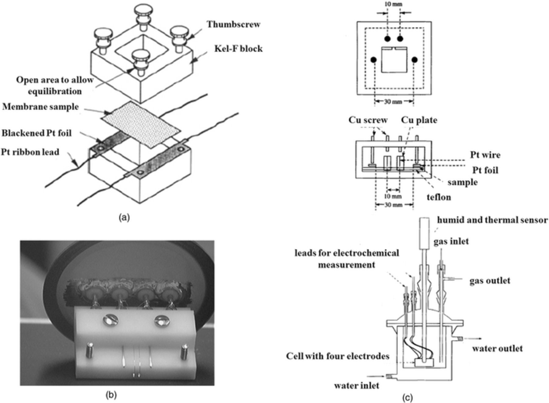
The ionic conductivity of separators is usually measured using the four-electrode AC impedance technique. T. A. Zawodzinski et al.219 measured the conductivity of partially-hydrated Nafion membranes using such a conductivity cell, as shown in Fig. 23a. M. Doyle et al.227 measured the conductivity of perfluorinated ionomers as a function of non-aqueous solvent properties using the conductivity cell shown in Fig. 23b. Y. Sone et al.228 measured the proton conductivity of Nafion 117 using a four-electrode cell (Fig. 23c). In this measurement, two platinum foil electrodes (3 cm apart) were used to conduct current and two platinum needles (1 cm apart) were used to measure the potential drop.228 In all of these four-point cell measurements, similar principles are employed. Calculating the conductivity (σ) is performed according to Eq. 17.
![Equation ([17])](https://content.cld.iop.org/journals/1945-7111/165/5/A970/revision1/d0017.gif)
where Ls is the distance between voltage probes, Rs is the resistance of the medium (e.g. a membrane), and Ss is the cross-sectional area of the medium. The resistance, Rs, is typically obtained by measuring the high frequency resistance between the voltage probes.
The conductivity cell has also widely been used to study the ionic conductivity of different types of ion-exchange membranes exposed to various bathing electrolytes (aqueous and non-aqueous)229–234 and has been implemented to assess the degradation of membranes during long-term cycling.235 The ionic conductivity measurement using a four-electrode cell, although facile and rapid, requires care since this test is conducted ex-situ under conditions likely very dissimilar from those experienced in the cell. It is critical to guarantee the species uptake states are similar to the in-situ operational conditions. The in-plane conductivity of the ion-exchange membrane is typically obtained over a range of operating conditions in order to quantify the optimum conditions to achieve the highest ionic conductivity.233,236 Figures 24 and 25 show examples of measuring in-plane ionic conductivity for an ion-exchange membrane using a conductivity cell and ionic conductivity of solution using an external conductivity meter.
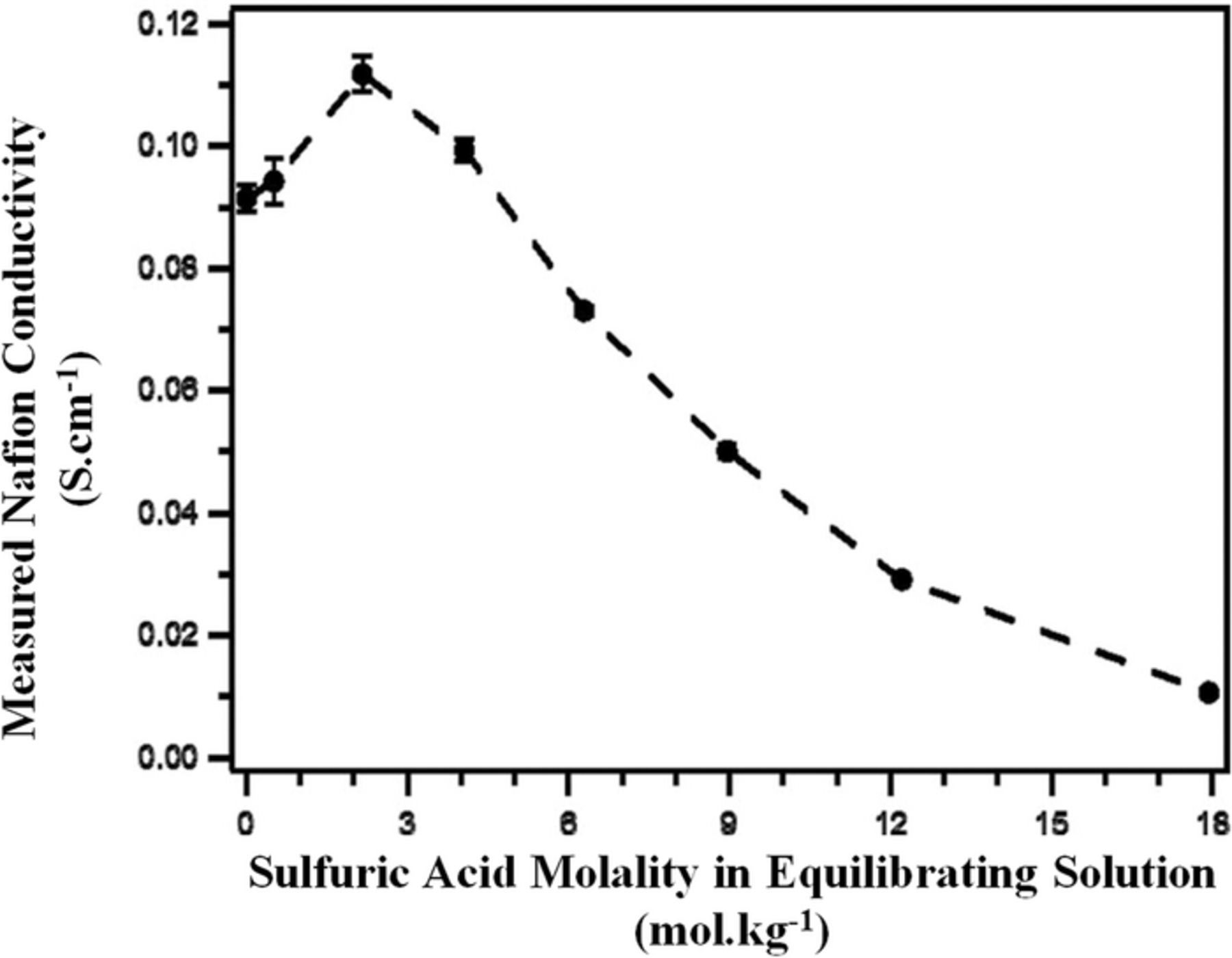
Figure 24. Measured membrane conductivity as a function of sulfuric acid concentration in the electrolyte (Ref. 233).
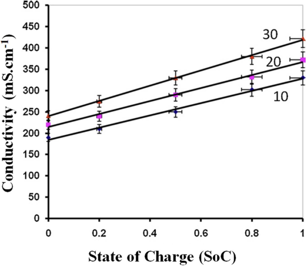
Figure 25. Measured conductivity of negative electrolyte (V(II)/V(III)) as a function of SoC at various temperatures (10, 20, and 30°C) for all-vanadium redox flow batteries using external conductivity meter (Ref. 226).
It is important to note that the conductivity measured using a conductivity cell enables the measurement of in-plane conductivity for the membranes. Depending on the morphology of the membranes and the degree of reinforcement, the properties of the membranes might exhibit inhomogeneity and therefore, the through-plane conductivity is not the same as in-plane conductivity. The through-plane conductivity is usually measured using electrochemical impedance spectroscopy. Also, it is important to note that in comparison of in-plane and through-plane conductivity assessment, the electrolyte in contact with the membrane is also critical. The in-plane conductivity measurement usually is performed in ambient environment; however, the through-plane measurement is conducted in real cell conditions in which the electrolyte-electrode-membrane boundary is the boundary conditions for the membrane for equilibrium and non-equilibrium conditions.
In addition, it is important to mention that according to Fig. 23, it is critical to precisely measure the thickness and the width of the samples being used in conductivity cell. This measurement is cumbersome since the ionic uptake, elongation and stress-strain characteristics of the samples are strongly being affected by the soaking solution. Additionally, the applied pressure within the conductivity cells are not necessarily accurately controlled, which can also affect the measurement if not taken into account.
Electron spin resonance (EPR) spectroscopy
Undesired transport of ionic species and water (crossover) is a behavior of interest in redox flow batteries, thus multiple techniques are employed to understand this phenomenon. For VRFBs, crossover is merely a form of self-discharge. However, it is of greater concern for Fe/Cr and H2/Br flow batteries, as crossover may result in irreversible losses. Another tool employed to characterize membrane behavior is electron spin resonance spectroscopy, also called electron paramagnetic resonance (EPR) spectroscopy.237 This technique measures rotational diffusion for several materials, including organic free radicals and transition metals. When applied to VRFBs, EPR is limited, in that it only directly detects VO2+ and V2+. However, these two species have been shown to infiltrate and accumulate in Nafion unlike VO2+ and V3+.224 Thus, the directly-detectable species are most relevant for uptake and crossover studies. EPR also frequently includes the addition of spin probes – small molecules with stable free radicals that can elucidate fine features related to solvent motion and viscosity in the pores of a hydrated membrane. Such observations aid in understanding the environment inside ion exchange membranes. The presence of the probes can be used to report on the potential transport of species not directly detectable with EPR, including V3+ and VO2+.238 Consequently, EPR is used to quantify the uptake and transport of vanadium in VRFBs. This insight informs better understanding of water, proton, and vanadium crossover since all of these species interact in bulk solution as well as in most cation exchange membranes.239 It is noted here that EPR studies are not limited to Nafion; recent work has shown that EPR has been used in assessing the vanadium uptake in sulfonated Diels-Alder poly(phenylene) membranes-a hydrocarbon-based alternative to Nafion in VRFBs.199 Via EPR experiments, VO2+ uptake has been quantified and the results agree with studies that did not utilize EPR.240
Membrane properties of interest, including permeability and partitioning coefficient, have been investigated with EPR, as well. These experiments are accomplished typically by soaking membranes in an electrolyte representative of conditions in a VRFB and then placing the samples in an EPR spectrometer, similar to four-point conductivity probe measurements. In addition to observations of the environment inside ion exchange membranes, modified EPR experiments have been executed to measure vanadium crossover in permeation cells.198 In this work, the spectrometer was modified to measure VO2+ concentration in real time for the permeate side of the permeation cell, akin to the more common UV-Vis spectroscopy experiments described in UV-Vis spectroscopy section.
The insights gained by EPR appear relatively infrequently in the literature since the equipment required to do this measurement is expensive and the technique cannot directly detect all species. However, detailed studies of motion in membranes can be accomplished via EPR, thus it is useful and complimentary to the more common NMR.
Flow visualization techniques
Visualization techniques in RFBs identify electrolyte flow distribution and have been conducted via optical and thermal methods. Optical visualization of RFB flow distributions is an area that has been scarcely explored due to system and component limitations. Further details regarding the optically transparent cells for flow visualization is available in another reference.241 The primary obstacle is the opacity of the porous electrode and structural materials. This opacity, combined with the three dimensional and porous nature of the electrode, hinders attempts to use standard light-based methods such as shadowgraphs, schlieren photography, and interferometry, all of which require light to penetrate throughout the entire flow domain. Additionally, fluorescent techniques involving the addition of dyes to measure concentrations can merely give a two-dimensional result on the electrode surface. While various particle tracing methods such as Positron Emission Tomography (PET) may eventually become a solution, light-based tracing techniques suffer from the same issues as most optical methods. Those involving X-ray or computed tomography do not yet have the necessary spatial or temporal resolution for such a task within the electrode, and may not be even suitable for characterizing channel and manifold flow depending on the geometry. Some of the most recent studies have reported the spatial and temporal resolution of 200 microns and 1 millisecond respectively.242
Therefore, this technique, although valuable, cannot give a complete picture of fluid transport. This lack of a suitable technique to address flow visualization in RFBs is a clear opportunity for future advancements to be made within the field.
Thermal visualization of flow distribution is a relatively new ex-situ technique that employs a Reynolds analogy in order to directly visualize electrolyte flow within the electrode.243 The method gives useful insight into the transport mechanisms and flow mixing and distribution within the electrodes by correlating mass transport with thermal transport. This visualization technique uses a half cell, but replaces the membrane with a thin, heat sensitive liquid crystal sheet (LCS) in direct contact with the electrode. A clear viewing plate is placed on top of the LCS, followed by an endplate with a viewing window for compression. Chilled water is pumped through the cell before testing to ensure that the electrode attains thermal equilibrium; heated water is then pumped through the cell. The heated water induces a color change in the LCS. Since heat transfer and mixing is highest at locations with high convective flow, the color gradients that develop represent a direct visualization of the electrolyte flow through the electrode. This method provides an important qualitative confirmation of the relationship between current distribution measurements and convective flow through the electrode, as well as qualitative confirmation of trends seen in electrode flow distribution modelling. An example of a thermally visualized distribution can be seen in Fig. 26 and in Sup. Material Video 1.
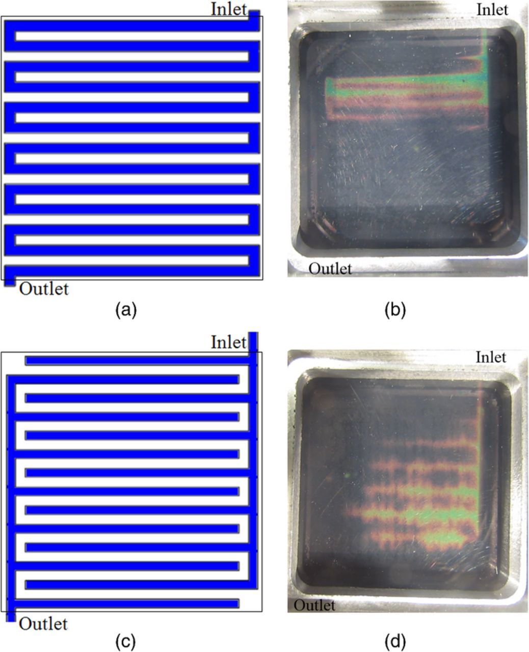
Figure 26. Cell for thermal visualization, (a) Serpentine flow field (b) Thermal visualization of flow across the electrode from serpentine flow field (c) Interdigitated flow field (b) Thermal visualization of flow across the electrode from interdigitated flow field (Ref. 106).
As a relatively new technique, thermal visualization of flow distribution has only appeared once in the literature in a study by Houser et al.106 This work uses the technique to compare the transport mechanisms in two different flow fields by validating the trends seen in a computational model as well as those produced in current distribution experiments. This technique should not be limited to such narrow applications, however, and could be used to compare changes in electrode morphology or in conjunction with techniques such as neutron imaging to further understand mass transport in RFBs.
The major limitation of this approach to visualization is that it is only capable of generating qualitative results at this point. Due to heat spread via conduction and dissipation throughout the cell, a direct correlation between fluid velocity and heat transfer has not been developed. This limits the quantitative utility of the technique for model validation and prevents it from generating usable validation data for detailed models. Additionally, due to lack of chemical compatibility, the typical acid electrolyte cannot be used, with water being the active fluid instead. This introduces a slight change in viscosity which leads to some additional error in the resulting distribution, although computational models show that this variation is minor.106
Neutron radiography (NR)
Neutron radiography (NR) or neutron imaging is a unique visualization technique with the capability to quantify water content in an optically opaque system. This tool relies on the large neutron cross sectional area of hydrogen and relative neutron-transparency of common electrochemical system materials to measure water content for pixels in the range of 10–100 μm.244 Figure 27 demonstrates X-ray and neutron cross sections for common materials used in electrochemical systems. Larger cross section results in greater attenuation of X-ray or neutron beam transmission. Attenuation is also influenced by the mass density of a component; thus, water attenuates neutrons relatively strongly while other components in an electrochemical system do not.
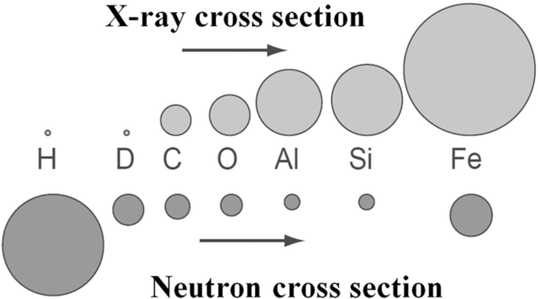
Figure 27. Neutron cross sections for common materials compared to X-ray cross sections.244
Neutron imaging is similar to X-ray radiography: a test system is placed in front a detector and hydrogen-bearing components (e.g. water) strongly attenuate neutrons that pass through the system. The detector measures neutron intensity which, with proper calibration, can be converted to water layer thickness for each detector pixel. Initial images of a dry system are collected to provide baseline neutron attenuation due to the materials used to construct a cell (e.g. graphite flow plates, aluminum endplates, graphitic electrodes, dry separator). Then, water can be introduced to the system and a range of two-phase behaviors observed as a function of operating conditions and materials ("two-phase" is noted due to the difference in attenuation between liquid- and gas-phase constituents). This technique has been used extensively at the National Institute of Standards and Technology (NIST) to measure the location, quantity, and movement of water in PEFCs245–248 and other electrochemical systems;249,250 it is noted here that both through-plane and in-plane neutron imaging experiments have been performed in PEFCs.251,252 The NR facility at NIST has been shown in Fig. 28.
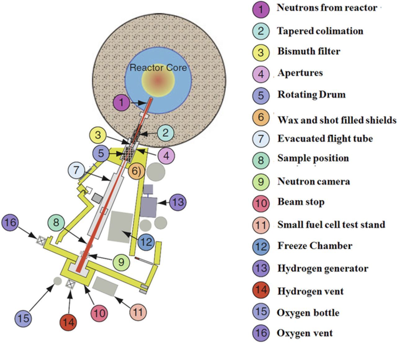
Figure 28. Schematic of the NIST neutron imaging facility.253
Many flow battery chemistries are completely liquid-phase for both half-cells, causing this technique to require special cell architecture. In general, the time required to collect sufficient neutron hits on the detector for a clear image is inversely proportional to water layer thickness. As a result, the water layer thickness cannot exceed 1–10 mm; if greater than this range, prohibitively long exposure time is required due to high neutron attenuation. For fully liquid-phase systems, relatively shallow channels, thinner electrodes, and thin graphite flow plates can yield exposure times in the 1–10 s range.254
To the authors' knowledge, neutron imaging for flow batteries has only been performed by Clement et al. at the NIST Center for Neutron Science.254 In this work, neutron imaging was used to quantify and track the gaseous products of parasitic side reactions, specifically carbon corrosion in the positive electrode of a hydrogen/vanadium battery. The hydrogen couple was used on the negative side in an effort to minimize water layer thickness and obtain reasonable exposure times (hydrogen gas, while having a large neutron cross section, is low density and contributes very little to neutron attenuation). With a H2/Pt negative electrode, most polarization in the battery was on the positive side, thus the system behaved similarly to a three-electrode cell with a combined hydrogen reference and counter electrode. The battery was charged over a range of voltages with an initial SoC of near-100%; via the neutron imaging technique, the evolution of gas bubbles could be tracked as a function of charging voltage on the positive side of the battery. Images for a series of two-minute charging steps is shown in Fig. 29 with no detectable gas evolution at 1.8 V on the positive side and extreme gas evolution at 2.3 V on the positive side. Later experiments with a mass spectrometer sampling the positive electrolyte headspace confirmed the evolution of CO2 due to carbon corrosion over this range of voltage.
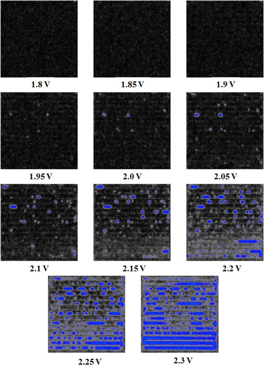
Figure 29. Colorized optical density images showing gas accumulation over 2-min charging in a hydrogen/vanadium flow battery with a serpentine flow field (V(V)/V(IV) couple). CO2 evolution was confirmed via mass spectroscopy.254
As noted, the use of neutron imaging for flow battery studies is in its fledgling stages; it has the potential to be a powerful tool, however, especially for battery systems that use at least one gas-phase couple. Even for fully-liquid batteries, neutron imaging is capable of measuring in-situ gas evolution and other two-phase phenomena with accommodations made to control water thickness. However, neutron imaging does impose some restrictions on battery geometry that limit its application; this is in addition to the fact that only a handful of facilities worldwide can perform such experiments. Also, current resolution limits are in the 5–25 μm range; this limit is increased for higher attenuation samples (e.g. liquid RFBs) and requires longer exposure times. The greatest cell geometry limitation is on water layer thickness; many RFB test cells utilize relatively thick carbon felt electrodes (1–4 mm), electrolyte channels of ∼1 mm depth, and thicker flow plates. Stack systems frequently employ thinner components, but have at least two cells in series. As a result of these architectures, the liquid phase can be thick, leading to relatively long exposure times if rapid behaviors are of interest. Additionally, some materials can be activated via neutron absorption (e.g. gold), causing them to become radioactive and limiting interactions after irradiation in a neutron beam. In many cases (e.g. user facilities), beam time is awarded via a proposal process and may give a researcher 1–5 days to execute experiments. Thus, there is much preparation required to ensure that a user's beam time is utilized efficiently; any complication that causes a cell to malfunction or fail significantly impacts productivity during beam time.
Pressure drop
Pressure drop measurements are a very basic, yet important, diagnostic for RFB systems. The primary purpose of pressure drop data is to ensure that the components of the system are not being placed under excessive stress and to quantify anticipated pumping energy loss. Having real time knowledge of the normal operating pressure of the system is further useful for diagnosing any deviations from optimal operation. Such developments could involve clogs due to precipitates or contaminants in the electrolyte, leaks in the manifold or through cell materials (e.g. gaskets or plumbing), or issues with the pumps, all of which can cause abnormal pressure drop readings. Pressure drop is also important as a metric for assessing the energy efficiency of the system since it will directly determine the pumping energy required during charge and discharge in conjunction with the flow rate. This relationship is shown in Eq. 18, where Epump is the pumping energy, Δps is the pressure drop across the system, Qs is the flow rate, t is the total time the pump is running, and ηpump is the pump efficiency.
![Equation ([18])](https://content.cld.iop.org/journals/1945-7111/165/5/A970/revision1/d0018.gif)
Pressure drop can be measured in a number of ways; however the most straightforward approach is to use in-line pressure transducers to determine the hydraulic pressure at different locations in the hydraulic circuit. The pressure drop for a given hydraulic segment is simply the difference between the pressure readings of the upstream transducer and the downstream transducer. An example of a typical pressure drop curve is shown in Fig. 30.
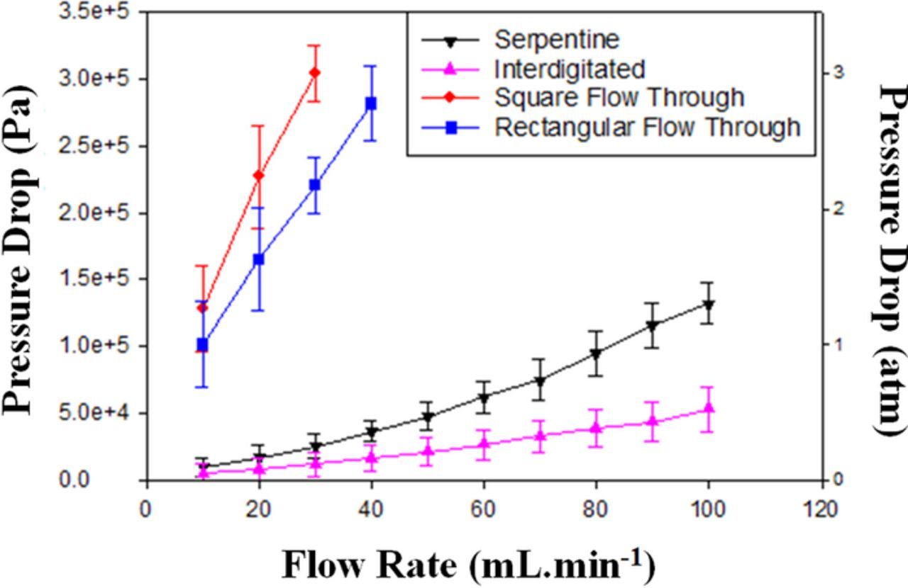
Figure 30. Experimental pressure drop data for serpentine, interdigitated, square flow through, and rectangular flow through flow fields (adopted from Ref. 225).
Many studies have used pressure drop measurements as a key component of their work. Most of these studies are concerned with the flow field design, as this is typically the largest contributor to pressure drop in RFB systems. Xu et al. used pressure drop to calculate power and energy efficiency for a cell with and without engineered flow fields. The study determined that a cell with flow fields has a higher maximum efficiency than one without flow fields.256 Latha et al. compared a serpentine flow field design with an interdigitated design, determining that the interdigitated design was preferable based on lower pressure drop along with better electrochemical performance.257 Houser et al. also conducted a study on serpentine and interdigitated flow fields with a slightly different result, concluding that, while the serpentine design has higher pressure drop, the most preferable design is dependent on operating conditions and electrode materials.106 It should be noted that the disparate findings of such studies frequently arise from flow field design details including channel-land ratio, channel depth, and similar physical features.
Pressure drop has been used for other purposes in the literature as well, demonstrating its versatility. Dennison et al. used pressure drop as a means of evaluating the effect of laser perforated electrodes on a single cell with different flow fields, finding that pressure drop was reduced in all cases, but electrochemical performance was only increased for certain flow field designs.258 Reed et al. employed pressure drop as a means of monitoring the operation of a three-cell stack as well as tracking the energy efficiency with regard to stack temperature and current density. The study concluded that at higher current densities, the increased stack temperature results in decreased pressure drop due to lower electrolyte viscosity. The study additionally compares a flow-through and interdigitated design based on pressure drop, finding that lower pressure drop in the interdigitated design makes it preferable to the flow-through design.259
Pressure drop data is easy to obtain, diagnostically useful, and relatively inexpensive, making such an addition valuable for laboratory- and large-scale system study. There are limitations to the information that can be obtained from these simple measurements, however. While an anomalous pressure drop reading can indicate a change related to fluid flow, it cannot explicitly identify a problem. Instead, only likely locations or causes of a system change can be identified. In order to determine the pressure drop of individual components, pressure readings must be taken at a number of different locations, which involves either more instrumentation or a larger number of tests. Pressure drop can also be sensitive to minor oscillations in system pressure, such as the pulsing of a peristaltic pump, which create unwanted noise and lower the accuracy of the pressure readings. Still, the ease and usefulness of pressure drop data make such a diagnostic relatively high impact with negligible associated complications.
A total energy budget analysis including the pressure drop diagnostics is a common approach to defining the operational energy efficiency of a flow battery. Such analysis can take into account the electrochemical energy efficiency of the system, but also the energy required by ancillary systems such as pumping and heating. The objective of such analysis is to give a more complete picture of where losses in the system exist and to provide context for design considerations and operating conditions which have a system-level impact in addition to cell-level impacts. Electrochemical energy analysis involves simply comparing the energy that goes into a cell during charging and the energy that is discharged from a cell. These values can be used to define electrochemical energy efficiency, described in Eq. 19. A system-level energy analysis expands on the electrochemical charge and discharge energy capacities by incorporating the energy requirements for ancillary systems during both steps. The energy required for ancillary systems during charging is added to the electrochemical energy into the cell, while the energy required by these systems while discharging is subtracted from the energy out of the cell. This provides system level energy efficiency, described in Eq. 20, which can be compared to the electrochemical energy efficiency to better understand the impact of these ancillary systems on cell operation.
![Equation ([19])](https://content.cld.iop.org/journals/1945-7111/165/5/A970/revision1/d0019.gif)
![Equation ([20])](https://content.cld.iop.org/journals/1945-7111/165/5/A970/revision1/d0020.gif)
Energy analysis has been employed at various levels of detail to examine a number of different systems, in terms of design, as well as in terms of chemistry. Khazaeli et al. modeled the energy efficiency of a stack at different flow rates and current densities.260 Reed et al. investigated stack performance by examining the impact of several operating parameters on system energy efficiency. The study examines the impact of current density, flow rate, flow field design, temperature, electrode configuration, and membrane selection on the overall energy efficiency of the system, making it one of the most complete energy analyses done on a full stack.259 The use of woven materials (e.g. carbon cloth) as electrodes for VRFBs has also been explored with energy analysis as well as pressure drop measurements.261–263
Studies have also shown energy analysis as an effective method of assessing electrode performance based on morphology and treatment. Tucker et al. employed such an analysis to assess the optimization of electrodes in a hydrogen bromine flow battery, concluding that increased hydrogen pressure in conjunction with catalyst deposition on the membrane instead of the electrode led to better performance.264 Chen et al. performed another such analysis in VRFBs on electrodes that had been treated by atmospheric pressure plasma jets. The study concluded that such treatments could lead to a 14% improvement in system energy efficiency.265
The versatility of such analysis is demonstrated by its use in a number of less common types of studies, as well. Z. Wei et al. used such an analysis to examine a VRFB with forced cooling of the electrolyte as an ancillary system.266 X. Wei et al. employed this technique to compare microporous separators in a Fe/V flow battery and were able to determine the temperature dependence of the energy efficiency for each of the separators tested.267
While energy analysis is a useful metric for evaluating the losses from individual components within the larger RFB system, it does not provide a high level of data resolution. The individual electrochemical losses cannot be determined with this method and are lumped together into the calculation of electrochemical efficiency. Researchers must be careful to not misattribute a change in performance to the wrong source of losses (e.g. modifying the electrodes, observing improved energy efficiency, and attributing that to kinetics rather than mass transport). Additionally, this approach does not attribute ancillary losses, such as pumping requirements, to individual components, instead using one energy requirement value for the whole system. For these reasons, this type of analysis is most useful when comparing different types of cell components to determine their impact on the electrochemical efficiency, as well as the energy requirements of the ancillary systems and larger system as a whole. It can also serve to highlight areas of importance for improvement in energy efficiency for future research.
Mass spectroscopy
Mass spectrometry (MS) identifies elements and compounds in the gaseous phase based on their molecular weight; it is useful for analyzing and quantifying mixtures of unknown species. MS is conducted by introducing a sample to a mass spectrometer either directly or via a separation device such as a semi-permeable membrane or a chromatography column.268,269 The mass spectrometer then ionizes the sample under vacuum, electrostatically or magnetically separates the various ions by molecular weight, and counts the ions.268 MS is a relevant diagnostic for flow batteries for several reasons, but the most common implementation is for side reaction detection and species identification.
Unwanted side reactions are an inherent performance-restricting characteristic of aqueous-based electrochemical power systems. Operating such systems at elevated voltages can cause unwanted performance loss and permanent degradation via gas evolution reactions or corrosion of the carbon-based electrodes.270,271 These reactions have been numerically simulated and shown to cause negative consequences for the cell including reduced charging current of the charge-storing species, lower efficiency, state of charge imbalance, and capacity loss; in addition, bubble formation within the porous electrodes reduces the active surface area available for reaction and alters transport characteristics within the cell.272–274
MS can be used to identify the onset voltage of such unfavorable conditions and the species evolved. To date, only a few studies have implemented the use of MS as a flow battery diagnostic, with the all-vanadium chemistry being the most commonly studied.275–279 The VRFB, in particular, is susceptible to hydrogen evolution in the negative half-cell and carbon dioxide or oxygen evolution in the positive half-cell. Sun and coworkers investigated gas evolution in an ex-situ experimental setup and found that a porous carbon electrode submerged in fully-charged negative electrolyte can evolve gas without applying any potential, by virtue of the open circuit potential alone (see Fig. 31).275 They calculated hydrogen generation rates and used MS to verify that the evolved gas was predominantly hydrogen. Another study examining hydrogen evolution in negative electrolyte was conducted by Chen and coworkers.276 Their study was more comprehensive as they used an ex-situ experimental setup and MS to quantify hydrogen evolution in V(III) under various negative polarization potentials with different concentrations of sulfuric acid and vanadium.276 Their results suggest that increasing the vanadium concentration decreases hydrogen evolution and the sulfuric acid supporting electrolyte concentration must either be high (3 M) or low (0.5 M) in order to minimize hydrogen generation.276 Another important conclusion from the study came from post-mortem electrode characterization; it was determined that this reaction also results in higher electrical resistance and a change in morphology of the electrode.
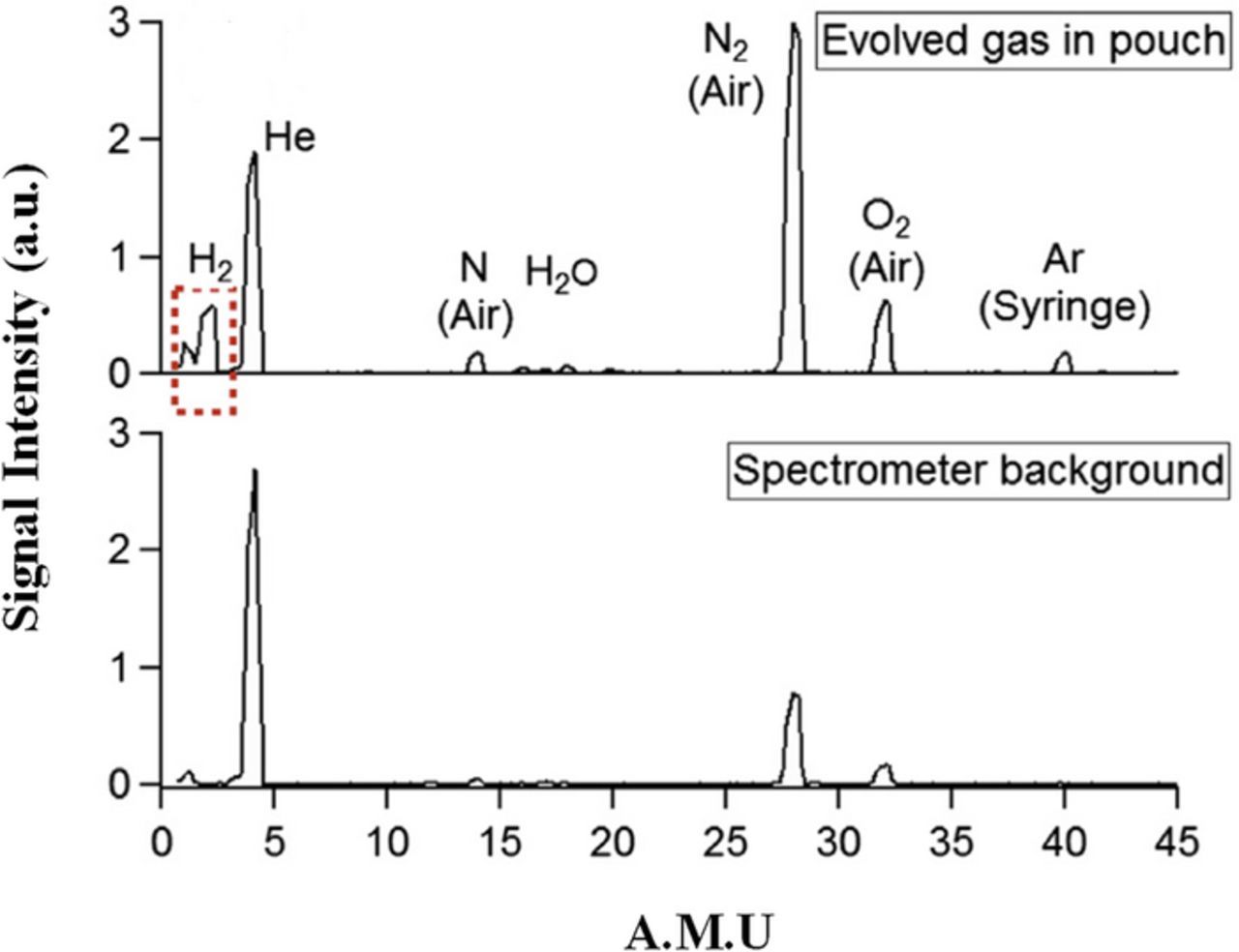
Figure 31. MS has been utilized to identify the evolved gas during VRFB operation (adopted from Ref. 275).
Electrode morphology changes are to be expected on the positive half-cell of VRFBs because the electrochemical potential of V(V) can oxidize carbon at high SoC.270 Liu and coworkers used MS to study this corrosion and oxygen evolution extensively.277 They found that carbon corrosion occurs at lower potentials than oxygen evolution; however, oxygen can be generated at a higher rate than carbon corrosion, depending on electrode material. They also found that the presence of vanadium reduces the corrosion relative to the same sulfuric acid concentration alone. These studies have used MS to investigate electrode degradation, but it can also be coupled with other techniques to provide useful information for researchers. For example, MS has been combined with thermogravimetric analysis to simultaneously analyze electrode mass loss and species deposition on electrodes for a sodium polysulfide/bromine flow battery.278 Another use of combined MS is the work by Nikiforidis and coworkers that used inductively-coupled plasma mass spectrometry to determine cerium content in the electrolyte of a hybrid zinc-cerium flow battery.279 The primary complication in using MS is that it identifies compounds based solely on molecular weight; as such, compounds with identical molecular weights cannot be distinguished. For a VRFB example, molecular nitrogen and carbon monoxide can only be measured as a sum with no differentiation. Thus, fully accounting for all species needs some other technique capable of separating compounds with the same molecular weight such as gas chromatography.
Current distribution
Current distribution is a technique used to obtain two-dimensional, in-plane performance data across the active area of electrochemical cells. By measuring localized current across the active area one can gain useful information regarding the balance between transport and kinetics in-situ. This type of data provides more detailed information than a simple one-dimensional, cell-averaged performance curve. This technique of localized current measurements is not a new concept, in fact it has been studied extensively in fuel cells.280–282 However, recently the diagnostic has been implemented in flow batteries by several groups.106,283–286
There are four primary methods to measure distributed current in electrochemical power systems, three of which have been implemented for flow batteries: hard-wired resistor network, printed circuit board (PCB), and potential probes. The fourth, incorporating Hall effect sensors, has been extensively used in fuel cells and is included here for a complete comparison of measurement techniques. Each approach has its respective advantages and disadvantages, as well as specific hardware requirements and modifications, which are summarized in Table IV.
Table IV. Comparison of measurement techniques for localized current measurements.
| Measurement Technique | Advantages | Disadvantages | Specific Hardware Considerations | Ref. |
|---|---|---|---|---|
| Resistor Network | • Can be passive (shunt resistors), or active (individually controlled segments) |
|
|
285 |
| Printed Circuit Board |
|
• Relatively higher cost |
|
283,284 |
| Potential Probes |
|
|
• Special gasket considerations to accommodate probes | 286 |
| Hall Effect Sensors |
|
|
|
287 |
Hall effect sensors work by measuring the magnetic induction of the magnetic field surrounding an electric current.287 In terms of the cell hardware, the Hall effect sensor approach is the same as a resistor network; both rely on a hard-wired network of connections. In each case the sensors are connected directly (either embedded or via wire) to the back side of the flow field plate. The resistor network measurement technique functions by measuring a voltage drop across a shunt resistor and converting it to a corresponding current. Hsieh and coworkers used this approach to investigate distributions in a VRFB with a flow frame architecture, carbon felt electrodes and two different types of flow plate segmentation hardware.285 However, they found that this approach can result in additional contact resistance and lower spatial resolution because of the need for electrical connectors.285 A potential improvement to this approach is to independently control each connection with a multi-channel potentiostat.280
The PCB approach operates on the same principle as a resistor network via use of shunt resistors; however, the hardware requirements highlight the differences between the two. A PCB eliminates the need for hard-wired connections to the flow field plate by having the resistors and connections built into the PCB, which is placed between the flow field plate and current collector. This aspect allows the PCB to achieve much higher spatial resolution, which can aid in correlating the distribution to transport within the cell. Clement and coworkers have implemented the PCB approach to measure current distributions in a VRFB with a flow channel architecture.106,283,284 These studies have examined several cell and operating parameters including electrode materials, flow rate, compression, and a comparison between serpentine and interdigitated flow field designs as shown in the following figure (Fig. 32).106,284
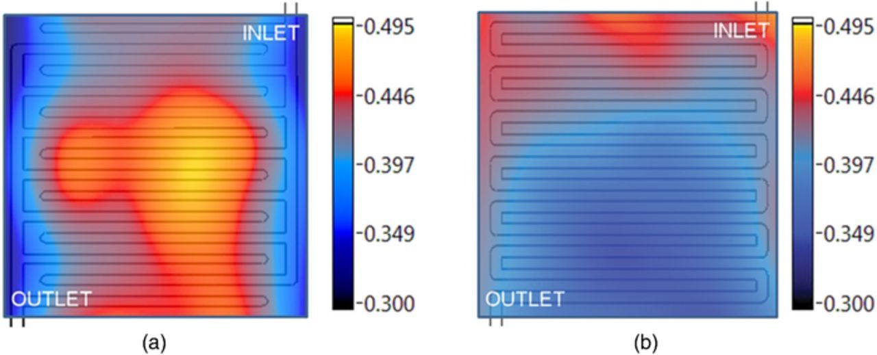
Figure 32. Current distribution measurement for (a) interdigitated flow field, (b) serpentine flow field at 400 mA cm−2. (Ref. 106).
One important hardware consideration for each of these three approaches is the need for fully-segmented flow field plates.280,283–285 With a solid, electrically-conductive flow field plate (typically graphite), current passing through tends to spread laterally within the plate such that a distribution measured at the current collector. This results in a distribution not matching that which is generated in the electrode, and has been shown to be inaccurate even through a plate thickness down to 1.5 mm.283,284 Compression is another important hardware consideration; with a hard-wired network, electrical connections must come from the back of the flow field plate through the compression plate.285 This often necessitates the use of two different materials, which can lead to non-uniform compression. A PCB, on the other hand is uniformly compressed between the flow plate and compression plate.284
The fourth measurement technique of using potential probes is a relatively new approach and doesn't require any flow plate segmentation. In essence, this method uses the electrode and flow field plate as a shunt resistor by measuring the solid-phase potential drop between the electrode and current collector of one half cell.286 Becker and coworkers used this approach to measure current distributions in a flow frame VRFB with carbon felt electrodes under different compressions and flow rates.286 The one caveat with this measurement approach, however, is the assumption that the initial transient current, reported as "dynamic current," is uniform across the active area.286 Becker and coworkers point out that this approach is less expensive than the others and can be implemented in larger cells more easily; however, other issues include lower spatial resolution, probe placement repeatability between builds, and perhaps higher contact resistance.
Multicell stack level diagnostics
Shunt current measurement
In general, individual cells in a stack share a common manifold system at both positive and negative sides. Because of the electrically conductive electrolyte and the potential difference across bipolar plates separating individual cells, shunt currents (shown schematically in Fig. 33) can occur during operation. Shunt currents are considered parasitic losses that cause coulombic loss during the charging/discharging process. These losses can also be present under open circuit conditions because of the transport of electroactive ions (i.e. vanadium ions in VRFBs) by diffusion.288 In order to avoid shunt currents, thinner and longer manifold designs or spirally inlets can be employed. However, this technique is unfavorable as it increases the pumping power required. To avoid elevated pumping loss, understanding of shunt current contributors can lead to manifolds that achieve adequate flow distribution among cells without incurring large additional pumping cost.289–294
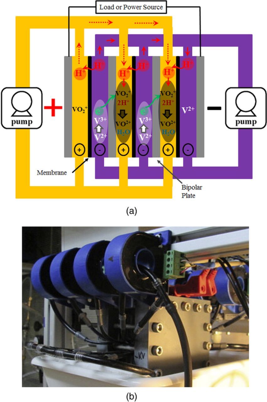
Although shunt currents have been investigated in various systems including bipolar electrolyzers,295 alkaline fuel cells,296 direct methanol fuel cells,297 hybrid sulfur electrolyzers,298 and iron-chromium redox flow batteries299 there are limited publications regarding shunt currents in other RFBs. The majority of publications are mostly focused on model development; however, an experimental procedure has recently been proposed for the measurement of shunt current in a VRFB stack.300 The measurement technique is based on tracking voltages and currents among the individual cells over a range of operation states for a system incorporating an external manifold.
Distributed diagnostics for individual cells within the stack
One of the most important experimental diagnostics is the measurement of voltage and temperature distributions across multi bipolar plates within the RFB stack. For an operating cell, due to the uneven electrolyte distribution across multiple bipolar plates, the solid-phase potential and temperature of individual cells might differ significantly. Therefore, potential probes and sensors to measure the in-plane and through-plane distributions of individual cells are desired. Through application of such probes, the performance of individual cells can be measured via performance characterization and EIS diagnostics. A comparison of EIS technique for individual cells and full stack of PEM fuel cell is reviewed in other References 302,303.
Material characterization
Scanning electron microscope (SEM)
Scanning electron microscopes (SEM) characterize materials on micro and nanoscale resolutions using a focused beam of electrons. The three-dimensional images allow analysis of topographical and morphological features, as well as limited insight into material composition. SEM is commonly used for analysis of electrode surface fractures, chemical composition, identification of crystalline and carbon nanotube structures, nano-engineered surfaces, and investigating membranes.304–309 A typical SEM image has been shown in Fig. 34 demonstrating nanostructured electrode materials for electrochemical capacitor application (Ref. 310).
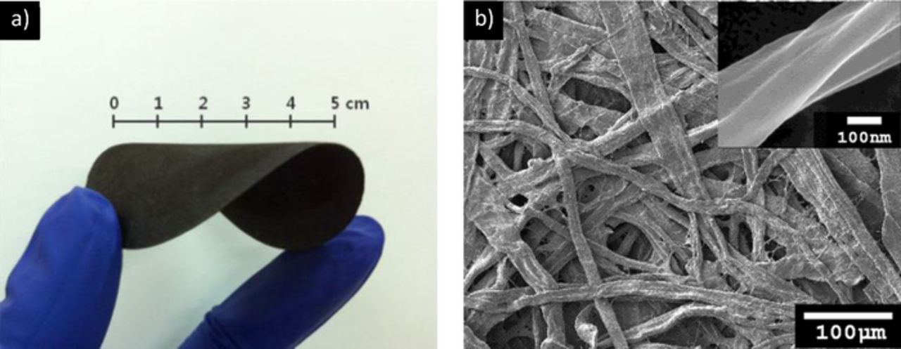
Figure 34. Nanostructured Electrode Materials for Electrochemical Capacitor Applications (Ref. 310).
Although SEM provides high resolution (to 1 nm) images, the diagnostic technique is generally limited to conductive materials; in some cases, sputter coatings can be used to provide the required conductivity for insulative materials like membranes. Additionally, analysis via SEM is complicated by the potential for surface preparation to leave artifacts on electrode materials, the need for specialized training, and high equipment cost. Additionally, much of the information typically gained via SEM is qualitative in nature, though efforts have been made to quantify features in the micrographs.
Energy dispersive X-ray spectroscopy (EDS)
When combined with SEM, transmission electron microscopy (TEM), or scanning transmission electron microscopy (STEM), energy dispersive X-ray spectroscopy (EDS) is used to provide elemental analysis on areas as small as several nanometers in diameter. When materials are subjected to an electron beam, X-rays are ejected which have energy levels specific to the elements present on the material surface. These data are used to map the elemental distribution and to determine the elemental composition in small areas. Figure 35 is a representative EDS spectrum showing peaks correlated to several elements.
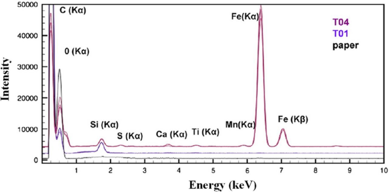
Figure 35. EDS spectra of black toner samples with different elemental profile (Ref. 311).
The y-axis shows the intensity of X-rays (number of X-rays received and processed by the detector; sometimes referred to as Counts) and the x-axis shows the energy level of those counts. These data are then compared with known elemental fingerprints to match to specific elements. EDS is used in membrane, electrode, and electrolyte analysis in VRBs.312–314
In EDS, samples must be flat, homogeneous, and vacuum compatible, thus electrolyte analysis is not done on the actual electrolyte, but often on deposits after the electrolyte is evaporated or otherwise removed. Additionally, size limitations exist and repeated surface analysis may result in beam damage to the sample. Spatial resolution is relatively low when compared with SEM and TEM resolutions (see Table V). Accuracy of measurements range from +/−1% to +/−5% depending on how much a sample deviates from being flat and homogeneous.
Table V. Comparison of different material characterization techniques.
| Sample | Primary | Spatial | Detected | |||
|---|---|---|---|---|---|---|
| requirements | excitation | resolution | depth | Quantitative | Ref. | |
| SEM | Conductive | NA | 1 nm | NA | NA | 365–368 |
| Raman | Conductive or insulating | Laser | 2 μm | 0.2–10 μm | Poor | 369–372 |
| EDS | Conductive or insulating | Electron | 1 μm | 1 μm | Yes | 368,373,374 |
| (a conducting surface coating must be applied) | ||||||
| XPS | Conductive or insulating | X-Ray | 10 μm | 10 nm | Semi | 327,375–377 |
| XTM | Conductive or insulating | X-Ray | 50 nm | Not limited | Yes | 337,339,340,343 |
| FTIR | Conductive or insulating | IR | NA | NA | Yes | 347,348 |
Raman spectroscopy
Raman spectroscopy is a contact-free analytical technique that uses an analysis of scattered light to characterize molecular vibrations. The results are frequently compared to fingerprints and provide detailed structural and molecular data specific to the material analyzed. In this context, Raman spectroscopy is used for carbon electrode and VRFB electrolyte characterization.315–318 Figure 36 includes a schematic of a Raman spectrometer and results showing characteristic peaks in a sample.
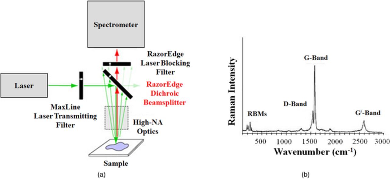
Figure 36. Raman spectroscopy, (a) Schematic of the set-up, (b) An example of a Raman Intensity spectrum (Ref. 319).
The results of Raman spectroscopy yield both an intensity and bands at particular wavenumbers that correlate to specific material properties. Raman spectroscopy yields a weak signal which requires sensitive instrumentation and is subject to laser-derived signal interference. Advantages include the ability to analyze solid and liquid materials through both polymers as well as glass. Additionally, Raman spectroscopy is non-destructive and is performed quickly.
As with other techniques that focus an energetic beam on a sample, increasing the laser strength can damage the sample or introduce artifacts. Additionally, impurities on the surface (e.g. electrolyte components not properly washed off) can fluoresce, interfering with the Raman spectrum. The presence of metal oxides or pure metals can provide an unexpectedly intense response or no response at all, respectively. Such behavior is a concern in RFB systems with metal or metal oxide particles intended to catalyze desirable reactions or inhibit side reactions. A disadvantage of this technique is that only a small area is observed and therefore, multiple measurements are required to satisfactorily characterize the electrode.
X-ray photoelectron spectroscopy (XPS)
X-ray photoelectron spectroscopy (XPS) is a surface-sensitive technique in which a sample is irradiated with X-rays under ultra-high vacuum in order to determine the surface composition. The incident X-ray beam results in the emission of electrons from the sample and a detector records the energy of these emitted electrons. The binding energy is calculated as the energy of the emitted electron subtracted from the energy of the incident X-ray. Typical data output is in the form of a spectrum with intensity plotted against the binding energy. Each element has a characteristic binding energy; for example, oxygen typically exhibits a binding energy of 532 eV and carbon, 285 eV. An example of these peaks is shown in Fig. 37a. With XPS, one can quantitatively determine the elemental ratios of all elements present other than hydrogen, as most XPS instruments do not detect hydrogen in practice. The obtained spectra can also yield information about the chemical nature of the elemental species, as the environment around the element of interest slightly affects the binding energy. This is clearly seen in Fig. 37b, where multiple peaks are observed in the region characteristic of carbon, suggesting many different types of bonded carbon atoms.
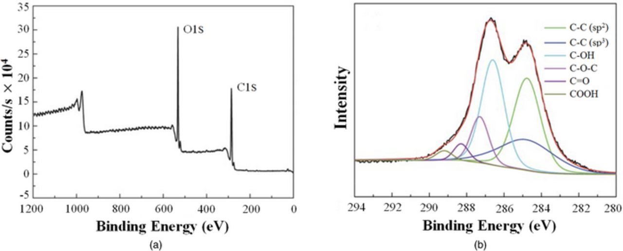
Figure 37. Representative XPS measurement for an electrode composed primarily of carbon and oxygen, with participation of hydrogen in functional groups, (a) general spectra, (b) curve fitting (both figures have been adopted from Ref. 320).
With respect to RFBs, XPS has primarily been applied to the study of electrode surface chemistry. Many studies attempt to correlate kinetic activity with surface chemistry in order to better understand which types of functional groups enhance the kinetic activity of the electrode.147,321–325 Other studies have used XPS to understand how the surface chemistry of the electrode changes when subjected to specific operating conditions, especially in the context of degradation.119,326–328 XPS has also been applied to gain insight into the fouling process in ion exchange membranes used in all-vanadium redox flow batteries and polymer electrolyte membrane fuel cells.224,329,330
Given that the chemistry of the electrode surface, not the bulk carbon fiber, affects redox kinetics, XPS is valuable as a tool to study carbon electrodes because it is a surface-sensitive technique. The emitted electrons from the sample that reach the detector are from the outermost few nanometers of the sample. If the sample is electronically insulating, charging effects may occur that can shift the apparent binding energy of the sample. With the conductive carbon used for electrode materials, this is a minor concern; however, for membrane samples, one must account for such effects. The curve-fitting that is commonly applied to XPS data, shown in Fig. 37b, must also be carried out carefully, with care taken to ensure that each fitted curve is physically meaningful. The full width at half maximum should be consistent for each peak within the fitting for one element. Additionally, if a peak is attributed to a certain functional group, there should be evidence of that functional group in the spectra of each of the constituent elements. For example, if one suspects a COOH group, it should be present in both the C1s and O1s spectra. Due to these considerations, XPS is frequently paired with other techniques that can support elemental composition conclusions. Readers are encouraged to refer to other reviews focused on the XPS technique for further details.331,332
X-ray tomographic microscopy (XTM)
X-ray tomographic microscopy (XTM) is a technique that provides detailed information regarding the 3D microstructure of samples. X-ray tomography has been widely used in biology, radiology and biomedical applications. Recently, the application of XTM for analyzing electrodes used in electrochemical devices has increased significantly. A simplified schematic of the XTM set-up is shown below.
As shown in Fig. 38, the sample of interest is placed on a rotating stage between an X-ray source and a detector. The detector conventionally includes a scintillator that converts transmitted X-rays to visible light while a charge-couple device (CCD) camera captures the resultant 2D image. 2D, cross-sectional images are usually collected several hundred times for high-resolution imaging as a function of various spatial orientations of the sample. The 2D images are reconstructed to form a 3D tomogram showing the micro or nano structure of the sample using numerical algorithms.333,334
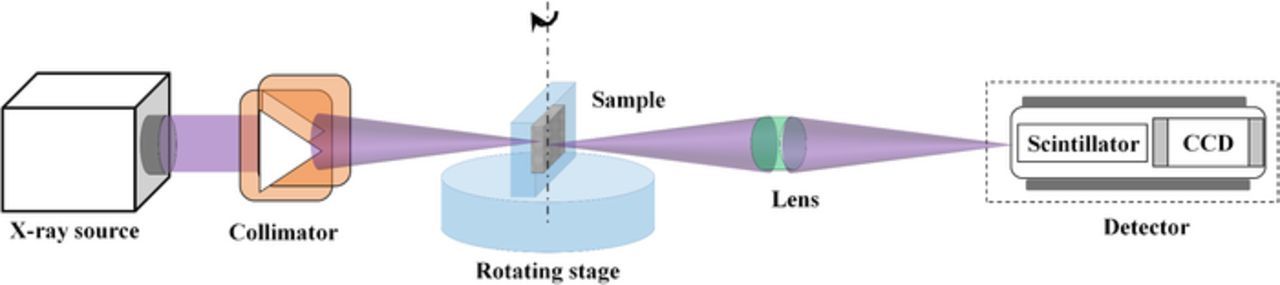
Figure 38. Schematic representation of a XTM set-up.
Since XTM provides detailed information about the interior structure of samples and has relatively high sensitivity to carbon, several studies described ex-situ reconstruction of gas diffusion layers' 3D structures.335–338 Figure 39 includes 3D structure of Toray (TGP-H-060) carbon paper reconstructed based on tomograms at three different compression levels.335

Figure 39. Reconstructed 3D images of Toray (TGP-H-060) carbon paper at three different compression levels of original thickness (a) 73.82%, (b) 69.49, (c) 66.78% (Figure taken from Ref. 335).
High sensitivity to liquid water, no requirement of vacuum (as opposed to SEM and TEM), and high spatial resolution (∼50 nm) are all benefits of XTM. Real-time imaging of two phase flow and liquid water formation in polymer electrolyte fuel cell gas diffusion and catalyst layers has been explored using XTM.339–344
Commonly used electrodes for RFBs have also been reconstructed in 3D using XTM; these results can be incorporated in electrode pore-scale transport modeling.118,345 Being non-destructive, XTM has enabled investigation of electrode degradation for all-vanadium redox flow batteries.327 The majority of XTM applications for RFBs have focused on ex-situ analysis of the electrodes. Recently, a novel miniature cell was demonstrated for quasi-operando XTM imaging of RFBs as shown in Fig. 40.346
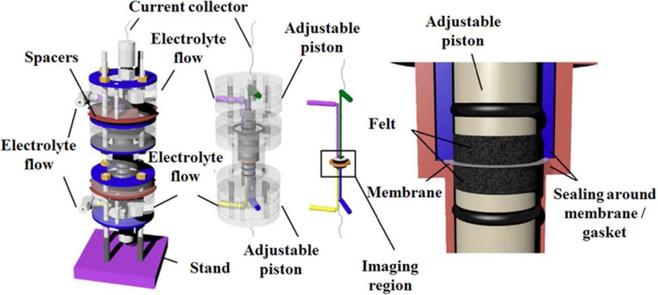
Figure 40. Miniature cell for quasi-operando XTM imaging of electrolyte flow.346
The cell shown in Fig. 40 was fabricated with polypropylene to maximize X-ray transmission. The adjustable pistons of the cell shown in Fig. 40 enable control of electrode compression. Imaging the flow within the cell can be conducted in a lab environment as well as the TOMCAT beamline of the Swiss Light Source synchrotron.346
The major drawback to this technique is the requirement for a sophisticated set-up to collect high resolution images. Additionally, reconstruction of 2D images into a tomogram is computationally expensive. Finally, temporal resolution is limited by material durability to x-ray-induced degradation. As an example, the TOMCAT facility was used to analyze water transport in polymer electrolyte fuel cell gas diffusion layers and is considered limited to an image frequency of 10 Hz to minimize degradation of carbon electrode materials; at 10 Hz, a 3D tomogram would require ∼10 s to collect, averaging all phenomena over that time period.344
Fourier transform infrared spectroscopy (FTIR)
Fourier Transform Infrared Spectroscopy (FTIR) is capable of identifying molecular bonds and structures in a sample of interest. A simplified schematic of a FTIR set-up is shown in Fig. 41. FTIR utilizes infrared (IR) radiation as the primary excitation source; absorption of IR radiation over a wavelength spectrum is used to identify molecular structure. Absorbed IR energy induces elevated vibrational states for the bonds in a molecule; particular IR absorption spectra correspond to particular molecular bonds, enabling molecular identification.347 The FTIR detector (IR sensor) records the intensity of transmitted radiation signals as a function of wavelength in the form of an interferogram. Computer algorithms convert the interferogram to an IR absorbance spectrum using Fourier transformation.
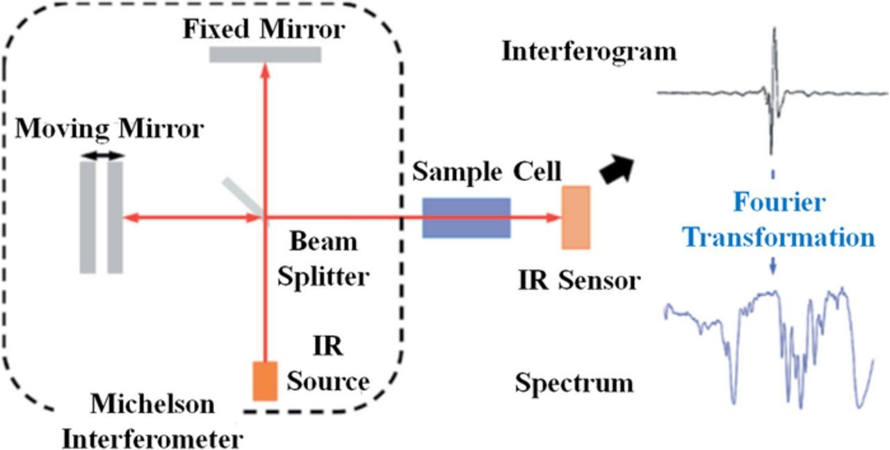
Figure 41. Schematic of FTIR microscopy (Adopted from Ref. 348).
A typical FTIR spectrum, Fig. 42, demonstrates that the intensity of transmitted IR spectra are plotted versus wavenumber (reciprocal of wavelength) with peaks corresponding to various molecular bonds within the structure. FTIR can identify all three material phases (solid, liquid and gas) of a sample. Additionally, quantitative assessment of concentration of particular bonds is possible via calculating the area underneath the characteristic absorption peaks and calibration with a known concentration of the substance of interest.
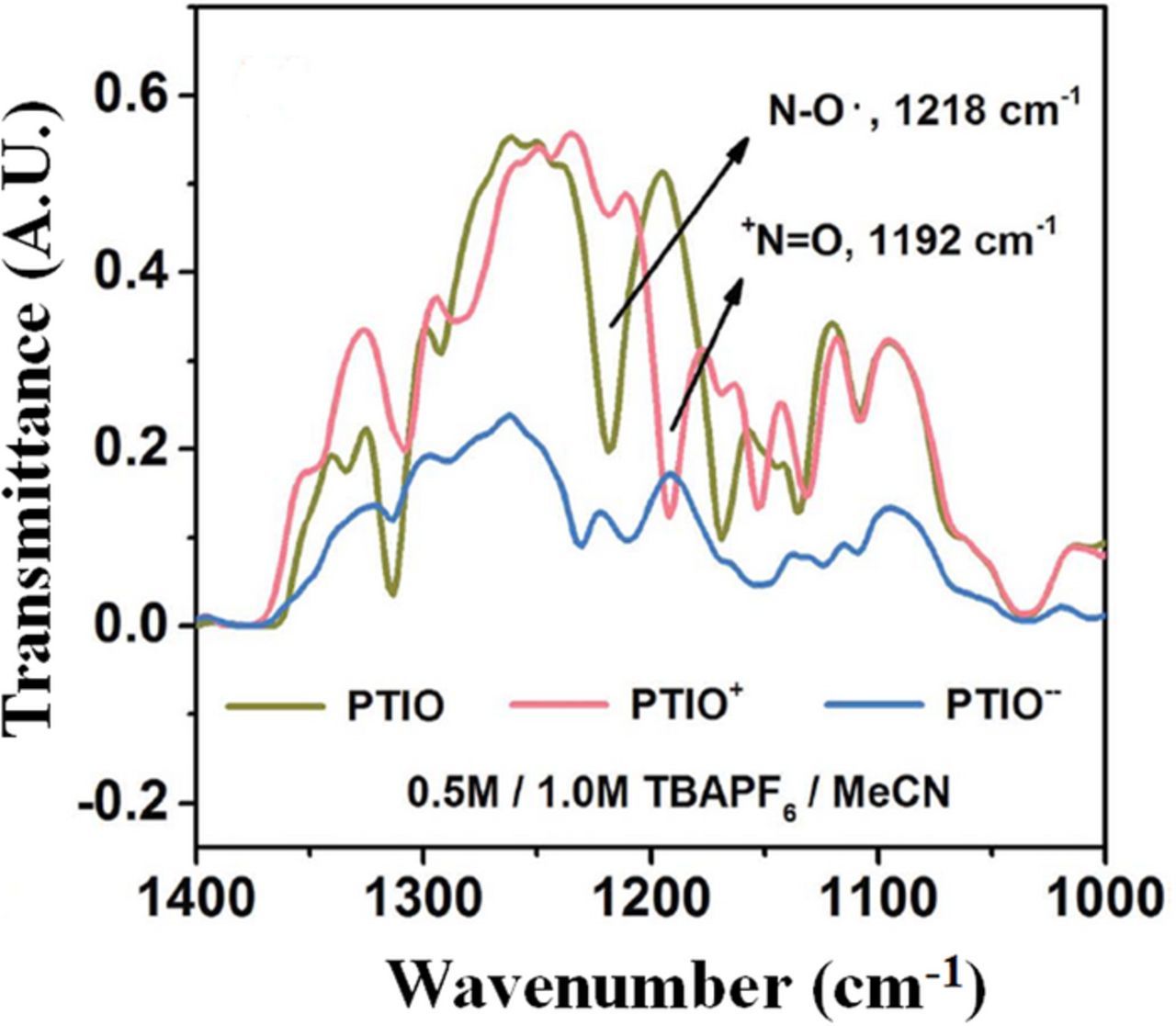
Figure 42. FTIR spectra of 2-phenyl-4,4,5,5-tetramethylimidazoline-1-oxyl-3-oxide (PTIO) species within organic solvent (adopted from Ref. 156).
Extensive utilization of FTIR spectra is reported in the literature for electrochemical energy devices, e.g. analyzing novel membranes for RFBs with FTIR.349–354 FTIR has also been used for investigating the surface properties of as-received and modified/treated carbon electrodes.355–358 FTIR is predominantly used ex-situ, in which the sample of interest is placed inside the instrument. However, in-situ utilization of FTIR has also been demonstrated as a real-time sensor for measuring the state of charge in an operating RFB system.156
Although FTIR samples can be electronically conductive or non-conductive, sample preparation requires salt plates in the set-up; thus, samples must be compatible with such materials. Carbon dioxide and water vapor present in the lab environment can also create false signals; therefore, initial purging with nitrogen is required before the start of analysis. In general, FTIR does not provide local composition information, but rather measures a composite response characteristic of an entire sample. Also, some low frequency molecular vibrations require powerful spectrometers capable of scanning in far IR-regions (20–400 cm−1) to attain acceptable signal to noise ratio.347,348
Brunauer-Emmett-Teller (BET) surface area assessment
The Brunauer-Emmett-Teller (BET) method is used to measure the surface area of a material by physical adsorption of inert gas molecules such as nitrogen or carbon dioxide. The BET method utilizes a multilayer adsorption model based on the adsorbate gas following the Langmuir adsorption model at each layer of adsorbed gas molecules. To measure the BET surface area, one loads sample into a sealed vessel, which is then evacuated. The sample is exposed to several pressures, and the pressure versus volume of adsorbate gas can be fitted to the BET equation to obtain the effective surface area of the material. Information about the pore size distribution may also be obtained.
Although the BET method has been used to measure the surface area of carbon electrodes in RFBs,321,359–361 and capacitive water deionization,362 one must note that nitrogen physisorption may not accurately capture the surface area and pore size distribution. The area measured with nitrogen adsorption BET often conflicts with the area found using another gas or determined via another method. The use of carbon dioxide as the adsorbate has been suggested as a plausible alternative for VRFB applications due to carbon dioxide reaching the pores accessible to vanadium more similarly than nitrogen.363 Other work has used X-ray micro-tomography to find the electrode surface area,327 although this method is not widely available. In-situ electrochemical measurements including impedance spectroscopy and cyclic voltammetry in a sulfuric acid solution can be carried out to find the capacitance of the electrochemical cell, and if the specific capacitance of the electrode is known, one can then find the effective surface area.149,275 One should note that the specific capacitance of the carbon can be affected by the presence of functional groups, complicating efforts to use results found in the literature.364
A comparison of different material characterization techniques is summarized in the following.
Discussion
In Table VI, the previously-introduced diagnostic techniques have been summarized, highlighting the most frequent technique for each loss category. In the following table, the corresponding techniques have been color coded (colors available online) based on the frequency of their applications within the list of papers considered. Generally, a combination of multiple techniques is used to diagnose cell behavior after some modification to materials or conditions, often in through the lens of inefficiencies.
Table VI. Techniques and associated losses in the cell (Darker backgrounds indicate higher frequency reported in the works cited in this review).
Table VI can serve as a starting point for choosing diagnostic techniques that an investigator may employ to study losses in RFBs. When designing an electrochemical system, there are tunable parameters for every component of the system that can be engineered to optimize the performance metrics. Table VII serves as a companion to Table VI by summarizing RFB components and the properties of these components that can be manipulated to influence the losses summarized in Table VI. Thus, investigators interested in improving kinetic losses in a flow battery can utilize a variety of diagnostic techniques (suggested in Table VI) to assess responses to changes in electrode properties (summarized in Table VII). Depending on the modifications or improvements investigated, some investigative techniques may have limited utility or insight.
Table VII. Variables and tunable parameters within the different components of an electrochemical systems.
| Component of the RFB system | Variables and tunable parameters | ||
|---|---|---|---|
| Electrolyte | Concentration of redox active material | ||
| Supporting Electrolyte | |||
| Solvent Type | |||
| State of Charge (SoC) | |||
| Electrochemical Operating Conditions | Constant voltage | ||
| Constant current | |||
| Potential sweep | |||
| Electrochemical Reactor | Membrane | Type | Polymeric (type and equivalent weight) |
| Non-polymeric and Porous | |||
| No-membrane (co-laminar configuration) | |||
| Conductivity | |||
| Permeability | |||
| Selectivity | |||
| Degree of reinforcement | |||
| Flow plate | Flow plate Geometry | Serpentine | |
| Interdigitated | |||
| Flow-through | |||
| Parallel | |||
| Parallel-serpentine | |||
| Mesh | |||
| Spiral | |||
| Foam | |||
| Hybrid and nature-inspired | |||
| Channel Geometry | Depth | ||
| Width | |||
| Length | |||
| Shape | |||
| Material | Conductivity | ||
| Porosity | |||
| Corrosion resistance | |||
| Electrode | Material | Carbon felt | |
| Carbon paper | |||
| Non-carbon | |||
| Porosity | |||
| Permeability | |||
| Tortuosity | |||
| Wettability | |||
| Surface Area | |||
| Catalytic activity | |||
| Conductivity | Electrical | ||
| Thermal | |||
| Multiple cells (stack) | Manifold | Design | |
| Position (internal/external) | |||
| Cell configurations | |||
| Physical Operating Conditions | Flow rate | ||
| Temperature | |||
| Flow configuration | Co-flow | ||
| Counter-flow | |||
It is likely in any system that contributions to inefficiency, performance loss, and degradation come from multiple components and conditions; indeed, the goal of these diagnostic techniques is to delineate and quantify those contributions. As a result, it is important to understand how the stages of the design process can be correlated to inefficiencies and map them to the various sources of losses. A diagram has been formulated and is shown in Fig. 43, correlating the system components and design parameters to their respective loss mechanisms and which performance metrics are relevant for each.
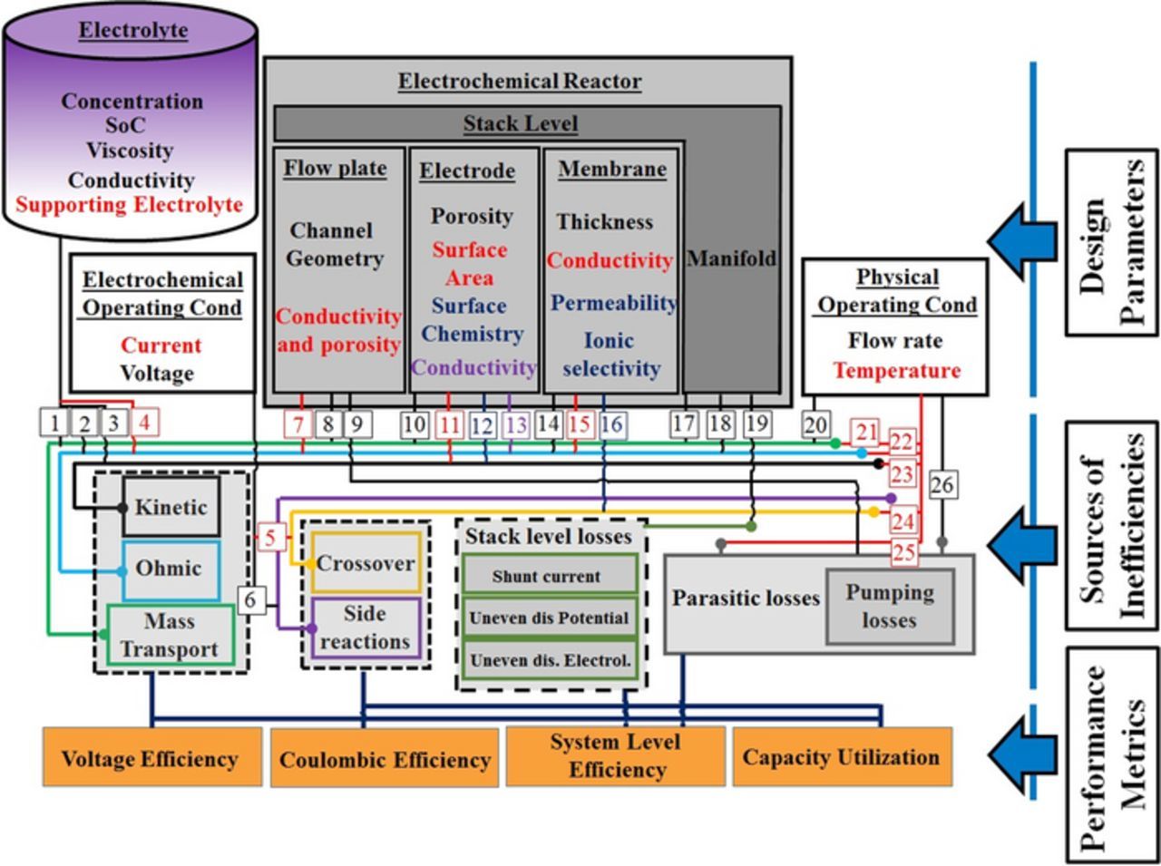
Figure 43. Schematic representation of the connection of components and different losses (color image is available online and the variable tags/numbers are explained in the text).
Figure 43 is broadly organized into three sections: the upper section includes aspects of the RFB that can be chosen or designed, including physical components and operating conditions; the middle section has groups of losses or contributions to inefficiency, at cell and system levels; the bottom section then relates these to the overall metrics employed to study those losses as functions of the design considerations chosen. The color coding in Fig. 43 aids in relating these three categories. To use Fig. 43, one can identify tunable design parameters, e.g. membrane thickness (assigned #14) and conductivity (#15); both are mapped to ohmic losses (blue color) which affects voltage efficiency. Note that conductivity and thickness do not strictly influence coulombic efficiency. However, separator permeability (#16) is mapped to crossover (orange color) in the cell, resulting in it being a parameter that ultimately affects the coulombic efficiency of the system. Figure 43 is thus useful to map the effects of tunable design parameters to corresponding sources of inefficiencies and performance metrics of the cell. A major feature of Fig. 43 is that it provides a bridge between diagnostic techniques and ultimate performance metrics. For instance, if the goal of a study is to increase the coulombic efficiency of a system, diagnostic techniques to assess crossover (orange color), side reactions (indigo color), and parasitic losses (light gray) must be selected; the relevant tunable parameters, then, are separator permeability, temperature, flow rate, voltage, and current.
Establishing the connection between the different components of the electrochemical system to the diagnostic techniques, it is also interesting to summarize the common type of analysis is usually conducted on the electrochemical systems.
Performance characterization of the electrochemical cell
In this section, a short introduction is provided regarding each loss mechanism shown schematically in Fig. 43, focusing on the parameters that can be measured via the above diagnostics. Ultimately, the goal is to elucidate the connections between experimentally-measured parameters and the parameters used for modeling the losses in operating RFBs. In general, as described in Polarization curves section, the Nernst equation is used to model the open-circuit potential of the cell; when faradaic current passes through the cell, the voltage changes due to various sources of overpotential including kinetic, ohmic and mass transport overpotentials.
Kinetic losses (overpotentials)
Kinetic losses due to activation polarization result in a sharp initial overpotential upon the onset of current. Following the initial sharp voltage change, kinetic overpotential increases roughly linearly as current increases, as shown in Fig. 7. Thus, in RFBs operating at low current, reaction kinetics losses often dominate cell overpotential. Usually, utilizing a stable reference electrode enables distinguishing the kinetic overpotentials of negative and positive sides in real-time for an operating RFB.115,124 Depending on the type of the RFB, the negative or positive sides might undergo an ion-intercalation into a host solid; other kinetic models are used depending on the nature of charge transfer mechanism in the negative or positive sides.
Model of electrode kinetics for RFBs under dilute electrolyte conditions
The Butler-Volmer model for heterogeneous reactions is used frequently for correlating the current density of the battery as a function of overpotentials for kinetically controlled RFBs as shown in Eq. 21.143 (Please see Eq. 1 for electroactive species)
![Equation ([21])](https://content.cld.iop.org/journals/1945-7111/165/5/A970/revision1/d0021.gif)
These losses are independent for the negative and positive halves, though the Eq. 21 has been shown only for the negative side of the battery and a similar equation needs to be considered for the positive side (Please refer to Eq. 1). In Eq. 21, negligible mass transport limitation is assumed; therefore, there is no concentration gradient between the bulk solution and the electrode surface ( , x is measured from the surface of the electrode). The general form of the Butler-Volmer equation in Eq. 21 needs to be modified if the surface concentrations of the oxidizing and reducing species differ from the bulk concentrations and readers are encouraged to check the details of such a modification in other references.115,143
In Eq. 21 A is the surface area of the electrode (unit: m2), k0 is the standard rate constant (unit: m.s−1), and α is the dimensionless transfer coefficient (varies from zero to unity). It is common to rewrite a simplified form of Eq. 21 utilizing exchange current in the form of Eq. 22 when overpotential is relatively small.
The exchange current densities ( of many RFB chemistries are in the range of pA/cm2 to 10 A/cm2.
![Equation ([22])](https://content.cld.iop.org/journals/1945-7111/165/5/A970/revision1/d0022.gif)
where Rct is the charge transfer resistance (in ohms) and is the negative reciprocal of the slope on a plot of current density against cell overpotential. Additionally, such a plot yields the exchange current density when the conditions of fast kinetics and minimal mass transport overpotential are met. Often, EIS is used to obtain this same charge transfer resistance.
For large values of overpotential (negative or positive), the Butler-Volmer equation can be cast into the Tafel form, shown in Eq. 23 which can be measured experimentally with relative ease.
![Equation ([23])](https://content.cld.iop.org/journals/1945-7111/165/5/A970/revision1/d0023.gif)
As a result, it is possible to extract the transfer coefficient from the slope of a logi − ηkinetic curve, as well as the exchange current from the y-intercept. This is true if the logi − ηkinetic exhibits linear behavior over some range of current density. Extrapolating the anodic and cathodic linear branches of the Tafel plot (which correspond to charging and discharging reactions for a half cell) results in an intercept of logi0.
It is important to note that if the system is being affected by appreciable mass transport overpotential, a Tafel plot will deviate from linearity at very large overpotentials, sometimes having short or non-existent linear regions. As a result, for the systems in which the normal Tafel plots are complicated by mass-transfer effects, a modified version of the Tafel approximation can be used.143
Experimental approaches can be assembled that give insight into all of the properties that affect kinetic behavior. The surface area of the electrode can be determined ex-situ (most commonly using the BET method) and/or in-situ (via EIS or CV). These methods often result in disparate values for surface area, as described previously. Three approaches are common to assess the standard rate constant (or exchange currents) and/or the transfer coefficient: CV or RDE, in-situ symmetric cells, or EIS.
In the second approach, kinetic parameters are measured in-situ while current is being drawn from the cell.124 Since the current drawn from the cell is small, it is assumed that the overpotential associated with the ohmic and mass-transport to/from the surface of the electrode is negligible. However, the overpotential associated with crossover is also frequently neglected, though this is not accurate in an operating cell. In order to eliminate overpotential associated with crossover at low current density, symmetric cells can be used in which both sides of the electrochemical cell have the same redox species.139,156,378 It is also important to note that, in order to distinguish the activation polarization of the negative versus positive sides in an operating cell, a stable reference electrode must be present.115,124
In the third approach, EIS is applied in-situ and Nyquist plots are obtained at multiple operating conditions. At open circuit, the charge transfer resistance for a practical electrode material and the chemistry of interest can be measured. Measurement of the charge-transfer overpotential enables one to calculate the practical exchange current and, if the electrochemical surface area is known, the kinetic rate constant can be obtained.176 Several studies have used EIS to examine the effects of electrode surface modification on the effective kinetics in RFBs.149,176,379 However, if there exists non-linearity associated with the kinetic overpotential, there is a need to map functional groups of the electrodes along with local performance in order to understand such non-linearity.
Model of electrode kinetics for RFBs under concentrated electrolyte conditions
The phenomenological Butler-Volmer model of electrode kinetics, as described through Eq. 21, has been widely used for several types of RFBs and fits the current-voltage data for these types of batteries very well. However, if the Butler-Volmer model is used for RFBs undergoing non-ideal condition (i.e. ion-intercalation, concentrated solutions, and some others), as described by Eq. 21, there is no term accounting for any non-idealities arising due to the ionic activity coefficient deviating from unity in these systems. This deviation from ideal behavior may also be relevant for highly concentrated systems. Some of the non-idealities that may emerge are configurational entropy, elastic stress, and phase transformations. Therefore, a refined model is required for describing the charge transfer (taking into account these non-idealities) and such an approach will provide a modeling framework for faradaic reactions in ionic solids and concentrated solutions.
An example of such an approach is a model developed by M. Bazant based on non-equilibrium thermodynamics.380 Via this modeling framework, the reaction rate has been modeled as a function of concentration gradient, elastic strain, and surface tension. Bazant's model has been developed by incorporating concentrated solution theory for batteries, fuel cells, and induced-charge electrokinetics; therefore, is applicable for RFBs utilizing concentrated electrolytes of various solutes.381–384 The exchange current is formulated in Eq. 22, modified for concentrated solution.380
![Equation ([24])](https://content.cld.iop.org/journals/1945-7111/165/5/A970/revision1/d0024.gif)
In Eq. 24, γ symbolizes the activity coefficients of reduced and oxidized species (refer to Eq. 1), electrons and transition state species.380 In Eq. 24, Ce is the concentration of free electrons (density of states) and γe is the activity coefficient of electrons. Usually, it is safe to assume that the activity coefficient of electrons is unity; however, under certain conditions, it diverges from unity. The applied elastic/plastic or thermal stress, as well as phase transformation, are major reasons for such divergence.
It is apparent that the first factor is the classical formula developed for exchange current (Eq. 22) and the second factor imposes a modification to the exchange current for concentrated solutions. In the limit of dilute solutions (all activity coefficient equals 1) the exchange current obtained utilizing Eq. 24 yields Eq. 22. Therefore, for concentrated solutions, the exchange current must be modified and the activity coefficients measured via experimental diagnostics. Common techniques for measuring activity coefficients for concentrated solutions utilize electrochemical cells with ion-selective membranes and gas chromatography.385,386
Ohmic losses
Ohmic overpotential in an operating cell is due to both the ionic and electronic resistances, as well as contact resistance between all components. Electronic resistances (from electrodes, flow fields and current collectors) and contact resistances (mostly between electrodes and flow fields) are generally much smaller than ionic resistance (from electrolytes and membrane) when graphitic materials are used as electrodes. To assess the electronic resistivity of different cell components, Ohm's law is used as described in the following equation.115
![Equation ([25])](https://content.cld.iop.org/journals/1945-7111/165/5/A970/revision1/d0025.gif)
Where, jelectronic symbolizes the electronic current density and σeffs is the effective electronic conductivity. The effective electronic conductivity accounts for the porosity of the cell components; this conductivity must be measured at a compressed state (similar to the compression being imposed during cell assembly).115
Ionic current in an electrolytic solution is due to the motion of charged particles as described in Eq. 26.387
![Equation ([26])](https://content.cld.iop.org/journals/1945-7111/165/5/A970/revision1/d0026.gif)
where jionic is the ionic current density (A.m−2), zi is the charge carried by an ion, and NElectrolytei is the flux density of each species (mol.m−2) in the electrolyte. In Eq. 26, all charged species contribute to the ionic current. However, the contribution of various species depends on the magnitude of the flux density for a particular species. The conductivity of the electrolytes and the membrane can be measured using experimental diagnostics.
The most common technique for measuring the conductivity of the electrolytes is via ex-situ conductivity cell as described in Ionic and electronic conductivity measurement section in which the electrolyte conductance is measured via imposing an electric field as described in Eq. 27. Also, in-situ EIS as described in Electrochemical impedance spectroscopy (EIS) section is frequently employed.387
![Equation ([27])](https://content.cld.iop.org/journals/1945-7111/165/5/A970/revision1/d0027.gif)
Modeling the ionic current through the membrane, as described in Eq. 26, requires quantifying flux density for all the contributing ions. The most common approach assumes an infinitely dilute solution. In this theory, the flux of each individual species is modeled assuming only interaction with the surrounding solvent.387
![Equation ([28])](https://content.cld.iop.org/journals/1945-7111/165/5/A970/revision1/d0028.gif)
According to Eq. 28, the flux density of the charged species has contributions from diffusion (first term), migration (second term), and convection (third term). Utilizing membrane characterization techniques, the uptake values of species from the bulk solution to the membrane phase can be obtained; membrane thickness expansion due to exposure to the electrolyte can be measured ex-situ as demonstrated in Ref. 102. Therefore, quantitative assessment of the concentration gradient within the membrane phase (∇cmi) can be approximated with reasonable accuracy. The diffusivity of the various ionic species across the membrane (Dmi) can be assessed as described in section 2.7; among various techniques, the most common approach is utilizing UV/Vis spectroscopy.102,114 Most RFBs utilize concentrated electrolytes to maximize energy density; it is important to note that the diffusivity of individual ionic species for liquid phase RFBs is a strong function of electrolyte composition (e.g. state of charge, concentration of supporting electrolytes, concentration of the solvent); as a result, individual ionic diffusivities may vary greatly from dilute solution conditions. An example of such an approach has been demonstrated in Ref. 114 in which interaction coefficients have been deduced for the diffusivities of individual vanadium ions in a VRFB cell to account for the state of charge dependence of ionic diffusivities. The mobility of individual ionic species within the membrane phase (umi) is usually determined based on concentrated solution theory via experimental diagnostics or modeling approaches as described in Refs. 388,389. An alternative for determining the ionic mobility to be used in Eq. 28 is utilizing Nernst-Einstein relations to correlate the mobility to diffusivity.115,116
To determine the electrostatic potential gradient across the membrane (∇Φm), potential distribution diagnostics, as described in Potential distribution section, can be used. However, due to the complexity of this method, an alternative approach is to correlate the electrostatic potential gradient to the current density drawn from the cell using Eq. 27.113,114 For this approach, membrane conductivity is used via applying in-plane or through-plane conductivity measurement as described in Ionic and electronic conductivity measurement section and formulated in Ref. 387.
The convective term in Eq. 28 requires quantification of solvent velocity (v0) through the membrane. In practice, for aqueous solvents, usually the gradient in chemical potential is neglected and the velocity of the solvent is correlated to the cell current density, electro-osmotic drag coefficient (ξ), and concentration of the solvent within the membrane phase (cm0) as formulated in Eq. 29. Further details are available elsewhere.146,255
![Equation ([29])](https://content.cld.iop.org/journals/1945-7111/165/5/A970/revision1/d0029.gif)
In practice, the solutes within the solvent interact with other solutes as well as the solvent, resulting in error when comparing the description in Eq. 28 to a concentrated solution. In these cases, more sophisticated mathematical models using concentrated solution theory are required to model the species fluxes.388,390
For an operating cell, the overpotential associated with the ionic current through the ion-exchange membrane and the electrolyte usually dominates ohmic loss. EIS can be used to measure the resistance associated with the ion-exchange membrane and the electrolyte solution at any current (as described in Electrochemical impedance spectroscopy (EIS) section); for the membrane, this measurement can be done in-situ or ex-situ, though capturing the electrolyte resistance is far more accurate in-situ. Measuring the ohmic resistance for an operating cell is usually followed by calculating the area specific resistance (ASR) for the cell according to the following equation. ASR is usually reported in ohm.m2 or ohm.cm2.
![Equation ([30])](https://content.cld.iop.org/journals/1945-7111/165/5/A970/revision1/d0030.gif)
Equation 31 can be used to calculate the ohmic overpotential.
![Equation ([31])](https://content.cld.iop.org/journals/1945-7111/165/5/A970/revision1/d0031.gif)
Mass transport losses
Mass transport overpotential is commonly the performance-limiting factor at high current density; referring to Fig. 7, this occurs as the polarization curve deviates from ohmically-dominated linear behavior at high current. Assuming other losses do not lead to cell voltage dropping below a safe cutoff (often in the range of 0.2 V–0.6 V), mass transport-limited current may be reached. However, as noted previously, all sources of overpotential are present at all current densities. Indeed, mass transport overpotential has been found to be significant even at moderate currents well below the onset of mass transport limitation.115,137
The greatest mass transfer rate (and, consequently, overpotential) associated with Aα + occurs when the surface concentration approaches zero, or  so that
  . Theoretically, the limiting current under these operating conditions can be defined according to Eq. 32.143
![Equation ([32])](https://content.cld.iop.org/journals/1945-7111/165/5/A970/revision1/d0032.gif)
In Eq. 32,  is the intrinsic diffusion coefficient of Aα + in solution and δ0 is the Nernst diffusion layer thickness.143 The magnitude of the Nernst diffusion layer thickness is generally unknown; thus, it is convenient to combine the diffusion coefficient with the diffusion layer thickness to define a mass transfer coefficient (
 ) for species Aα +.115 An added benefit of assessing the mass transfer coefficient is that it can readily be found experimentally. Assessing the limiting current enables the calculation of the mass transport overpotential according to Eq. 33.120 However, when using Eq. 33, one needs to consider the major limitation of this approach. Equation 33 includes a 0-D assumption for limiting current for the entire cell. Nonetheless, for an operating cell, the limiting current might be distributed along the entire electrode depending on the species transport mechanism across the entire electrode.
![Equation ([33])](d0033.gif)
Evident in Fig. 43 is that multiple parameters affect mass transport overpotential; primary contributors are flow plate design, electrode morphology, concentration of electroactive species, and flow rate. With so many contributions, multiple measurements should be assembled to assess mass transport losses under a variety of relevant operating conditions. The overpotential can be quantified with EIS by analyzing a Nyquist plot in the low frequency region (often in the mHz range or lower); this resistance can be integrated as a function of current to obtain the mass transport overpotential. While it is relatively inefficient to operate an RFB near mass transport-limited current density, this metric provides a ceiling for system current density. Frequently, the limiting current can be different for the negative and positive sides, thus a whole-cell limiting current is typically found. Mass transport-limited current density can also be different for charging and discharging conditions, as well. The definition of limiting current in this manner includes all the parameters contributing to mass transfer; diffusion from the bulk solution to the electrode surface and convection due to electrolyte flow rate are the most dominant parameters. The limiting current obtained ex-situ using RDE is thus only one component, considering the fact that this technique only quantifies the diffusive effects from the bulk solution to the electrode surface.
Two other relevant mass-transport properties are the effective diffusivity of electroactive species through the porous electrodes and the mass transfer coefficient, as discussed earlier. The intrinsic ionic diffusivity in the electrolyte (e.g.  ) is readily obtained using RDE. However, the intrinsic diffusivity in the electrolyte must be modified in order to account for electrode porosity and pore morphology.391 The most commonly used description of effective diffusivity (
 ) is the Bruggeman relation, shown in Eq. 34.
![Equation ([34])](d0034.gif)
In Eq. 34, ε represents the porosity of the electrode. The application of Bruggeman relation according to Eq. 34 includes the porosity effect but does not include consideration of pore morphology in the effective diffusivity. As a result, a more complex description can be employed that is more accurate, but also requires more information.392,393 An example of such consideration is shown in Eq. 35.392
![Equation ([35])](d0035.gif)
In Eq. 35, Pe is the Peclet number while a and b are empirical parameters determined via fitting experimental data as shown in Fig. 44. Using Eq. 35, effective diffusivity values were deduced experimentally for porous electrodes; the flux of species was evaluated at limiting current for a given concentration of species.392
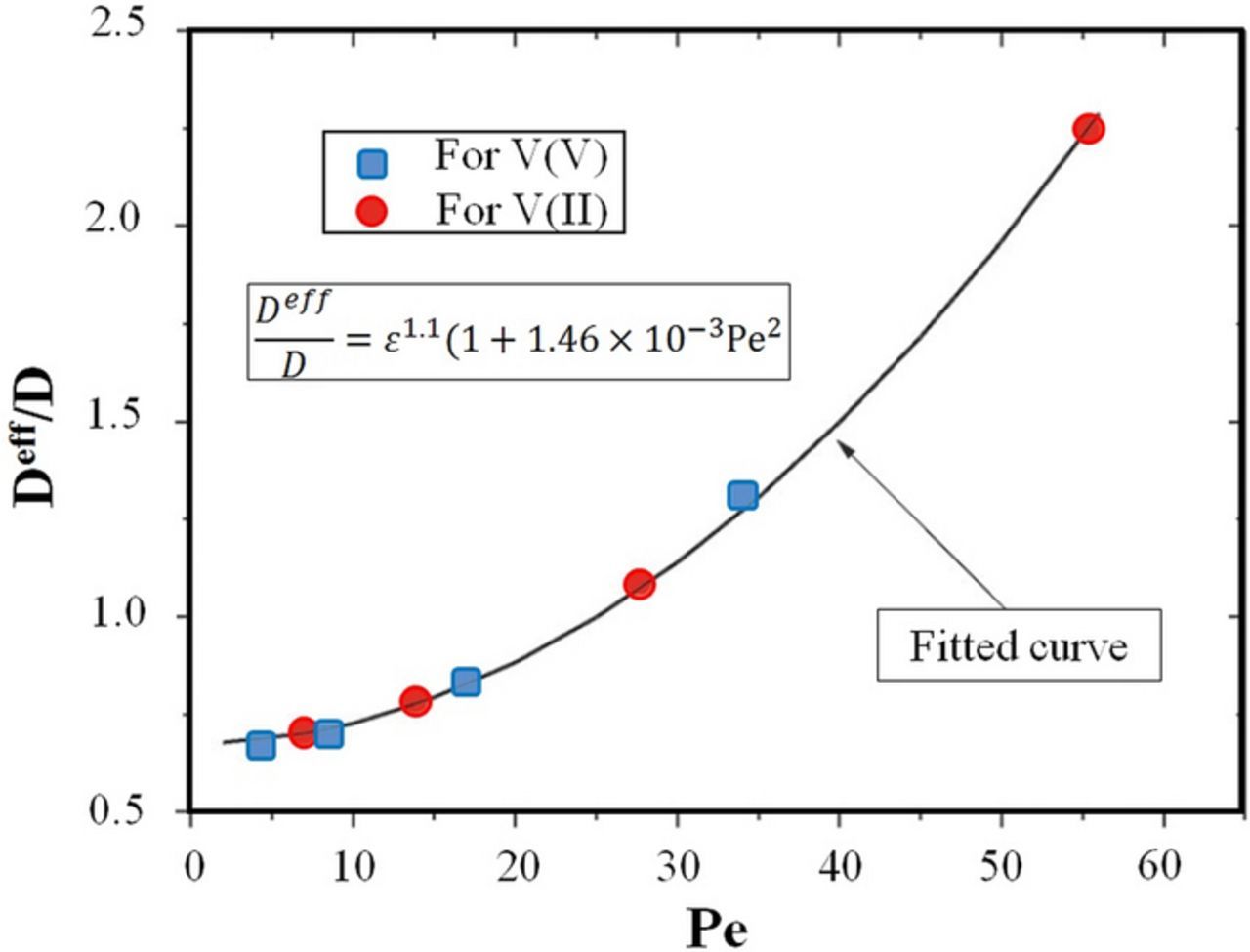
Figure 44. Determining effective diffusivity from fitting experimental data (Figure adopted from Ref. 392).
A similar approach can be employed to determine the mass transfer coefficients based on experimental data. The mass transport coefficient can be approximated using Eq. 36.
![Equation ([36])](d0036.gif)
where x and y are the parameters to be determined via fitting experimental data with vc as flow velocity. Such a treatment has originally been demonstrated in Ref. 394 and more recently in Ref. 395 (Fig. 45a). Similar approach has also been implemented for calculating mass transfer coefficient for different flow field designs under certain operating conditions (Fig. 45b).393
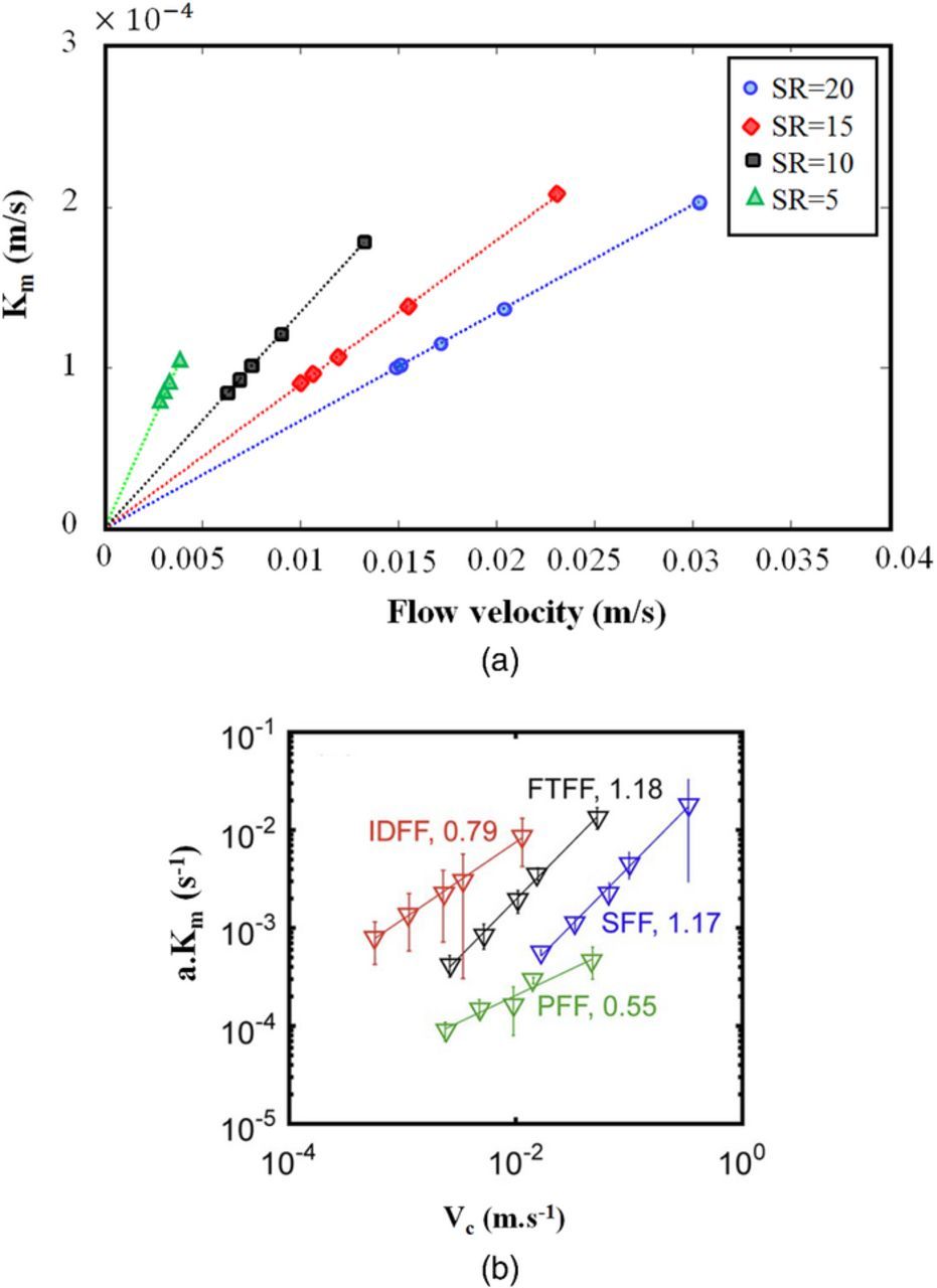
Figure 45. Determining mass transfer coefficient, (a) as a function of electroactive species stoichiometry (the four sets of data refer to different stoichiometric ratios (SR)), Ref. 395 (b) For different flow field designs including serpentine (SFF), interdigitated (IDFF), parallel (PFF) and flow through (FTFF), Ref. 393, Note: Within Fig. 45b "a" is electrode area per unit volume).
Crossover and side-reaction losses
Crossover and side-reaction losses both contribute to decreased coulombic efficiency. As shown in Fig. 43, there are multiple parameters affecting crossover and side-reactions. The most common technique to investigate side reaction onset and behavior is CV; if conducted appropriately, CV directly provides the voltage window range for the particular chemistry that prevents appreciable parasitic reactions, gaseous evolution as an example.42,149,396–398 In practical applications, avoiding overcharge conditions allows near-total mitigation of parasitic side reactions. It is also noted that there have been findings of gas evolution and electrode oxidation at high SoC in some batteries;275 this can readily be avoided by draining the reactors when not actively passing current. However, if the cell undergoes unexpected overcharge conditions, the onset potential for those reactions should be known.
Although parasitic side-reactions are mostly avoidable via operation at appropriate electrochemical operating conditions (predominantly within a prescribed voltage window), coulombic efficiency loss due to electroactive species crossover is inevitable. As was shown in Fig. 43, several drivers contribute to crossover; ion exchange membrane permeability, as well as physical operating conditions affecting permeability, dominates this mode of coulombic efficiency loss.
Development of inexpensive, conductive, and selective separators is an active area of research. In order to quantify permeability (as opposed to conductivity, discussed earlier), uptake values for electroactive species and diffusivity through the ion-exchange membrane must be investigated. The methodology for analyzing the uptake is straightforward: the separator of interest is soaked/exposed to a solution, and after achieving equilibrium, is analyzed using multiple techniques, including water content measurement by mass, UV-Vis absorption, and NMR.102,224,233 An example of such an analysis is shown in Fig. 46 for Nafion N117 and in Fig. 47 for a series of ion-exchange membranes with varying equivalent weight and degree of reinforcement for VRFBs.
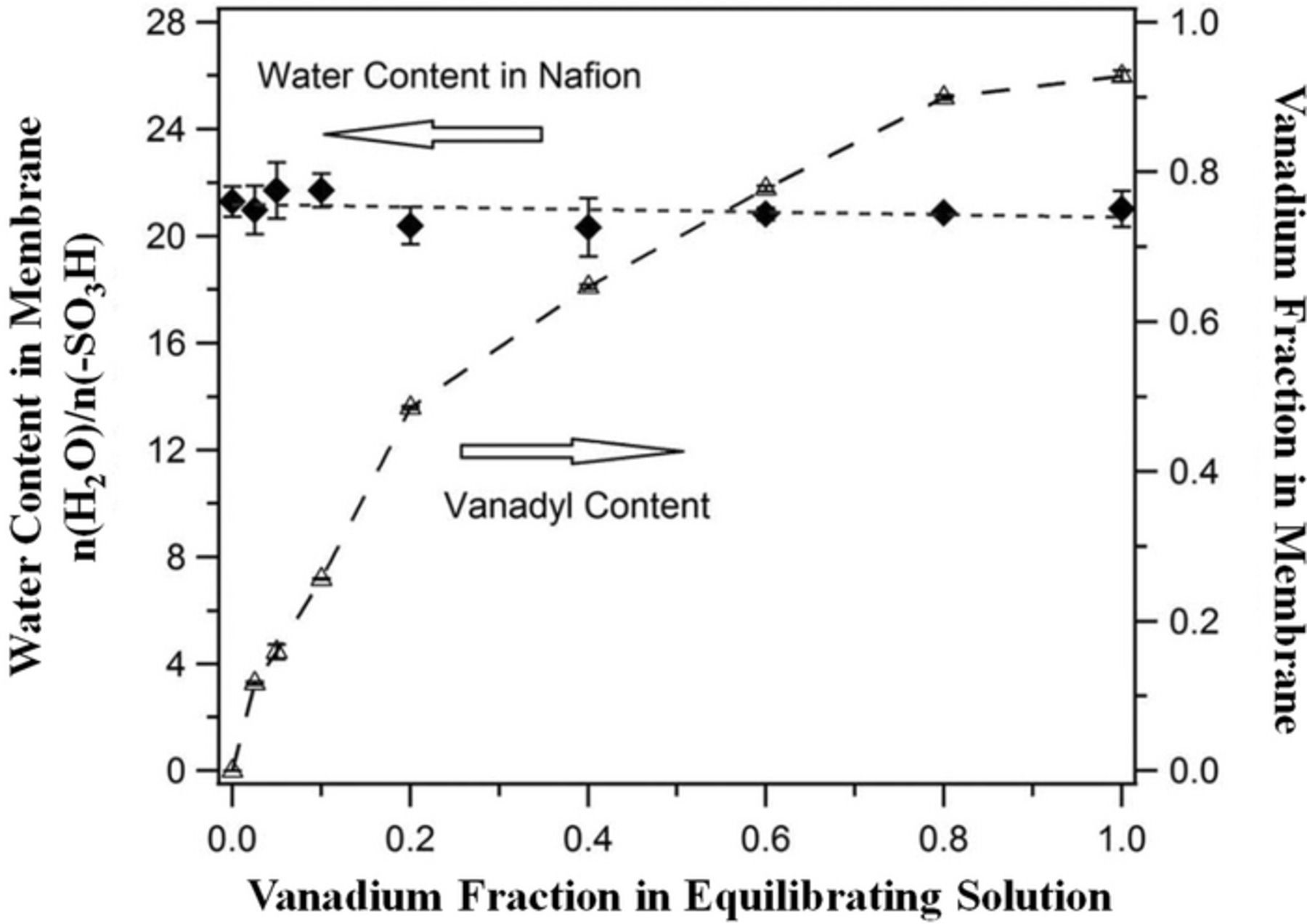
Figure 46. Water and vanadyl content in Nafion 117 equilibrated with vanadyl sulfate/sulfuric acid solutions (Ref. 233) (Note: Here, the x-axis represents vanadium fraction relative to protons and not relative to the entire solution).
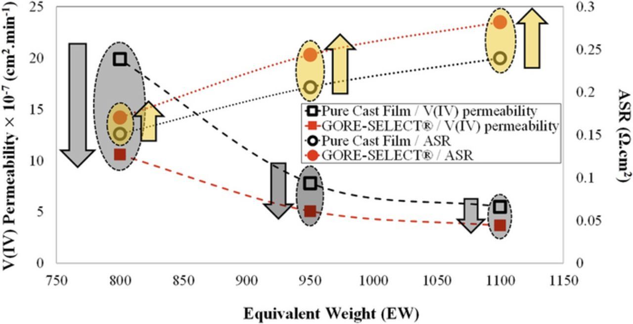
Figure 47. Correlation between equivalent weight with V(IV) permeability and ASR (Ref. 102).
Overall, the combination of Eqs. 22, 32 and 34 describes polarization behavior of an electrochemical system without explicit contributions from crossover.
Summary and Outlook
Although new chemistries are frequently introduced for RFBs, widespread commercialization is still limited due to high capital cost, low power and energy density compared to solid-state batteries, and relatively rapid capacity fade over long-term cycling. Regardless of the redox chemistry, three major goals are consistent: decreasing the material cost while boosting power and energy density to reduce overall system cost; mitigating capacity decay to maintain stable and robust performance over long-term cycling; and developing rigorous mathematical models to simulate the performance and aging behavior of the cell under different conditions.
In this review, we have discussed major available diagnostics and material characterization techniques as well as underlying governing physical phenomena used for RFBs. The diagnostics discussed are used primarily for evaluating battery cells or individual cell components and obtaining quantifiable insight into overall cell performance, and kinetic and mass transport properties, either in-situ or ex-situ. Therefore, the development of new diagnostics or improving existing diagnostics must be directed toward achieving these three major objectives.
In order to decrease overall RFB system cost, decreasing material cost and/or designing higher performance systems is required. To this end, new diagnostics must be capable of quantifying the different sources of overpotential for an operating cell and stacks with high accuracy and robustness. Increasing RFB power and energy density requires engineering cell components (e.g. minimizing sources of overvoltage including kinetics, ohmic, mass transport, and crossover) and negative/positive electrolytes (i.e. increasing the solubility and stability of electroactive species).
Investigating overpotentials
One of the most important factors in evaluating overpotential sources in an operating cell is the capability of decoupling voltage losses arising from the negative and positive half-cells. A solution to this is development of stable and robust reference electrodes, design of which likely depends on cell architecture and redox chemistry. Ideally, a reference electrode can be installed with minimal modification of cell architecture and without imposition of extra overpotential. An added obstacle to reference electrode incorporation is the need for long-term stability if used during cycling experiments.
The complexity of electron and charge transport on the surface of electrodes complicates quantifying kinetic losses in an operating cell. In order to design high-performance RFBs, it is necessary to understand electrode reaction mechanisms. Ideal redox couples must exhibit fast and reversible kinetics innately or with a low-cost, durable catalyst. For the most part, carbon-based electrodes have shown promise for various types of RFBs; however, for high power density operation, further improvement in electrochemical activity is required. New diagnostics should provide detailed information about the interfacial phenomena of the electrode/electrolyte interface which goes beyond cyclic voltammetry and impedance spectroscopy. It is necessary to better understand the details of electron transfer between the solid-phase (electrodes) and electrolyte-phase (usually liquid solution or gaseous phase) by measuring the electron transfer rate with high temporal resolution, even in real-time. Such diagnostic capabilities could also capture the processes related to electrode degradation. More importantly, for the class of RFBs utilizing catalysts, measuring the electron transfer rate and identifying the mechanism of electron transfer is necessary to identify optimal properties.
It is also necessary to decrease the ohmic overpotential for RFBs. Especially in the case of redox couples exhibiting facile kinetics or non-aqueous chemistries, ohmic losses can be quite significant. The main contributor for ohmic overpotential is typically the ion-exchange membrane's ionic resistance. Nafion has been widely used for various types of RFBs; however, cheaper and higher performance ion-exchange membranes or microporous separators must be developed. As noted, in-situ and/or ex-situ ionic conductivity measurement is common, e.g. as high frequency EIS resistance or with 4-point in-plane conductivity cells. In these techniques, conductivity is assessed at the macro-scale without providing detailed information about the ionic transport mechanism through an ion-exchange membrane; decreasing the design length scale by developing new diagnostics capable of providing more detailed information about the ion-transport mechanism can guide creation of high-performance membranes. Also, new polymers to be used as polymer backbones are frequently introduced and therefore developing diagnostics capable of capable of ascribing structure-dependent ionic conductivity is needed. New diagnostics are needed to provide further information about the effects of morphology and material treatments on ionic transport mechanisms through the membrane; such insight is valuable in addition to solely relying on the conductivity measurement. Additionally, such deeper understanding would inform degradation properties and behavior.
Reducing mass transport loss is an active area of research for various types of RFBs. The ultimate goal is to boost the local electrolyte velocity in the electrodes while minimizing parasitic pumping loss via improved flow field and electrode designs. Direct flow visualization through the porous electrodes for an operating cell would be useful; however, flow visualization is currently limited to qualitative observation using transparent flow fields and no-load conditions. Neutron imaging has been widely used for polymer electrolyte fuel cells in order to visualize two-phase flow boundaries. Conversely, for RFBs experiencing two-phase flow (i.e. visualizing gas generation as a function of side reactions), neutron imaging can be utilized for RFB study. Ultimately, understanding macro-scale transport of electrolyte through the porous media will guide optimized electrode structures. Also, the transport mechanism at a reduced length-scale (micro- and nanoscale) is not well-resolved for porous electrodes. BET, SEM, and EIS are capable of providing qualitative and quantitative information about pore structure and total and wetted surface area; however, these techniques provide information only regarding phenomena at the fiber edges with little or no detail regarding actual transport in the diffuse Nernst layer or the coupled nature of transport among the electroactive species and products.
Deeper insight regarding interactions between electroactive species in solution is required, especially for model validation. RDE is widely used for determining diffusivity values of the electroactive species in the solvent assuming infinitely dilute solution; however, these diffusivities are suspect as the electrolytes are concentrated in practice.114 Also, transport in porous electrodes is affected by pore morphology, surface energy and structure of the porous media, necessitating additional understanding.
Finally, the capability of decoupling the mechanisms of transport across porous structures and ion-exchange membranes is of great importance. In membranes, transport of electroactive species and major ionic carriers through the membranes is accomplished by diffusion, convection, and migration. Decoupling and greater molecular level understanding of those contributions via new diagnostics would be considerably helpful in identifying the most dominant mechanisms and improving properties that enhance mass transport. At the moment, only modeling simulations are capable of isolating the effect of various driving forces with no further experimental validation for each sub-division.115,116
Investigating durability and capacity fade
The second role of new diagnostics must be concentrated on providing further insight regarding capacity decay during cycling for RFBs. An ideal ion-exchange membrane must prevent this undesired transport via superior selectivity and without imposing elevated resistance toward preferred charge carriers. It may also be important to further explore and understand the effects of membrane pretreatments on the crossover-composition-structure relationship through surface spectroscopic diagnostics. In addition, degradation of cell components (i.e. electrodes and membrane fouling) is a major contributor to the capacity decay. Therefore, new diagnostics must be capable of providing structure-dependent data on the physicochemical mechanism of degradation for the cell components either in-situ or ex-situ.
Achieving rigorous and flexible models
A third role for new diagnostics is establishing the tools for validating rigorous mathematical models. Mathematical modeling along with advanced diagnostics can illuminate the fundamental phenomena controlling RFB operation and degradation. Mathematical models are maturing in three broad directions. First, improving the fidelity of the models at all scales for individual components; second, incorporating non-idealities arising from cell-level interactions; third, extending the component and cell models to include the aging behavior of systems. For all such model development, especially at micro- and nanoscales, new diagnostics must likely be developed.
At the component level, models must resolve issues surrounding multiphase flow due to the hybrid nature of some systems or when experiencing gas-generating side reactions. As a result, multiphase visualization diagnostics can be very helpful for models predicting multiphase behavior. There is a significant portion of RFBs (particularly hybrid RFBs) utilizing catalyst layers in their electrode structures. There are still issues for modeling the transport in the vicinity of catalyst layers. Particularly, the influence of a catalyst layer's properties (e.g. ionomer content, catalyst loading, porosity at the local scale which is studied in thin-film models) on the overall cell performance (at the macroscale) is not readily validated.
Finally, inclusion of component- and cell-level phenomena in stack-level models would ultimately yield a full description of an operational system. New diagnostics are required for validating the models developed for stacks. The new diagnostics can be focused on the solid/electrolyte potential distribution across multiple bipolar plates, temperature and current distribution, flow optimization/visualization within the manifold and species crossover measurement among multiple cells.
In addition, modeling the degradation behavior of an operando cell is of a great importance. One of the most important challenges is correlating the measurable properties and operation dynamics to capacity fading over time. Therefore, since degradation is a gradual process, a new set of diagnostics is required that decrease the time-scale of degradation experiments through accelerated aging. Also, at the moment, mathematical models developed for simulating the aging behavior of the RFB systems predominantly focus on altering the transport properties of the components as a function of time. However, new diagnostics must provide more in-depth understanding regarding the degradation of the cell components in real-time to correlate the observed capacity fading behavior to physiochemical changes of the components. This approach will increase the functionality of the macroscopic models for durability regardless of the chemistry used for RFB systems.
List of Symbols
| A | Projected electrode area [cm2] |
| ASR | Area specific resistance [Ω.cm2] |
| C0 | Concentration of the reacting species at the surface of an electrode [mol] |
| C*o | concentration of reactive species within the bulk solution [mol] |
| Dx | Diffusion coefficient of species x [cm2/min] |
| Ep | Working electrode potential at peak current [V] |
| E0' | Formal potential of an electrode [V] |
| f | F/RT [V−1] |
| fs | Radio frequency of the signal [Hz] |
| fref | Radio frequency of the reference signal [Hz] |
| fsp | Spectrometer radio frequency [Hz] |
| F | The Faraday constant [C] |
| i0 | Exchange current [A] |
| iK | Kinetically current density [A] |
| il | Limiting current [A] |
| ip | Peak current density [A] |
| I | Light intensity of the solute-bearing solution [cd] |
| I0 | Light intensity of a solution without the solute [cd] |
| IDchg | Cell current during discharge [A] |
| IChg | Cell current during charge [A] |
| j | Current density [A.cm−2] |
 |
Mass transport coefficient of Aα + [m.s−1] |
| k0 | Standard heterogenous rate constant [cm.s−1] |
| Ls | Distance between voltage probes [cm] |
| n | Stoichiometric number of electrons involved in the charge transfer reaction [-] |
| NElectrolytei | Flux density of species i with the electrolyte [mol.cm−2.s−1] |
| Pe | The Peclet number [-] |
| Qs | Flow rate [mL.min−1] |
| QtotalDchg | Total electrical charge withdrawn during discharging [C] |
| QtotalChg | Total electrical charge stored during charging [C] |
| R | Gas constant [J.mol−1.K−1] |
| Rs | In-plane impedance of the membrane or electrolyte [Ω] |
| Rct | Charge-transfer impedance [Ω] |
| Ss | cross-sectional area of the membrane [cm2] |
| VcellDchg | Average cell voltage during discharging [V] |
| VcellChg | Average cell voltage during charging [V] |
| v | Scan rate [V/s] |
| vc | Average flow velocity within electrode [m.s−1] |
| v0 | Velocity of the solvent [cm.s−1] |
| v* | kinematic viscosity [cm2.s−1] |
| umi | Mobility of ion (or charge carriers) i [cm2.V−1.s−1] |
| zi | Charge on species i [-] |
|
Absorbance [-] |
Greek
| α | Transfer coefficient [-] |
| ηct | Charge-transfer overpotential [V] |
| ηC | Coulombic efficiency [-] |
| ηpump | Pump efficiency [-] |
| ηV | Voltage efficiency [-] |
| λj | Wavelength at frequency j [nm] |
| σ | In-plane conductivity of the membrane or electrolyte [S.cm−1] |
| σeffs | Effective through-plane conductivity of the membrane [S.cm−1] |
| γbulkj | Activity coefficient of species j within the bulk solution |
| Φ | Solid-phase potential [V] |
| ξ | Net water drag coefficient [-] |
| ε | Porosity [-] |
| δ0 | Nernst diffusion layer thickness [cm] |
| ω | Angular frequency of rotation [s−1] |
Acknowledgments
Yasser Ashraf Gandomi acknowledge University of Tennessee for providing a Chancellors Graduate Fellowship.