Global and Local Structure of Lithium Battery Electrolytes: Origin and Onset of Highly Concentrated Electrolyte Behavior

Fabian Årén; Rasmus Andersson; Alejandro A. Franco; Patrik Johansson

doi:10.1149/1945-7111/acd8f9

Lithium-ion batteries (LIBs) are today found in mobile electronics, power tools and vehicles, and are instrumental in the electrification of the transport sector overall as well as to the renewable energy revolution. Yet further improvements in energy and power densities,¹ life-length,² and safety³ are still in high demand for LIBs. These properties are crucially dependent on the electrolyte employed; the ionic conductivities, the cation transport numbers, and the de-solvation kinetics at the electrolyte/electrode interfaces⁴ all affect the power outtake possible; the thermal, chemical and electrochemical stabilities affect the life-length and safety, etc.^5,6 Yet, the basic composition of the LIB electrolyte has changed very little in the last 25 years; it heavily relies on the PF₆ ^– anion to passivate the cathode-side Al current collector and the ethylene carbonate (EC) solvent to react to form a stable solid electrolyte interphase (SEI) on the anode side.^5,6 However, PF₆ ^– has limited thermal stability and may react to form toxic compounds,⁷ while EC has an inconveniently high melting point and viscosity which requires it to be mixed with volatile co-solvents—reducing the safety.^5,6 Today, this is kept under control by a combination of additives in the electrolyte,⁸ external safety measures, such as current interrupt devices, and by limiting the state-of-charge windows.⁹ This makes the LIBs more expensive, less flexible for the user, and more complex to build.

Alternative electrolyte concepts may overcome these shortcomings and one of the more popular routes at present is highly concentrated electrolytes (HCEs),^10–12 a concept first proposed by McKinnon and Dahn in 1985,¹³ that exhibits higher thermal stability¹⁴ and reductive^15,16 as well as oxidative¹⁷ stabilities, thus wider electrochemical stability windows (ESWs), faster intercalation kinetics¹⁸ and higher cation transport/transference numbers.^19,20 Most importantly, they do not rely on the use of the LiPF₆ salt nor are they volatile, and they may also enable lithium batteries using lithium metal anodes. Compared to the more radical approach of solid state electrolytes, which are also proposed for lithium metal anodes and to increase safety and stability,²¹ HCEs typically have higher ionic conductivities and better electrode wetting, and their greater similarities to current state-of-the-art electrolytes mean that previous R&D can be used more readily as well as current manufacturing tools and know-how applied.

The generic properties of HCEs are largely believed to be caused by their (local) structure. In a HCE none or at least a very limited concentration of "free" solvent is proposed to exist, as most should be coordinated by Li⁺ and there is a high degree of ion association; ion-pairing and higher aggregates are dominant, and all this leads to much lower volatility.¹⁴ Furthermore, it also widens the ESW by not being limited by the ESWs of the individual species.¹⁸ As these features not directly rely on particular choices of salt(s) or solvent(s), HCEs can be varied in composition to a very large extent.^10,16 The aggregated structure also opens for more complex ion transport mechanisms as vehicular transport, often assumed for conventional electrolytes, arguably should be less prominent in the highly viscous HCEs.

We have previously studied different HCEs using molecular dynamics (MD) simulation trajectories to extract structure, cation solvation shell dynamics, and transport mechanisms, etc.^22,23 Here we apply the same strategy, but we delve deeper into the specific case of LiTFSI in ACN, to study these electrolytes as function of salt concentration, focusing in on the structural properties of this transition. Unlike our previous work,^22,23 where we focused on showcasing the abilities of our new analysis method, we here use these to gain insight into the differentiating factors between conventional liquid electrolytes and HCEs, using a previously well studied HCE system. In addition, the simulation times are longer, which means we are more certain about the structures obtained,—even if no major differences are observed, and we also add more analysis, for example we study the configurational entropy as a function of concentration.

While LiTFSI in ACN electrolytes have attracted quite some interest as HCEs,^{17,18,22,24–27} one particular aim here is to explore and explain the transition from conventional electrolyte to HCE behavior for this specific case, but more importantly to try and generalize any findings to other HCEs/electrolyte chemistries as well.

Computational

AIMD simulations were performed for electrolytes consisting of LiTFSI dissolved in ACN at four different concentrations (Table I). All simulation cells were cubic, used periodic boundary conditions (PBCs), and contained 560 atoms to mitigate the effect of finite-size effects on observed trends.

Table I. Electrolyte compositions, densities, simulation cell side length and simulation lengths.

Salt:solvent molar ratio	Salt concentration [M]	#LiTFSI	#ACN	Density^{^a)} [g cm⁻³]	a [Å]	Equilibration run time [ps]	Production run time [ps]
1:16	1.0	5	80	0.968	20.08	0.83	30.0
1:9	1.6	8	72	1.08	20.06	0.98	3.8
1:4	2.9	14	56	1.29	20.11	0.91	4.0
1:2	4.0	20	40	1.48	20.24	0.95	34.4

^a)Dr. Viktor Nilsson, Chalmers, personal communication 2020.

All the above used the NVT ensemble at 293 K and a Nosé-Hoover thermostat^28,29 with ω_ions = 2250 cm⁻¹ and ω_electrons = 4500 cm⁻¹ within the Car-Parrinello MD (CPMD)³⁰ software and the Perdew–Burke–Ernzerhof (PBE)³¹ functional, with a plane wave cut-off of 70 Ry and a fixed time step of 0.1 fs. The time needed for equilibration was found by considering the decay of the sum of pointwise squared errors of all partial radial distributions functions (pRDFs) compared with their time average, as in previous studies.^22,23 While this timescale is not necessarily long enough to equilibrate the systems fully, it is sufficient for each ion and molecule to find its local minimum w.r.t. orientation and next neighbor distances, and for unreasonably large local stresses to be relaxed. The least and most concentrated electrolytes were therefore run for much longer, and reassuringly their local behavior remained consistent. The initial geometries were generated by randomizing and relaxing the positions and orientations of ions and molecules, by a conjugate gradient descent method w.r.t. a cost function designed to avoid overlap of atoms.³² The TFSI anions were initialized as 50% cis and 50% trans conformations³³ and pre-optimized using the Gaussian 16 software³⁴ at the M06–2X/6–311+G(d,p) level of theory.³⁵

From the AIMD simulation trajectories all covalent and coordination bonds were subsequently identified using CHAMPION (Chalmers Atomic, Molecular, Polymeric & Ionic analysis toolkit).^22,32 A time-dependent bond graph was constructed for each simulated system where the global structure is characterized by connected components and the local environments of Li⁺ ions by their 1st solvation shells. The distinct types of components and solvation shells are classified by their subgraph topologies, which are treated statistically to enable analysis of their structures. The size distributions of connected components are quantified in terms of the probability mass functions (PMFs) for the number of each species (Li⁺, TFSI, ACN) in a connected component, where PMF(n) denotes the probability of exactly n exemplars, and also their integrals, the cumulative distributions functions (CDFs), where CDF(n) is the probability of having up to n exemplars. For a more thorough description of how these algorithms are constructed and implemented in CHAMPION we refer to our previous papers.^22,32,36

The above enables a detailed analysis of the global structure as well as the cation 1st solvation shell composition including the Li⁺ (partial) solvation numbers (SNs) and coordination numbers (CNs). The partial CN (pCN) of each Li⁺-coordinated species (ACN and TFSI) is its number of coordination bonds to a Li⁺ ion and the total CN is the sum of these contributions, whereas the partial SN is the number of distinct exemplars of each species in the 1st solvation shell and the total SN likewise is the sum of pSNs.

Lastly, we calculate the configurational entropy of each system using Gibbs entropy formula:

$\begin{eqnarray*}&&{S}_{G}=-{k}_{B}\displaystyle \sum {p}_{i}\,\mathrm{log}\,{p}_{i}\end{eqnarray*}$

where p_i is the frequency probability of a dynamically bonded structure i, identified through CHAMPION, with the assumption that all are homogeneously dispersed throughout the simulation box.

Results and Discussion

Starting with the global structure, by considering the size distributions and compositions of connected components and the fraction of free solvent molecules and anions, as well as representative simulation snapshots, we subsequently turn to uniquely assess the local structure looking primarily at Li⁺ 1st solvation shell structures. Finally, to complement the insights gained from studying the local structure, the configurational entropy of each system is calculated from the identified structures. By doing all of this for the four differently concentrated electrolytes a unified picture of differences and similarities is created, also highlighting the origin of and the transitions to HCE behavior.

Global structure

We first assess the overall global structure of the electrolytes by evaluating the PMFs (Figs. 1a–1c) and CDFs (Figs. 1d–1f) of Li⁺ to be in components with different number of cations, solvent molecules, and anions. Starting with the two least concentrated electrolytes (1:16 and 1:9) the Li⁺ and ACN distributions (Figs. 1a–1b, 1d–1e) are close to identical, which can be inferred to a local coordination where pSN_ACN and pCN_ACN, both equal to four, i.e. [Li(ACN)₄]⁺, is very dominant. The main difference is found for the TFSI distribution (Figs. 1c, 1f); in 1:16 ∼70% of the components contain no TFSI ions as compared to ∼40% in the 1:9 electrolyte. For both electrolytes there are smaller peaks for two TFSI ions with probabilities of ∼25%, and even fewer components with a single TFSI ion, and practically no components with three or more TFSI ions. Hence these two electrolytes do not adhere structurally to what conventionally defines HCEs as they lack extensive ion-ion aggregation, even though for 1:9 ca. two-thirds of the Li⁺ ions are connected with TFSI anions in some way.

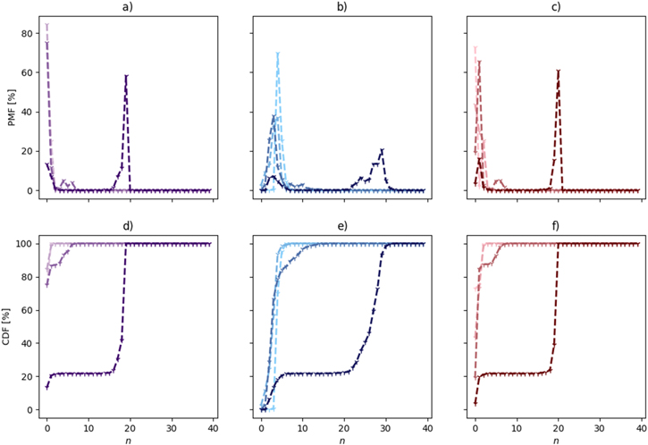
**Figure 1.** PMFs and CDFs of species in Li⁺ containing connected components: (a), (d) Li⁺; (b), (e) ACN; and (c), (f) TFSI. The electrolyte concentrations are visualized by lightest (1:16) to darkest shade (1:2).
Download figure:
Standard image High-resolution image

For the 1:4 electrolyte a broad peak appears around 5–7 li⁺ ions in the PDF (Fig. 1a), with corresponding peaks at 10 ACN (Figs. 1b and 5–6 TFSI (Fig. 1c), while for the 1:2 electrolyte the PMFs are close to involving all ions and an even larger number of solvent molecules. This corroborates that the 1:2 electrolyte forms a percolating network, but also that it is just above the percolation threshold (as the 1:4 electrolyte does not form one).²²

The overall trends of the global structure are perhaps most clearly visible using the CDFs (Figs. 1d–1f) where the two less concentrated electrolytes contain only single ions, ion-pairs and small aggregates, whereas the intermediate concentrated electrolyte exhibits also intermediate sized clusters of typically ca. 5 salt units and 9 ACN molecules, and the most concentrated electrolyte is totally dominated by the percolation giant component containing almost 90% of the ions and in addition also half of the solvent molecules.

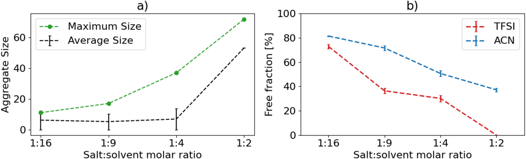
The trend in the average total number of species per component (Fig. 2a), showing the leap between 1:4 and 1:2, gives an even better representation of the percolation network formation. The trends for the fractions of free solvents and anions (Fig. 2b) show the former to be roughly halved, from 80% to 40%, whereas the latter goes from 70% down to 0. The decrease in free ACN fraction is almost linear with respect to concentration.

**Figure 2.** (a) Average and maximum aggregate size in number of total ions and solvent molecules in connected components, and (b) fraction of free, i.e. uncoordinated to Li⁺, anions and solvent molecules, as functions of electrolyte salt concentration. (For 1:2 too few data points become available to make an error-bar sensible in (a)).
Download figure:
Standard image High-resolution image

The trends overall agree well with the literature (Fig. S2). For the three less concentrated electrolytes, the fraction of free ACN is very close to the average of previously reported results from both Raman spectroscopy and classical MD studies.^18,24,25 For the 1:2 electrolyte and as compared to Raman data, our fraction of 40% is somewhat greater than the ca. 33% reported by Brouillette et al.²⁴ and in particular the ca. 11% reported by Seo et al.,²⁵ albeit the latter used quite a bit higher temperature (60 °C). The overall appearance of the data is, however, remarkably similar, especially to that of Brouillette et al.²⁴ Yamada et al.¹⁸ also presented room temperature Raman data, and while they did not explicitly compare peak areas, their data indicate the free ACN fraction to go from very large at 1.0 M to almost non-existent at 4.2 M. The MD simulation data of Seo et al.²⁵ agree well with their Raman data, but with a more steady linear decrease as function of salt concentration.

With respect to the free TFSI fraction, our results are broadly in line with previously reported results, which are, however, much more ambiguous than those for ACN (Fig. S2).^18,24,25 This is most likely due to the difficulty of distinguishing contact ion pairs from free anions by Raman spectroscopy.³⁷ Our free TFSI fraction is lower than reported by Brouillette et al.²⁴ and Seo et al.,²⁵ but in line with Yamada et al.¹⁸ At the same time, it is higher than those obtained from MD simulations.²⁵

While we obtain a slightly higher fraction of free solvent for the 1:2 electrolyte than previously reported, the preponderance of evidence speaks for free ACN not being entirely eliminated at this concentration. This calls into question the explanation commonly given both for the low volatility and especially for the widened ESWs of HCEs, i.e. no free solvent remaining.¹⁸ The latter points to cation-anion interactions shifting the electronic levels of the anions potentially being more important than cation-solvent interactions and the corresponding changes in the solvent molecules at room temperature. Alternatively, the effect is mainly kinetic, constraining the motion of the free ACN, rather than energetic. However, we should keep in mind that the HCE structure at and close to the electrolyte/electrode interface could be quite different than in the bulk and the possible need for longer equilibration than available from the AIMD simulations.

Snapshots from the MD simulation trajectories can anyhow provide a more intuitive view of the overall structural changes as function of concentration (Fig. 3). For the 1:16 electrolyte most Li⁺ ions are in [Li(ACN)₄]⁺ solvates, but there is also an example of an aggregate of two Li⁺ ions, two TFSI ions and five ACN solvent molecules. For the 1:9 electrolyte basically the balance between these two features can be seen to change, while for the 1:4 electrolyte the beginnings of a network structure can be seen, though it never percolates throughout until the 1:2 electrolyte; in the snapshot shown this indeed involves all ions. This agrees well with the network structure illustrated by Yamada et al. from their AIMD simulations.¹⁸

**Figure 3.** Snapshots of MD simulation trajectories for the four electrolytes. The boxes represent the PBCs and only one image of each atom is displayed.
Download figure:
Standard image High-resolution image

Local structure

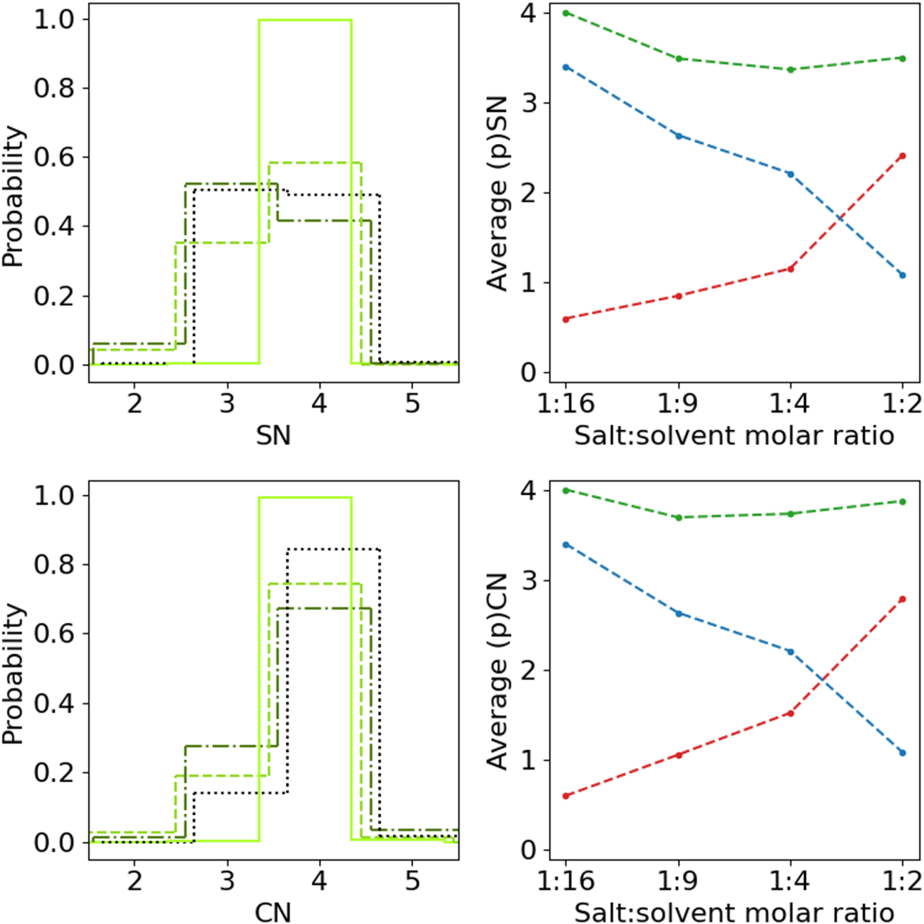
Moving on to the local structure and the Li⁺ 1st solvation shells, we first consider the SN distributions (Fig. 4a). Also here there is a clear difference between the two less concentrated electrolytes on the one hand and the intermediate and most concentrated electrolytes on the other. The former two are completely dominated by SN = 4, as could be expected from the global structure, while the latter two have their maxima for SN = 3, which is less obvious from the global structure data. The overall trend is that each observed increase in concentration results in an increase in the probability of SN = 3 at the expense of SN = 4. Considering instead the average pSNs of TFSI and ACN, as well as the average SN (Fig. 4b), moving from 1:16 via 1:9 and further to 1:4, there is a steady decrease in solvation by ACN and a slightly less steep concomitant increase in TFSI interaction, both of which become steeper in the step to 1:2. This results overall in a minor decrease in the average SN as function of salt concentration from 4.0 for 1:16 to 3.8 for 1:2.

**Figure 4.** (a), (c) SN and CN distributions from 1:16 (light, solid) to 1:2 (dark, dotted) and (b), (d) average pSN and pCN for ACN (blue) and TFSI (red), and SN and CN (green), respectively, as function of electrolyte salt concentration.
Download figure:
Standard image High-resolution image

The CN distributions (Fig. 4c) contrast with the SN distributions dominated by CN = 4 for all four concentrations, with different smaller contributions from CN = 3 and negligible contributions from all other CNs. The two most concentrated electrolytes both have larger contributions from CN = 3, with the 1:4 concentration having a larger contribution than the 1:2 concentration. This can be explained by the substantially longer simulation time for the 1:2 system, indicating that the 1:4 system could probably evolve toward a smaller but not insignificant CN = 3. The least concentrated electrolyte (1:16 ) have a smaller contributions from CN = 3 with 1:9 having a similarly artificially high CN = 3 as 1:4. The average (p)CNs and (p)SNs reported here agree quite well the literature,²⁵ especially with respect to ACN, but data reported by Seo et al. has no slight decrease in average SN with increasing salt concentration (Fig. S3).

Considering the full distributions of pSN_ACN and pSN_TFSI, neither is practically ever >4 (Fig. 5). pSN_ACN is distributed between 2 and 4 for 1:16, with pSN_ACN = 4 being the largest contribution. For 1:9 the distribution broadens as the probability mass down-shifts, to include also pSN_ACN = 1. This broadening and down-shift continues, moving the maximum to 3 for 1:4, and 1 for 1:2. For the most concentrated electrolyte, pSN_ACN = 4, and thus [Li(ACN)₄]⁺, is virtually eliminated, and a third of the Li⁺ 1st solvation shells have no ACN at all. For the pSN_TFSI the trend is almost the opposite; for the 1:16 electrolyte most Li⁺ ions coordinate to 0 TFSI ions with substantially lower probability for 1 and 2, while for the 1:9 electrolyte the probability is almost evenly distributed among 0–2., with pSN_TFSI = 2 being slightly lower than the other two. For 1:4, pSN_TFSI = 1 dominates, accounting for more than half the probability mass, as does pSN_TFSI = 3 for 1:2.

**Figure 5.** pSN_ACN (blue) and pSN_TFSI (red) for the four electrolytes.
Download figure:
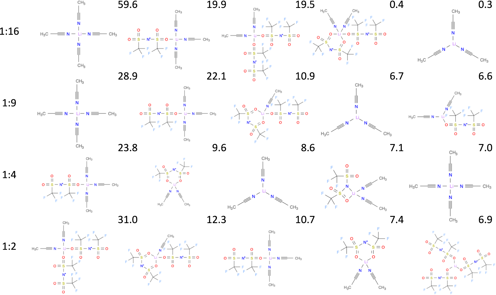
Standard image High-resolution image

Finally, when we consider the five most common 1st solvation shell structures for each of the electrolytes, the structural diversity in general increases as a function of salt concentration (Fig. 6, i.e. decreased probability for the most common structures, which is consistent with variations in the local HCE structure reported by Åvall et al.^39,40 In more detail, ACN is always monodentately coordinated to Li⁺ by the nitrogen of the nitrile group, while TFSI exhibits a much more varied coordination to Li⁺: bidentately by two sulfonyl oxygen atoms or with one of them replaced by the central nitrogen atom, but the much more common coordination is monodentately by a single sulfonyl oxygen atom. Both these types of coordination agree well with the LiTFSI structures found by Henderson et al.⁴¹

**Figure 6.** The topologies and percentage fraction of the five most common local structures for the four electrolytes rendered as structural diagrams.³⁸
Download figure:
Standard image High-resolution image

It is also quite clear that the Li⁺ ion local structures semi-quantitatively are very similar for the two less concentrated electrolytes, especially as the most common structure, [Li(ACN)₄]⁺, is the same, and three out of five possible structures are among the top five for both electrolytes, i.e. additionally Li(TFSI)(ACN)_3, and [Li(ACN)₃]⁺. The differences between them also explicates the view given above; 1:9 has more interacting TFSI ions with the third most common structure having bidentate coordination, whereas 1:16 has only monodentate coordination, besides 0.4% bidentate coordination, among the top five structures and has 0.3% [Li(ACN)₃]⁺, compared to 6.7% for 1:9. For the two more concentrated electrolytes [Li(ACN)₄]⁺ is no longer amongst the five most common structures for 1:2, and barely makes it into the top five for 1:4, but [Li(ACN)₃]⁺ is, however, the third most common structure for the 1:4 electrolyte, likely due to a fourth ACN often not being available, as discussed above, while also this structure is relegated beyond top five for 1:2. For the 1:2 electrolyte the most common local structures all include more than one coordination bond to TFSI, which dominates the 1st solvation shell, which agrees well with the observations made by Kameda et al.⁴² that for their (LiTFSI)(ACN)₂ electrolyte, studied by neutron diffraction, show that Li coordinates with 1.63 ± 0.07 ACN molecules and 2.0 ± 0.1 TFSI ions.

Notably the fifth most common structure, making up over 6%, exclusively consist of three TFSI ions - which largely explains the pSN_ACN = 0 feature (Fig. 5). Connecting further to the data in Fig. 5, the pSN_ACN = 2 feature for the 1:2 electrolyte is also indicated here, as the most common local structure have two ACN solvent molecules in the Li⁺ 1st solvation shell. While the top structures for 1:2 were also reported in our previous work²² and were based on the same simulation trajectories, the CHAMPION code base has since then undergone some major modifications, but only minor modifications to the underlying algorithms and the parameters controlling tolerances and sensitivities in CHAMPION, primarily affecting the bidentate coordination have been made, which nevertheless changes the exact ordering of the structures.

Configurational entropy

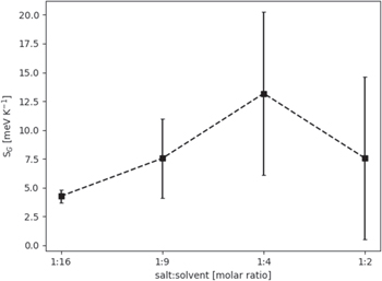
Finally, looking at the full ensemble of structures, the configurational entropy, based on the speciation and connectivity—thus reflecting both global and local structure, shows a clear drop from 1:4 and 1:2, after having steadily increased from 1:16 to 1:4 (Fig. 7). We again attribute this to the percolating network formed, which makes the system more ordered. Similar claims have recently been made in the electrolyte literature.^43,44 The error-bars increase as a function of concentration, when more of the ions and molecules exist within the same structure, this heavily reduces the number of data and worsen the statistics. Comparing with literature⁴⁵ our measure of configurational entropy is on the same order of magnitude as the standard molar entropy of 1 M LiTFSI in ACN. However, no direct comparison should be made between these measures since our measure of configurational entropy is only one contributing factor in the standard molar entropy.

**Figure 7.** Configurational entropy as a function of electrolyte salt concentration.
Download figure:
Standard image High-resolution image

Concluding Remarks

The research interest in HCEs largely originates in the many macroscopically manifested attractive properties. While some of these arguably are highly surface/interface/interphase dependent, studying the bulk electrolyte is anyhow a good starting point for an overall understanding of HCEs. Lack of free solvent is often argued as a key feature, but even for very concentrated electrolytes we find a substantial fraction of uncoordinated solvent present, albeit perhaps not enough to render them conventional electrolyte bulk properties.

The overall picture emerging is rather composed of several different features, all of which are important to different extent. At salt concentrations close to the conventional, 1 M, (1:16) 50% of the ions are free and the rest are found in ion-pairs and small aggregates. The latter two local structures increase with salt concentration until, at ca. 3 M (1:4), the aggregates increase in size and eventually form a percolating network between 3 and 4 M. The network involves almost all ions, but not all solvent molecules, which on the other hand do not form a continuous phase. How well this generalizes to other HCEs is largely open for discussion. We can for example foresee that for a stronger coordinating or even a polydentate solvent, instead of the weakly coordinating monodentate ACN solvent used here, a network could more easily form that is made up of a mixture of solvent, anions, and cations, and the nature of the main moving species will accordingly be able to change drastically. On the other hand we do believe that, given the use of "standard" HCE salts the balance between cation-anion and ion-solvent interactions will remain more or less the same, as the pair-wise ion-solvent interactions will always be much weaker than cation-anion interactions. Thus, the changes observed may mainly be the on-set salt concentration of percolation network formation. However, all of the above is speculative and of course calls for validation—we do not know (yet) if and how percolation networks in general affect the properties of HCEs. All of this, with respect to presence and state of the solvent, has implications for the safety aspect of HCEs. Overall, a greater nuance is warranted in terms of how HCEs are in general defined and understood—here we find most of the salient transitions to coincide with the formation of the percolating network, making this the best candidate for what distinguishes HCE structure and behavior, rather than the often mentioned elimination of free solvent.

Finally, some caution is warranted due to the limited timescales and system sizes used. Ideally, classical MD simulations with well validated force fields should be applied to ensure both proper equilibration and better statistics. Still, much can be learnt conceptually about the local structure of electrolytes from the rather modest simulation lengths and system sizes applied herein, and any full multi-scale understanding of electrolytes must start from an accurate description on the level of ions and molecules.

Acknowledgments

The research presented has received funding through the HELIS project (European Union's Horizon 2020 research and innovation program under Grant Agreement No. 666221) and the Swedish Energy Agency grants (#P43525–1 and #P39909–1). P.J. would also like to acknowledge the BASE network as well as Chalmers Areas of Advance Materials Science and Energy, for continuous support, and specifically the Theory and Modelling scheme of Advanced User Support to F.Å. and R.A. A.A.F. acknowledges the Institut Universitaire de France for the support.

F.Å., R.A. and P.J. are shareholders of Compular AB, the company developing CHAMPION.

Global and Local Structure of Lithium Battery Electrolytes: Origin and Onset of Highly Concentrated Electrolyte Behavior

Article metrics

Author e-mails

Author affiliations

ORCID iDs

Dates

Abstract

Computational