Constraints on Higgs boson properties using $WW^{*}(\rightarrow e\nu \mu \nu )jj$ production in $36.1\,\mathrm{fb}^{-1}$ of $\sqrt{s}=13$ TeV pp collisions with the ATLAS detector

Abstract

This article presents the results of two studies of Higgs boson properties using the $WW^*(\rightarrow e\nu \mu \nu )jj$ final state, based on a dataset corresponding to ${36.1}{{\mathrm{fb}}^{-1}}$ of $\sqrt{s}=13$ TeV proton–proton collisions recorded by the ATLAS experiment at the Large Hadron Collider. The first study targets Higgs boson production via gluon–gluon fusion and constrains the CP properties of the effective Higgs–gluon interaction. Using angular distributions and the overall rate, a value of $\tan (\alpha ) = 0.0 \pm 0.4 (\mathrm {stat.}) \pm 0.3 (\mathrm {syst.})$ is obtained for the tangent of the mixing angle for CP-even and CP-odd contributions. The second study exploits the vector-boson fusion production mechanism to probe the Higgs boson couplings to longitudinally and transversely polarised W and Z bosons in both the production and the decay of the Higgs boson; these couplings have not been directly constrained previously. The polarisation-dependent coupling-strength scale factors are defined as the ratios of the measured polarisation-dependent coupling strengths to those predicted by the Standard Model, and are determined using rate and kinematic information to be $a_\mathrm {L}=0.91^{+0.10}_{-0.18}$(stat.)$^{+0.09}_{-0.17}$(syst.) and $a_{\mathrm {T}}=1.2 \pm 0.4$(stat.)$^{+0.2}_{-0.3}$(syst.). These coupling strengths are translated into pseudo-observables, resulting in $\kappa _{VV}= 0.91^{+0.10}_{-0.18}$(stat.)$^{+0.09}_{-0.17}$(syst.) and $\epsilon _{VV} =0.13^{+0.28}_{-0.20}$ (stat.)$^{+0.08}_{-0.10}$(syst.). All results are consistent with the Standard Model predictions.

1 Introduction

The Higgs boson (H) discovery at the Large Hadron Collider (LHC) was a great success of the ATLAS and CMS Collaborations [1, 2]. Since the discovery, multiple studies have been performed to establish whether the Higgs boson has the properties predicted by the Standard Model (SM), or instead is a particle of an as yet unobserved sector beyond the SM. The mass of the Higgs boson has been measured by the ATLAS and CMS experiments to be $m_H = 125.09 \pm 0.21(\mathrm {stat.})\pm 0.11 (\mathrm {syst.}) \;\text {GeV}$ [3] using $\sqrt{s}=7$ and $8\;\text {TeV}$ pp collision data, and there are strong indications that the spin and parity states are $J^{P}=0^{+}$ [4,5,6]. By probing the final-state particles in $H\rightarrow WW^{*}$, $H\rightarrow ZZ^{*}$, and $H\rightarrow \gamma \gamma$ decays, a pure CP-odd Higgs boson has been excluded at a confidence level above $99.9\%$. In addition, a potential CP-odd contribution to the HWW and HZZ couplings has been significantly constrained [7,8,9]. Recently, studies of the CP properties of the top-quark Yukawa coupling using Htt events, and the $\tau$-lepton Yukawa coupling using $H\rightarrow \tau \tau$ decays have been published [10,11,12].

The gluon–gluon fusion ($\mathrm {ggF}$) process probes a different kinematic regime than Htt production, and the properties of the effective ggH interaction itself may differ from SM predictions if there is a loop contribution from previously unobserved particles. The CP nature of the effective coupling between the Higgs boson and gluons, ggH, in the gluon–gluon fusion production mode [13] has been studied in Refs. [14,15,16]. This article presents new analysis techniques for enhancing the sensitivity to interference effects between the CP-even and CP-odd contributions to the Higgs–gluon coupling, and provides constraints on the mixing angle between CP-even and CP-odd contributions. The approach is therefore complementary to those used in previous studies of the CP properties of the Higgs boson.

Fig. 1

Examples of Feynman diagrams contributing to the production of a Higgs boson in association with two jets via the fusion of two gluons or two vector bosons (V) at leading order in QCD. The presented diagrams show examples for the subprocesses a $qq\rightarrow H qq$, b $qg\rightarrow H qg$ and c $gg\rightarrow H gg$, as well as d the vector-boson fusion process and the subsequent decay of the Higgs boson into two vector bosons

The vector-boson fusion (VBF) Higgs boson production process has been measured by ATLAS and CMS in numerous channels [7, 8, 17,18,19,20]. While measurements of $\sigma _\mathrm {VBF} \cdot {\mathcal {B}}_{H\rightarrow WW}$ are consistent with the SM, individual polarisation-dependent Higgs boson couplings to the massive electroweak gauge bosons have so far not been studied directly. Longitudinally polarised electroweak bosons emerge from massless degrees of freedom of the Higgs boson and are therefore closely related to the mechanism of electroweak symmetry breaking. The strength of the Higgs boson coupling to longitudinally polarised W bosons ensures the unitarity of the SM. However, if the Higgs field is not associated with a fundamental scalar particle but is an effective field arising from new dynamics, the coupling may deviate from its SM value. For example, Higgs compositeness models [21, 22] predict more degrees of freedom, allowing the Higgs boson couplings to electroweak bosons to deviate from their SM values.

This article presents the results of two analyses studying the properties of the Higgs boson using its decay into $WW^{*}\rightarrow e\nu \mu \nu$ and its production in association with two jets (jj). The first analysis targets gluon–gluon fusion Higgs boson production and is sensitive to the CP properties of the ggH effective coupling and the top-quark Yukawa coupling. The second analysis constrains Higgs boson couplings to longitudinally and transversely polarised W and Z bosons in the VBF production mode, assuming a CP-even Higgs boson. Both studies are based on proton-proton collision data corresponding to an integrated luminosity of $36.1\;\mathrm {fb}^{-1}$ collected with the ATLAS detector at $\sqrt{s} = 13~\text {TeV}$ in the years 2015 and 2016. Representative leading-order diagrams for the $\mathrm {ggF}$ + 2 jets and VBF production modes are depicted in Fig. 1a–c and d, respectively.

Both analyses use the shape of the signed azimuthal angle¹ difference $\Delta \Phi _{jj}$ between the two leading hadronic jets in the selected $H + 2$-jets candidate events to test for deviations from the SM expectations. The angular difference is defined as $\Delta \Phi _{jj}=\phi _{j_1} - \phi _{j_2}$ if $\eta _{j_1} > \eta _{j_2}$, and $\Delta \Phi _{jj}=\phi _{j_2} - \phi _{j_1}$ otherwise, where $j_1$ is the highest-$p_\mathrm {T}$ jet and $j_2$ is the next-highest-$p_\mathrm {T}$ jet in the event. The distribution of $\Delta \Phi _{jj}$ is probed in various disjoint kinematic regions, optimised for each analysis specifically.

The structure of this article is as follows. Section 2 gives a short summary of the theoretical frameworks used to study the CP properties of the Higgs boson’s coupling to top quarks and gluons, as well as its coupling to polarised electroweak bosons. The ATLAS detector and the Monte Carlo and data samples used in these studies are discussed in Sects. 3 and 4, respectively. The event selection and categorisation requirements are presented in Sect. 5, while the estimation of the various background processes is detailed in Sect. 6. The theoretical and experimental uncertainties are presented in Sect. 7. Finally, the results are discussed in Sect. 8.

2 Theoretical framework and methodology

For the studies targeting beyond-the-SM (BSM) contributions to the top-quark Yukawa coupling and the effective Higgs–gluon coupling, an effective field theory (EFT) framework is chosen to parameterise possible deviations from the SM. The EFT operators probed in this article are provided by the Higgs Characterisation (HC) model [23], which is implemented in the MadGraph5_aMC@NLO generator [24, 25]. In the large top-quark-mass limit, $m_\mathrm {top}\rightarrow \infty$, the CP structure of the top-quark Yukawa coupling is inherited by the effective Higgs–gluon interaction [26]. Thus, constraints on BSM contributions will be directly set on the CP-even and CP-odd coupling strength modifiers of the effective Higgs–gluon interaction. The effective Lagrangian that describes the Higgs–gluon interaction is expressed as

$$\begin{aligned} \qquad \quad {\mathcal {L}}^\mathrm {loop}_{0}= & {} -\frac{g^{}_{Hgg}}{4}\left( \kappa ^{}_{gg} \cos (\alpha ) G^a_{\mu \nu }G^{a,\mu \nu } \right. \nonumber \\&\qquad \quad \left. + \kappa ^{}_{gg} \sin (\alpha ) G^a_{\mu \nu }{\tilde{G}}^{a,\mu \nu }\right) H, \end{aligned}$$

(1)

Table 1 Definition of the three benchmark scenarios used in the $\mathrm {ggF}$ + 2 jets analysis. The parameter settings correspond to a CP-even (i.e. the SM hypothesis), a CP-odd, and a CP-mixed scenario

Fig. 2

Distributions of the signed $\Delta \Phi _{jj}$ observable shown for a CP-even, CP-odd and CP-mixed benchmark models of the $\mathrm {ggF}$ + 2 jets production mode, and b various configurations of the $a_\mathrm {L}$ and $a_\mathrm {T}$ parameters in VBF events. These comparisons are performed at the generator level using the predictions of the MadGraph5_aMC@NLO 2.4.2 + Pythia 8.212 [32] generators

where $G^a_{\mu \nu }$ is the gluon field strength tensor, ${\tilde{G}}^{a,\mu \nu }= G^a_{\rho \sigma }\,\varepsilon ^{\mu \nu \rho \sigma }/2$ is the dual tensor, $g^{}_{Hgg}$ is the effective coupling for the SM CP-even ggH interaction, $\kappa ^{}_{gg}$ is the coupling-strength scale factor for the effective Higgs–gluon interaction and $\alpha$ is the CP-mixing angle. Interference between CP-even and CP-odd contributions affects the shape of the signed $\Delta \Phi _{jj}$ distribution, but has no impact on the cross section of the $\mathrm {ggF}$ production mode, which is a function of $\kappa _{gg}^2\cos ^2(\alpha )$ and $\kappa _{gg}^2 \sin ^2(\alpha )$ only. Three benchmark scenarios with different CP properties are defined in Table 1, and the distribution of the signed $\Delta \Phi _{jj}$ observable is shown in Fig. 2a for these parameter choices.

The analysis targeting HVV couplings in Higgs boson production and decay uses polarisation-dependent coupling-strength scale factors defined in Ref. [27] as

$$\begin{aligned}&\displaystyle a_\mathrm {L} = \frac{g_{HV_\mathrm {L}V_\mathrm {L}}}{g_{HVV}}\,, \; a_\mathrm {T} = \frac{g_{HV_\mathrm {T}V_\mathrm {T}}}{g_{HVV}}\, ,&\end{aligned}$$

(2)

where $g_{HVV}$ is the SM HVV coupling strength and $g_{HV_\mathrm {L}V_\mathrm {L}}$ and $g_{HV_\mathrm {T}V_\mathrm {T}}$ are the measured polarisation-dependent couplings.

The polarisations of the vector bosons in Eq. (2) are defined in the Higgs boson rest frame so that mixed-polarisation couplings $HV_\mathrm {L}V_\mathrm {T}$ do not contribute to $\sigma _\mathrm {VBF} \cdot {\mathcal {B}}_{H\rightarrow WW}$. Other BSM effects are not considered. Within the SM ($a_\mathrm {L}=a_\mathrm {T}=1$), the HVV couplings are insensitive to the polarisations.

Since the polarisations depend on the measurement frame, the above description is not Lorentz invariant and as such cannot be described in the Lagrangian framework. Instead, the coupling strength modifiers $a_\mathrm {L}$ and $a_\mathrm {T}$ can be related to pseudo-observables (POs) [28]. The POs considered in this article appear as $\kappa _{VV}$ and $\varepsilon _{VV}$ in the effective Lagrangian

$$\begin{aligned} {\mathcal {L}}= & {} \kappa _{VV} \left( \frac{2m_{W}^2}{v} H W^{+}_\mu W^{-\mu } + \frac{m_{Z}^2}{v} H Z_\mu Z^\mu \right) \\&\quad - \frac{\varepsilon _{VV}}{2v} \left( 2HW^+_{\mu \nu } W^{-\mu \nu } + HZ_{\mu \nu } Z^{\mu \nu } + HA_{\mu \nu } A^{\mu \nu } \right) \,, \end{aligned}$$

where in the SM $\kappa _{VV}=1$ and $\varepsilon _{VV}=0$. The universality of Higgs boson interactions with longitudinal W and Z bosons follows from assuming custodial symmetry (see Eqs. (33) and (35) in Ref. [29]), no new physics in the boson–fermion couplings Wff and Zff, and a CP-even Higgs boson with CP-conserving interactions with vector bosons. Since the study does not probe $HZ\gamma$ and $H\gamma \gamma$ interactions, for simplicity a common coupling factor is assumed for Higgs-boson interactions with transversely polarised W and Z bosons, and photons.

The POs are related to the coupling-strength scale factors $a_\mathrm {L}$ and $a_\mathrm {T}$ via the following equations:

$$\begin{aligned} \kappa _{VV}= & {} a_\mathrm {L} - \Delta _\mathrm {L}(q_1, q_2) \varepsilon _{VV}\,, \\ \varepsilon _{VV}= & {} \frac{a_\mathrm {T} - a_\mathrm {L}}{\Delta _\mathrm {T}(q_1, q_2)- \Delta _\mathrm {L}(q_1, q_2)} \,. \end{aligned}$$

The functions $\Delta _\mathrm {L}(q_1, q_2)$ and $\Delta _\mathrm {T}(q_1, q_2)$ depend on the momenta of electroweak bosons $q_{1}$ and $q_{2}$ (either in the production or in the decay) according to:

$$\begin{aligned} \Delta _\mathrm {L}= & {} \frac{m_H^2}{2 m_W^2} \frac{4q_1^2 q_2^2}{m_H^2(m_H^2 -q_1^2 -q_2^2)}\,, \\ \Delta _\mathrm {T}= & {} \frac{m_H^2}{2 m_W^2}\frac{m_H^2 -q_1^2 -q_2^2}{m_H^2}\,. \end{aligned}$$

Based on the simulations of the VBF signal discussed in Sect. 4, $\Delta _\mathrm {L}(q_1, q_2)=0$ and $\Delta _\mathrm {T}(q_1, q_2)=2$ are found to be good approximations, leading to the mapping

$$\begin{aligned} \kappa _{VV} \simeq a_\mathrm {L}\,, \quad \varepsilon _{VV} \simeq 0.5\cdot (a_\mathrm {T} - a_\mathrm {L})\,. \end{aligned}$$

The above POs description focusses on VBF production and thus differs from the one used in Refs. [30, 31], in which couplings to leptons ($\varepsilon _{L}$, $\varepsilon _{R}$) and to Z bosons ($\kappa _{ZZ}$) are constrained using Higgs boson decays into four leptons, inclusively with respect to the production channels.

This article consists of two studies. The first one places constraints on $\tan (\alpha )$ in the effective Hgg coupling in $\mathrm {ggF}$ + 2 jets Higgs boson production, assuming standard HVV couplings. The second study constrains the HVV parameters ($a_\text {L}$, $a_\text {T}$) and ($\kappa _{VV}$, $\varepsilon _{VV}$), assuming a pure CP-even Higgs state with standard Hgg coupling ($\kappa _{gg} \cos (\alpha ) = 1$). A non-SM ggH coupling would negligibly impact the quantities determined in the VBF analysis and vice versa. The constraints are derived from the rates of each production process as well as the distribution of signed $\Delta \Phi _{jj}$, whose shape dependence on the coupling modifiers is shown in Fig. 2. The distribution of $\Delta \Phi _{jj}$ is displayed in the full range $[0, 2\pi ]$ to capture the asymmetry for mixed CP interactions (shown in Fig. 2a) resulting from the interference between CP-even and CP-odd contributions.² Fig. 2b shows the $\Delta \Phi _{jj}$ distribution for several choices of $a_\mathrm {L}$ and $a_\mathrm {T}$.

3 ATLAS detector

The ATLAS detector [33] is a general-purpose particle detector used to investigate a broad range of physics processes. It includes an inner tracking detector (ID) surrounded by a thin superconducting solenoid, electromagnetic and hadronic calorimeters, and a muon spectrometer (MS) incorporating three large superconducting toroid magnets with eight coils each. The ID consists of fine-granularity silicon pixel and microstrip detectors, and a straw-tube tracker. It is immersed in a 2 T axial magnetic field produced by the solenoid and provides precision tracking for charged particles in the range $|\eta |<2.5$, where $\eta$ is the pseudorapidity of the particle. The straw-tube detector also provides transition radiation measurements for electron identification. The calorimeter system covers the pseudorapidity range $|\eta | < 4.9$. It is composed of sampling calorimeters with either liquid argon (LAr) or scintillator tiles as the active medium, and lead, steel, copper, or tungsten as the absorber material. The MS provides muon identification and momentum measurements for $|\eta | < 2.7$. The ATLAS detector has a two-level trigger system to select events for further analysis.

4 Datasets and Monte Carlo predictions

Candidate events in data are selected from the combined 2015 and 2016 ATLAS $\sqrt{s}=13~\text {TeV}$ pp collision dataset in which all ATLAS subdetectors were fully operational [34]. The corresponding total integrated luminosity [35] is $36.1 \pm 0.8~\text {fb}^{-1}$.

The modelling of the gluon-induced production of Higgs bosons in association with jets was realised using the MadGraph5_aMC@NLO 2.4.2 generator [24, 25], which provides a calculation of the matrix element at next-to-leading-order (NLO) precision for $\mathrm {ggF}$ events with up to two additional partons in the final state. The calculations of the matrix element are based on the predictions of the HC model, while the parton shower, hadronisation and underlying-event activity were simulated with the Pythia8.212 [32] generator using the A14 set of tuned parameters [36]. The cross-section calculation is based on the NNPDF3.0 [37] NLO parton distribution function (PDF) sets. In total, three different Monte Carlo samples were produced, corresponding to a CP-even, a CP-odd or a CP-mixed coupling between Higgs bosons and gluons, following the recommendations from Ref. [26] and using the FeynRules model HC_NLO_X0_UFO-heft [38]. The decay $H\rightarrow WW^{*}\rightarrow e\nu \mu \nu$ was modelled according to the SM.

For the measurement of the Higgs boson couplings to longitudinally and transversely polarised W and Z bosons, the VBF production of the Higgs boson and its subsequent decays into W bosons were simulated at leading order (LO) in QCD using MadGraph5_aMC@NLO 2.4.2. The helicity amplitudes used in the matrix element generation of the Higgs boson production and decay were modified to account for different Higgs coupling strengths in the Higgs boson rest frame, following the prescription in Ref. [27]. Signal samples were produced for the following benchmark scenarios: $(a_\mathrm {L}, a_\mathrm {T}) \in \{$(1, 1), (1, 1.3), (1.3, 0.7), (1.3, 1), (0.7, 1.3)$\}$. Parton shower effects were simulated with the Pythia8.212 generator using the A14 set of tuned parameters. The renormalisation and factorisation scales were both set to the sum of the transverse momenta of the jets, and the shower scale was set to 0.25 times the maximum $p_\mathrm {T}$ of the radiated partons. The SM (CP-even) sample described above was used for simulating the gluon-fusion Higgs boson production in association with two jets.

For the studies of $\mathrm {ggF}$ + 2 jets production, the VBF production of the Higgs boson is considered as a background and an additional sample was generated to model the SM prediction for this process. In this case, Powheg-Box v2 [39] was used to model the matrix element at NLO in QCD with the NNPDF3.0 NLO PDF set, while Pythia8.212 was used to model parton shower effects.

The $q{\bar{q}}\rightarrow WH$ and $q{\bar{q}}\rightarrow ZH$ processes were generated with Powheg-Box v2 MiNLO [40] interfaced to Pythia8.186, with the AZNLO set of tuned parameters [41] for the underlying event, showering and hadronisation. The $gg\rightarrow ZH$ process was simulated with Powheg-Box v2 + Pythia8.186, with the AZNLO set of tuned parameters for the underlying event, showering and hadronisation. For all VH samples, the PDF4LHC15 PDF set [42] was used. The cross sections of the VH production modes were fixed to SM predictions. The VH processes are considered as backgrounds to the studies of the $\mathrm {ggF}$ + 2 jets and VBF production modes.

Other production and decay modes of the Higgs boson were either fixed to SM predictions (for $H\rightarrow \tau \tau$ decay) or neglected (for $t{\bar{t}}H$ and $b{\bar{b}}H$ associated production) due to their insignificant contributions to the phase-space regions probed by the studies presented in this article.

The branching fractions for Higgs boson decays, calculated for a Higgs boson mass $m_{H}=125\,\text {GeV}$, were taken from the HDECAY program [43], except for the signal samples used in the polarisation studies, for which the branching fractions were taken from the predictions of the MadGraph5_aMC@NLO generator.³ The inclusive $\mathrm {ggF}$ samples were normalised to match the state-of-the-art cross-section predictions at next-to-next-to-next-to-leading-order (NNNLO) precision in QCD [44]. The VBF samples were normalised to match cross-section predictions at next-to-next-to-leading-order (NNLO) precision in QCD with NLO electroweak (EW) corrections, using the programs VBF@NNLO [45] and HAWK [46].

The main sources of background include events from the production of top quarks ($t{\bar{t}}$ and Wt), dibosons (WW, $WZ/WZ^{(*)}$, ZZ, $W\gamma ^{(*)}$, $Z\gamma$) and single vector-bosons (W, $Z/\gamma ^{*}$) plus jets. The production of a top-quark pair ($t{\bar{t}}$) was modelled using the Powheg-Box v2 generator interfaced to Pythia8.210 with the A14 set of tuned parton shower parameters [36]. The matrix elements were calculated at NLO precision in QCD assuming a top-quark mass of $172.5~\text {GeV}$. The NNPDF3.0 NLO PDF set was used and the $h_\mathrm {damp}$ parameter [47] was set to 1.5 times the top-quark mass. The $t\bar{t}\,$ production cross section was normalised to the predictions calculated with the Top++2.0 program to NNLO in perturbative QCD, including soft-gluon resummation calculated to the next-to-next-to-leading logarithm (NNLL) [48]. The associated production of a single top quark and a W boson (Wt) was generated with Powheg-Box  interfaced to Pythia6.428 for parton showering, using the Perugia 2012 tune [49]. The matrix elements were calculated at NLO precision in QCD. The cross-section calculation is based on the CT10 [50] PDF set. The diagram removal (DR) scheme [51] was used to remove overlaps with the top-quark pair production process that occur at NLO in QCD.

Table 2 Overview of the simulation tools used to generate signal and background processes, and to model the underlying event and parton shower. The PDF sets are also summarised. The perturbative accuracy (in QCD and if relevant in EW corrections) of the total cross section is stated for each process. The configuration marked with $^{(\star )}$ is used for the signal samples in the studies of the Higgs boson couplings to longitudinally and transversely polarised W and Z bosons, while the configurations marked with $^{(\star \star )}$ are used as background in the $\mathrm {ggF}$ + 2 jets analysis. Alternative event generators and configurations used to estimate systematic uncertainties are shown in parentheses. Further information about the alternative event generators and their configurations is given in Sect. 7, where MG5 is again used as an abbreviation for $\textsc {MadGraph}5$

The diboson production processes with $q{\bar{q}}$ and qg initial states and leptonic final states were simulated using Sherpa 2.2.2 [52, 53]. The cross-section calculation is based on the NNPDF3.0 NNLO PDF set and includes all relevant off-shell components. Diagrams with up to one additional emission were calculated with NLO precision in QCD, while diagrams with two or three parton emissions were calculated with LO accuracy [54]. The various jet-multiplicity final states were merged using the MEPS@NLO formalism [55] and a merging scale of $Q_\mathrm {cut}=20~\text {GeV}$. Loop-induced diboson processes that are initiated via the gg production mode were simulated at NLO in QCD using OpenLoops [56] in Sherpa 2.1.1 and the CT10 NLO PDF set. The production of dibosons with semileptonic decays, as well as the electroweak production of dibosons in association with two jets, was modelled using Sherpa 2.1.1 and the CT10 PDF set.

The production of a $Z/\gamma ^{*}$ boson in association with jets was modelled by Sherpa 2.2.1 with the NNPDF3.0 NNLO PDF set. Diagrams with up to two additional parton emissions were simulated with NLO precision in QCD, and those with three or four additional parton emissions to LO accuracy. Matrix elements were merged with the Sherpa parton shower using the MEPS@NLO formalism with a merging scale of $Q_\mathrm {cut}=20~\text {GeV}$ and the five-flavour numbering scheme (5FNS). Contributions from the electroweak production of $q{\bar{q}}\rightarrow Z q{\bar{q}}$ events were considered, in which the matrix element was generated with up to one additional emission beyond the first two partons using Sherpa 2.1.1 and the CT10 [50] PDF set. Matrix elements were merged with the Sherpa parton shower using the MEPS@NLO formalism with the merging scale set to $Q_\mathrm {cut}=15~\text {GeV}$. Contributions due to processes containing a single W boson produced in association with jets are estimated in a purely data-driven approach.

The MC generators, PDF sets, and programs used to model the underlying event and parton shower (UEPS) are summarised in Table 2. The order of the perturbative prediction for each sample is also reported.

All simulated events were generated at a centre-of-mass energy of $\sqrt{s} = 13~\text {TeV}$ and then passed through the full ATLAS detector simulation [57, 58]. The simulated events were overlaid with additional inelastic pp interactions that were generated with Pythia8.153 in order to match the pile-up conditions⁴ observed in the ATLAS data recorded during the 2015 and 2016 runs of the LHC.

5 Event selection and categorisations

Candidate events consistent with the final state $H\left( \rightarrow WW^{*}\rightarrow e\nu \mu \nu \right)$ + 2 jets are selected. Events are retained for further analysis using single-lepton and dilepton triggers. The transverse momentum ($p_\mathrm {T}$) thresholds range between $24\;\text {GeV}$ and $26\;\text {GeV}$ for single-electron triggers and between $20\;\text {GeV}$ and $26\;\text {GeV}$ for single-muon triggers, depending on the run period [59,60,61], while the dilepton trigger requires an electron with $p_\mathrm {T} > 17\;\text {GeV}$ and a muon with $p_\mathrm {T} > 14\;\text {GeV}$. The combined efficiency of the single-lepton and dilepton triggers is $95\%$ in the fiducial regions used in these analyses.

Candidate events are required to have at least one vertex having at least two associated tracks with $p_\mathrm {T} > 400\;\text {MeV}$. The vertex with the highest $\sum p^2_\mathrm {T}$ of the associated tracks is taken as the primary vertex.

Electron candidates are reconstructed from tracks in the ID matched to clusters [62] of energy deposits in the electromagnetic (EM) calorimeter system. Electrons are required to satisfy $|\eta | < 2.47$, excluding the transition region between calorimeters, $1.37<|\eta |<1.52$. Muon candidates are reconstructed from combined tracks using information from both the MS and the ID [63]. This combination is based on an overall fit using the hits of the ID track, the energy loss in the calorimeter, and the hits in the muon spectrometer. The absolute pseudorapidity of the muon candidate is required to be lower than 2.5.

Various identification requirements including calorimeter- and track-based isolation criteria [62, 63] are used to reduce the number of hadrons and soft leptons that arise from heavy-flavour decays and that are misidentified as prompt leptons. The prompt-electron identification efficiencies range between $88\%$ and $94\%$ depending on the electron $p_\mathrm {T}$ and $|\eta |$, while the prompt-muon identification efficiency is close to $95\%$ over the full instrumented pseudorapidity range.

Jets are reconstructed from noise-suppressed topological clusters [64] of energy deposits in the calorimeter system using the anti-$k_\mathrm {t}$ algorithm [65, 66] with a radius parameter of $R=0.4$. The jet four-momentum is corrected using $p_\mathrm {T}$- and $\eta$-dependent scale factors, which account for the calorimeter’s non-compensating response, signal losses due to noise threshold effects, energy lost in passive materials, and contributions from pile-up interactions [67]. The absolute value of the pseudorapidity of each jet is required to be lower than 4.5 and the transverse momentum has to be at least $30\;\text {GeV}$. To reduce the contamination from jets originating from pile-up vertices, selection requirements on two independent multivariate classifiers are applied to the selected jets. The first classifier is based on calorimeter and tracking information and is applied to jets with $p_\mathrm {T} < 60\;\text {GeV}$ and $|\eta | < 2.4$ [68], while the second classifier is based on jet shapes and topological jet correlations in pile-up interactions and is applied to jets with $p_\mathrm {T}<50\;\text {GeV}$ and $|\eta | >2.4$ [69].

Jets containing b-hadrons are identified using the MV2c10 b-tagging algorithm [70, 71] with an operating point that has an overall efficiency of $85\%$, evaluated in simulated $t{\bar{t}}$ events. The corresponding overall rejection rate for jets originating from light-flavour hadrons or gluons is 34, while the overall rejection rate for jets containing c-hadrons is approximately 3.

The missing transverse momentum $\vec {E}^{\mathrm {miss}}_\mathrm {T}$ is defined as the negative vector sum of the $\vec {p}_\mathrm {T}$ of all the selected leptons and jets, as well as all tracks compatible with the primary vertex but not associated with any of these objects [72].

Ambiguities from overlapping reconstructed jet and lepton candidates are resolved as follows. If a reconstructed muon shares an ID track with a reconstructed electron, the electron is removed. Reconstructed jets are discarded if they are within a cone of size $\Delta R=0.2$ around an electron candidate or if they have fewer than three associated tracks and are within a cone of size $\Delta R=0.2$ around a muon candidate. Electrons and muons are removed if they are within $\Delta R=\min (0.4,0.04+10\;\text {GeV}/p_\mathrm {T})$ of the axis of any surviving jet.

In order to be considered for the final analysis, candidate events must contain exactly two prompt leptons with opposite electrical charge and different lepton flavour, with the higher-$p_\mathrm {T}$ (leading) lepton having $p_\mathrm {T} > 22\;\text {GeV}$ and the subleading lepton having $p_\mathrm {T} > 15\;\text {GeV}$. The invariant mass of the dilepton system, $m_{\ell \ell }$, must exceed $10\;\text {GeV}$. At least one of the leptons must be matched to an object that triggered the recording of the event. In the case that a dilepton trigger is solely responsible for the recording of an event, each lepton must be matched to one of the trigger-level objects. In addition, events must contain at least two jets passing all selection requirements. To reduce backgrounds from top-quark production, events are vetoed if they contain a b-tagged jet with a $p_{\text {T}}$ larger than $20\;\text {GeV}$ ($N_{b\text {-jet}, p_\mathrm {T} > 20\;\text {GeV}} = 0$). The $Z(\rightarrow \tau \tau )$ + jets background is reduced by introducing an $m_{\tau \tau } < 66\;\text {GeV}$ selection requirement. The observable $m_{\tau \tau }$ is calculated from the four-vectors of the two charged leptons and the $\vec {E}^{\mathrm {miss}}_\mathrm {T}$ vector using the collinear approximation [73].

Table 3 Event selection criteria used to define the signal regions for the $\mathrm {ggF}$ + 2 jets and VBF event categories

Further selection requirements specific to the topologies of the $\mathrm {ggF}$ + 2 jets and VBF signal processes are used to define the two signal regions (SRs). In the $\mathrm {ggF}$ + 2 jets analysis, the angular distance between the two leading jets, $\Delta R_{jj}$, is required to be larger than 1.0, the transverse momentum of the dilepton system, $p_{\mathrm {T},\ell \ell }$, has to exceed $20\;\text {GeV}$, and $m_{\ell \ell }$ has to be below $90\;\text {GeV}$. In addition, the transverse mass $m_\mathrm {{T}}$ of the Higgs boson candidate must be below $150\;\text {GeV}$. This transverse mass is defined as $m_\mathrm {{T}} = \sqrt{ {(E_{\ell \ell } + E_\mathrm {T}^\mathrm {miss})}^2 - {|\vec {p}_{\mathrm {T},\ell \ell } + \vec {E}_\mathrm {{T}}^\mathrm {miss}|}^2 }$ with $E_{\ell \ell } = \sqrt{|\vec {p}_{\mathrm {T},\ell \ell }|^2 + m_{\ell \ell }^2 }$ and $\vec {p}_{\mathrm {T},\ell \ell }$ the combined dilepton momentum vector in the transverse plane. The selection requirement placed on $p_{\mathrm {T},\ell \ell }$ reduces contributions from the Z + jets background, while the requirements on $m_{\ell \ell }$ and $m_\mathrm {{T}}$ decrease the top-quark background. In the VBF analysis, an ‘outside lepton veto’ is applied, which requires the two leptons to be within the rapidity gap spanned by the two leading jets, and a ‘central jet veto’ rejects events with additional jets with $p_\mathrm {T} > 20\;\text {GeV}$ in the rapidity gap between the two leading jets. Table 3 summarises the selection requirements used to define the SRs of the $\mathrm {ggF}$ + 2 jets and VBF analyses.

Boosted decision trees (BDTs) are used in both analyses to further distinguish between the signal processes and the most dominant background processes. In the $\mathrm {ggF}$ + 2 jets analysis, the discriminating observables used by the BDT are $m_{\ell \ell }$, $m_\mathrm {T}$, $p_{\mathrm {T},\ell \ell }$, and the azimuthal angle $\Delta \phi _{\ell \ell }$ between the two leptons, as well as the observables $\min \Delta R (\ell _{1},j_{i})$ and $\min \Delta R (\ell _{2},j_{i})$, defined as the minimum distance between the leading or subleading lepton and the two tagging jets. The $m_{\ell \ell }$ and $m_\mathrm {T}$ observables provide the best separation between the signal and background processes, and are therefore the most important inputs to the BDT. The sample used to train the BDT consists of the sum of simulated $\mathrm {ggF}$ + 2 jets events stemming from the three benchmarks models defined in Table 1 as signal, and the sum of the top quark, diboson and Z + jets processes as background. Neither the input observables nor the BDT response show any significant separation between the three CP benchmark scenarios. In the VBF analysis, the same BDT is used as described in Ref. [20], where $m_{\ell \ell }$, $\Delta \phi _{\ell \ell }$, and $m_\mathrm {{T}}$ are used in addition to the dijet invariant mass $m_{jj}$, the rapidity difference $\Delta y_{jj}$ between the two leading jets, the lepton centrality ($\sum _{\ell } C_\ell$ where $C_\ell = |2\eta _\ell - \sum _j \eta _j|/\Delta \eta _{jj}$ quantifies the position of a lepton relative to the two leading jets), the sum of the invariant masses of all four possible lepton–jet pairs, $\sum _{\ell ,j} m_{\ell ,j}$, and the total transverse momentum $p^\text {tot}_\mathrm {T}$, defined as the magnitude of the vectorial sum of all selected objects. The most discriminating observables used by the BDT of the VBF analysis are $m_{jj}$ and $\Delta y_{jj}$.

6 Background estimation

The background contamination in the SRs originates from various processes including the production of top-quark pairs ($t{\bar{t}}$), single top quarks (Wt), non-resonant dibosons (WW, $WZ/\gamma ^{*}$, $ZZ/\gamma ^{*}$, $W\gamma$, or $Z\gamma$), and Drell–Yan $Z/\gamma ^{*}$ (primarily in the decay $Z\rightarrow \tau \tau$). Other background contributions arise from W + jets and multijet production with misidentified leptons, which originate either from decays of heavy-flavour hadrons or from jets mimicking prompt-lepton signatures in the detector. A small but non-negligible contribution to the signal region arises from VH production processes and events including $H\rightarrow \tau \tau$ decays. These two sources are summarised as one component referred to as “Other Higgs”, which is treated as a background to the studies of the $\mathrm {ggF}$ + 2 jets and VBF production modes.

Dedicated control regions (CRs), which do not overlap with the signal region, are used to constrain the normalisation of the most dominant background processes. A top CR is used to correct the normalisation of the combined $t{\bar{t}}$ and Wt backgrounds. A CR is employed to adjust the normalisation of the $Z(\rightarrow \tau \tau )$ + 2 jets production. In the $\mathrm {ggF}$ + 2 jets analysis, an additional WW CR is used. The selection criteria used to define the various CRs are detailed in Table 4.

Table 4 Event selection criteria used to define the various control regions for the $\mathrm {ggF}$ + 2 jets and VBF event categories. Only the changes relative to the signal region definitions (see Table 3) are stated

Diboson backgrounds other than WW are estimated using MC simulations, while the contributions from background processes containing misidentified leptons are estimated with a data-driven technique [20]. For this purpose, a control sample is defined using events with one identified lepton and one lepton failing the nominal object definition requirements but passing looser requirements (referred to as “anti-identified”). The contribution of the misidentified-lepton background to the signal region is estimated by scaling the control sample via $p_\mathrm {T}$- and $\eta$-dependent extrapolation factors, which are defined as the ratio of the identified leptons to anti-identified leptons and are determined using Z + jets and multijet data samples.

The composition of the signal and control regions is detailed in Table 6 for the $\mathrm {ggF}$ + 2 jets analysis and in Table 8 for the VBF analysis. For both analyses, the largest background contribution to the signal region stems from top-quark pair production with around $50\%$ of all selected events. The next leading contributions to the signal regions are from WW and Z + jets production, which contribute each with roughly $20\%$ of all selected events.

The procedure described in Sect. 8 is used to obtain the normalisation factors (NFs) of the dominant background processes from a combined SR + CR fit to data, where each background normalisation is correlated across all regions. In the $\mathrm {ggF}$ + 2 jets analysis, the normalisations of the top quark, Z + jets and WW backgrounds are determined simultaneously. The WW CR has approximately equal contributions from WW and top processes, so there is a moderate anti-correlation between the NFs of the WW and top-quark backgrounds. The WW CR nonetheless constrains the sizeable WW modelling uncertainty. In the VBF analysis, the normalisations of the top quark and Z + jets backgrounds are determined from a simultaneous fit to their dedicated CRs. The normalisation factors obtained from the combined SR + CR fit to data are summarised in Table 5 separately for the $\mathrm {ggF}$ + 2 jets and VBF analyses.

7 Systematic uncertainties

The effects of the systematic uncertainties on the expected signal and background yields in the various signal and control regions are evaluated following the procedures in Ref. [20]. In addition, the effects of the uncertainties on the shapes of the $\Delta \Phi _{jj}$ and BDT response distributions are considered. They are evaluated by individually comparing the nominal distribution with those corresponding to up and down variations of a particular uncertainty.

The sources of uncertainty are grouped into two categories: experimental and theoretical. The dominant experimental uncertainties for both analyses are related to the b-tagging efficiency [74], the jet energy scale and resolution [67], the modelling of pile-up activity, and the estimation of the misidentified-lepton background [20]. Smaller uncertainties are due to the lepton momentum scale and resolution, the lepton identification and isolation criteria [62, 63, 75], the measurement of missing transverse momentum [72], and the luminosity measurement [76]. The luminosity uncertainty is only applied to those processes that are normalised to theoretical predictions.

Table 5 Post-fit NFs and their uncertainties for the Z + jets, top and WW backgrounds. Both sets of normalisation factors differ slightly depending on which (B)SM model is tested, but are consistent within their total uncertainties

Theoretical uncertainties are assessed by comparing nominal and alternative event generators and UEPS models, as indicated in Table 2. In general, the perturbative precision and the PDF sets used in these alternative configurations match those of the nominal generators (unless explicitely stated). Uncertainties due to the PDF set parameterisation are evaluated using replica sets, and uncertainties due to missing higher orders are evaluated by varying appropriate scale parameters, as described below.

The uncertainties in modelling the $t{\bar{t}}$ background are derived as follows. To assess potential differences in the matching between the matrix element and parton shower, the predictions of the nominal generator set-up are compared with those of the Sherpa 2.2.1 generator. The cross-section calculation of this alternative generator set-up is based on the NNPDF3.0 NNLO PDF set and includes diagrams with up to one additional emission at NLO precision in QCD, while diagrams with two, three or four parton emissions are described at LO accuracy. Parton shower modelling uncertainties are derived by replacing Pythia8.210 by Herwig 7.0.1 [77] (which uses the H7-UE-MMHT set of tuned parameters [78]) and comparing the corresponding yields and shapes with those from the nominal set-up. The uncertainty due to neglected higher orders in QCD is estimated by simultaneously increasing (decreasing) the renormalisation and factorisation scales $\mu _\textsc {r}$ and $\mu _\textsc {f}$ by a factor of 2 (0.5), and by setting the $h_\mathrm {damp}$ parameter to 1.0 (3.0) times the top-quark mass. For Wt production, uncertainties in the matching between the matrix element and parton shower are evaluated by comparing the predictions of Powheg-Box v2 + Herwig++ [79] with those of MG5_aMC@NLO 2.2.2 + Herwig++, while the parton shower model uncertainties are estimated by comparing Powheg-Box v2 + Pythia6.428 with Powheg-Box v2 + Herwig++. In these samples, the UE-EE-5-CTEQ6L1 set of tuned parameters [79] is used to configure the Herwig++ generator. In addition, the nominal configuration for the Wt process is compared with an alternative approach in which the diagram subtraction scheme [80] is used instead of the DR scheme. The uncertainty due to neglected higher orders in QCD is estimated by increasing (decreasing) the renormalisation and factorisation scales by a factor of 2 (0.5) relative to their nominal value.

The uncertainties in modelling the production of dibosons with jets are evaluated by comparing the predictions of the Sherpa 2.2.2 and MG5_aMC@NLO 2.3.3 + Pythia8.212 generators, where the latter provides NLO precision in QCD for the simulation of production modes with up to one parton in addition to the diboson system [54]. The cross-section calculation is based on the NNPDF3.0 PDF set, and the A14 set of tuned parameters is used for the simulation of the parton shower. In this generator set-up, the FxFx merging scheme [81] is used to remove overlaps between the partonic configuration produced during the simulation of the matrix element and the parton shower, using a merging scale of $20\;\text {GeV}$. For the predictions of the $WZ/\gamma ^{*}$, $ZZ/\gamma ^{*}$, and WW processes, variations of the matching scale are also considered, where the nominal value, $20\;\text {GeV}$, is changed to $30\;\text {GeV}$ and $15\;\text {GeV}$. In addition, the effects of QCD factorisation and renormalisation scale variations are considered by individually varying $\mu _\textsc {r}$ and $\mu _\textsc {f}$ by a factor of 2 or 0.5. Six combinations are considered: $\left( \mu _\textsc {r}, \mu _\textsc {f} \right)$ = $\left( 0.5, 0.5\right)$, $\left( 0.5, 1.0\right)$, $\left( 1.0, 0.5\right)$, $\left( 1.0, 2.0\right)$, $\left( 2.0, 1.0\right)$, and $\left( 2.0, 2.0\right)$ times their nominal value. Finally, the uncertainty due to the QCD scales is obtained as the largest effect of these six variations of $\mu _\textsc {r}$ and $\mu _\textsc {f}$ from their nominal value.

For the Z + jets background, matrix element and parton shower uncertainties are both accounted for by comparing the predictions of the Sherpa 2.2.1 generator with those of MG5_aMC@NLO 2.2.2 + Pythia8.186, which provides matrix elements at LO accuracy with up to four final-state partons. The alternative event generator set-up is based on the NNPDF2.3 LO PDF set for the cross-section calculations and the A14 set of tuned parameters for the simulation of the parton shower. The effect of QCD scale variations on the Z + jets background are determined in the same way as for the diboson plus jets backgrounds.

The uncertainties in modelling the ggF and VBF production modes of the Higgs boson are evaluated as follows. Uncertainties due to the parton shower model for the $\mathrm {ggF}$ + 2 jets process are determined by comparing the predictions of the nominal generator configuration with those of the MG5_aMC@NLO 2.4.2 + Herwig 7.0.1 generators, where the H7-UE-MMHT set of tuned parameters is used for the simulation of the parton shower. The effects of parton shower model uncertainties on the VBF signal are calculated by varying the shower scale up and down by a factor of 2 in Pythia8. The effects of QCD scale variations are determined for the $\mathrm {ggF}$ + 2 jets and VBF processes in the same way as for the vector boson plus jets backgrounds. Uncertainties in the ggF and VBF production cross sections and jet bin migration effects for the $\mathrm {ggF}$ process are accounted for following the recommendations in Ref. [44]. In the $\mathrm {ggF}$ + 2 jets analysis, further uncertainties are considered for the VBF background. Uncertainties due to the matching of the matrix element and the parton shower are evaluated by comparing the predictions of Powheg-Box v2 + Pythia8.212 with the predictions of MG5_aMC@NLO 2.3.3 + Pythia8.212, while uncertainties due to the parton shower model are derived by comparing the predictions of Powheg-Box v2 + Pythia8.212 with those of Powheg-Box v2 + Herwig 7.0.1, where the H7-UE-MMHT set of tuned parameters is used for the simulation of the parton shower. In the VBF study, an additional shape uncertainty is applied to the $\Delta \Phi _{jj}$ and BDT response distributions of all backgrounds to account for a non-closure between data and the simulations in the dijet invariant mass spectrum. This non-closure is on the order of a few percent at low $m_{jj}$ values and ranges up to $15\%$ for $m_{jj}$ values above $1\,\text {TeV}$. Its impact on the final results is small with respect to the statistical uncertainties. In the VBF analysis, parton shower model uncertainties on the VBF signal are calculated by setting the Pythia shower scale factor to 2 or 1/2.

Uncertainties due to the modelling of PDFs are evaluated for the signal processes and all relevant backgrounds by comparing the predictions of the nominal PDF set with those of the CT14 and MMHT2014 PDF sets and then comparing the maximum difference with the difference from the root-mean-square spread of the NNPDF3.0 replica sets. The larger of the two is taken as the uncertainty. The uncertainties in the signal processes are evaluated for the SM hypotheses and are extrapolated to the various BSM scenarios while assuming that QCD scale, PDF and parton shower model effects factorise with the modulations of the $\Delta \Phi _{jj}$ shape and cross sections due to BSM contributions. These modelling uncertainties are treated as fully correlated between the SM and BSM hypotheses.

The most significant theoretical uncertainties are related to the modelling of the top-quark and WW backgrounds and the $\mathrm {ggF}$ process. Tables 7 and  11 rank the various uncertainties and show their impact on the studies of the $\mathrm {ggF}$ + 2 jets and VBF processes. Both studies are dominated by statistical uncertainties. Some systematic uncertainties have a significant impact on the determination of the post-fit normalisation factors (presented in Table 5). In the $\mathrm {ggF}$ + 2 jets analysis, there are significant anti-correlations between the normalisation of the top-quark background and the uncertainty in the b-tagging efficiency. The normalisation factor of the WW background is significantly anti-correlated with both the uncertainty in the b-tagging efficiency and the effect of the QCD scale uncertainty on the WW backgrounds, while the normalisation factor of the Z + jets background is significantly anti-correlated with the jet energy scale uncertainties. In the VBF analysis, no significant anti-correlations are observed between the normalisation factors and the various uncertainties.

8 Results

A maximum likelihood (ML) fit is used for the statistical interpretation of the results from both the $\mathrm {ggF}$ + 2 jets and VBF analyses. Fits are simultaneously performed on all considered SRs and CRs of each analysis independently in order to constrain the normalisation of backgrounds and the nuisance parameters (NPs) describing the systematic uncertainties. Each systematic variation enters the fit as an individual nuisance parameter. Correlations between systematic uncertainties are maintained across processes and channels. Due to the presence of bins with low event yields, all the NPs describing the systematic uncertainties are incorporated into the fit using a log-normal constraint, such that expected event counts remain positive for all values of the corresponding NPs. Asimov datasets [82] are used to study the expected performance of each fit.

Parameter morphing [83, 84] is used to interpolate and extrapolate from a small set of $\kappa ^{}_{gg}\cos (\alpha )$ and $\kappa ^{}_{gg}\sin (\alpha )$ (or $a_\mathrm {L}$ and $a_\mathrm {T}$) coupling benchmarks to a large variety of coupling scenarios. The input distributions to the morphing are normalised to their expected cross sections.

The final results are obtained by applying the maximum-likelihood procedure individually to each coupling parameter hypothesis, where the background prediction is only affected by changes to nuisance parameters in the minimisation. A negative log-likelihood (NLL) curve is constructed as a function of the relevant coupling parameters. The best estimate for the parameter of interest is obtained at the point where the NLL curve reaches its minimum. In addition, central confidence intervals are determined from the appropriate deviation of the NLL from its minimum.

8.1 $\mathrm {ggF}$ + 2 jets category

The ML fits that constrain BSM effects in the effective Higgs–gluon coupling use the distribution of the signed $\Delta \Phi _{jj}$ observable as input, divided into 12 categories. These 12 different categories are obtained by splitting the signal region into three BDT score intervals times four $|\Delta \eta _{jj}|$ intervals.⁵ The bin boundaries for the BDT score and $|\Delta \eta _{jj}|$ intervals that define the categories are [0.1, 0.4, 0.7, 1.0] and $[0.0,1.0,2.0,3.0,\infty ]$, respectively. Finally, the event yields from the top, $Z\rightarrow \tau \tau$ and WW CRs, as well as the event yields within the low-BDT-score intervals $w_\mathrm {BDT}\in [-1.0,-0.3]$ and $w_\mathrm {BDT}\in [-0.3,0.1]$ in each $|\Delta \eta _{jj}|$ region are included in the ML fit. These regions provide constraints on the normalisations of the top quark, Z + jets and WW + jets backgrounds, which are free to float in the fit, and help to reduce the impact of the b-tagging uncertainties. All other background contributions are set to their respective SM predictions, but are allowed to vary within their uncertainties.

For the measurement of the signal strength parameter for $\mathrm {ggF}$ + 2 jets events, $\mu ^{\mathrm {ggF + 2 jets}}$, the ML fit uses the same five BDT-score and four $|\Delta \eta _{jj}|$ intervals as those used for the studies of the effective Higgs–gluon coupling. In addition to these intervals, the event yields from the top, $Z\rightarrow \tau \tau$, and WW CRs are included in the fit. The normalisations of the top quark, Z + jets, and WW + jets backgrounds are free to float in the fit, while all other background contributions are set to their respective SM predictions, but are allowed to vary within their uncertainties.

Four different fits are performed in the $\mathrm {ggF}$ + 2 jets event category:

• The signal strength parameter $\mu ^\mathrm {ggF + 2 jets}$ for the $\mathrm {ggF}$ + 2 jets signal process is determined. This parameter is defined as the ratio of the measured signal yield to that predicted by the SM.

• In order to constrain BSM effects in the effective Higgs–gluon coupling, $\tan (\alpha )$ is scanned. Two different configurations are used in the ML procedure:

  • The normalisation of the signal process is unconstrained such that the analysis only exploits the shape information of the fit input distribution to distinguish between the different CP scenarios.

  • The signal normalisation is constrained to the model predictions. Thus both the shape and rate information are considered for each CP scenario.

  Fig. 3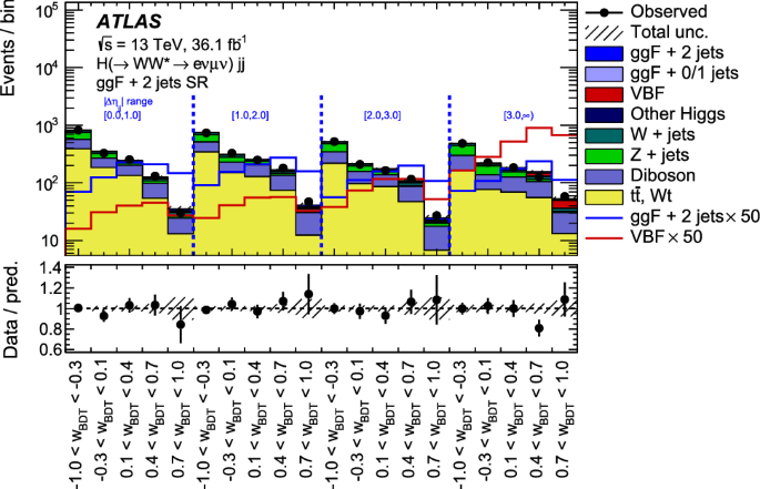

  

  Post-fit distribution of the BDT response observable presented in the four $|\Delta \eta _{jj}|$ categories of the $\mathrm {ggF}$ + 2 jets signal region, with signal and background yields fixed from the fit for $\mu ^{\mathrm {ggF}+\mathrm {2 jets}}$. Data-to-simulation ratios are shown at the bottom of the plot. The shaded areas depict the total uncertainty. The distributions of the $\mathrm {ggF}$ + 2 jets and VBF processes are overlaid with their respective contributions multiplied by 50

  Fig. 4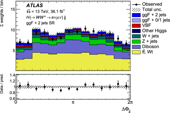

  

  The weighted $\Delta \Phi _{jj}$ post-fit distribution in the $\mathrm {ggF}$ + 2 jets signal region, with signal and background yields fixed from the fit to $\tan (\alpha )$ using shape and rate information. Data-to-simulation ratios are shown at the bottom of the plot. The shaded areas depict the total uncertainty

  Table 6 Post-fit event yields in the signal and control regions obtained from the study of the signal strength parameter $\mu ^\mathrm {ggF + 2 jets}$. The quoted uncertainties include those from theoretical and experimental systematic sources and those due to sample statistics. The fit constrains the total expected yield to the observed yield. The diboson background is split into WW and non-WW contributions

  Using rate information in addition to the shape in the fit increases the sensitivity to distinguish between the various benchmark points.⁶ However, the rate can be affected by multiple BSM effects, while the shape isolates CP-dependent variations.

• A simultaneous fit of the coupling-strength scale factors $\kappa ^{}_{gg}\cos (\alpha )$ and $\kappa ^{}_{gg}\sin (\alpha )$ is performed. This study exploits both shape and rate information.

Fig. 5

Expected and observed likelihood curves for scans a over $\tan (\alpha )$ where only the shape is taken into account in the fit, and b over $\tan (\alpha )$ when both shape and normalisation are used

The inclusive $\mathrm {ggF}$ production process is split into two components, one describing contributions from $\mathrm {ggF}$ + 0/1 jets and the other $\mathrm {ggF}$ + 2 or more jets, where only the latter one is sensitive to the CP nature of the effective Higgs–gluon coupling. The treatment of these two components varies between the different fit types. For scans over $\tan (\alpha )$ where only the shape is used, the normalisation of the $\mathrm {ggF}$ + 2 jets component floats freely in the fit, while the normalisation of the $\mathrm {ggF}$ + 0/1 jets component may vary taking into account its uncertainties. The normalisations of both components are scaled consistently to the model predictions when rates are used in the fit.

The post-fit distribution of the inputs to the signal strength parameter $\mu ^\mathrm {ggF + 2 jets}$ determination is depicted in Fig. 3. The normalised $\Delta \Phi _{jj}$ distribution in the various event categories of the $\mathrm {ggF}$ + 2 jets signal region is depicted in Fig. 4. Events are weighted by $\ln (1+N_\mathrm {S}/N_\mathrm {B})$, where $N_\mathrm {S}$ ($N_\mathrm {B}$) is the post-fit signal (background) event yield for each event category. This distribution is presented for the minimum of the NLL curve from the fit configuration that exploits both shape and rate information. The post-fit event yields in the signal region and the various control regions are presented in Table 6.

Table 7 Breakdown of the main contributions to the total uncertainty in $\tan (\alpha )$ based on the fit that exploits both shape and rate information. Individual sources of systematic uncertainty are grouped into either the theoretical or the experimental uncertainty. The sum in quadrature of the individual components differs from the total uncertainty due to correlations between the components

The signal strength parameter of the $\mathrm {ggF}$ + 2 jets process is found to be $\mu ^{\mathrm {ggF + 2 jets}}= 0.5 \pm 0.4 (\mathrm {stat.}) ^{+0.7}_{-0.6} (\mathrm {syst.})$, which is consistent with the SM prediction. The observed and expected likelihood curves corresponding to scans over $\tan (\alpha )$ are presented in Fig. 5. The values of the NLL are evaluated in steps of $\Delta \left( \tan (\alpha )\right) = 0.2$, and the minima of all fits are consistent with zero, i.e. the SM hypothesis. If only the shape information is used, the data are not sensitive enough to provide $68\%$ confidence level (CL) intervals on $\tan (\alpha )$. The ML fit configuration that uses both shape and rate information provides a best-fit value of $\tan (\alpha ) = 0.0 \pm 0.4 (\mathrm {stat.}) \pm 0.3 (\mathrm {syst.})$ for both the fits to data and to Asimov data. The observed sensitivity is slightly worse than the expected sensitivity due to a lower than expected signal yield (consistent with a signal strength value below unity). Hence, the fit to this dataset does not provide a $95\%$ CL interval. The relative impact of the main uncertainties on $\tan (\alpha )$ is presented in Table 7.

The $68\%$ and $95\%$ CL two-dimensional likelihood contours of the simultaneous scan over the CP-even and CP-odd coupling strength parameters $\kappa ^{}_{gg}\cos (\alpha )$ and $\kappa ^{}_{gg}\sin (\alpha )$ are presented in Fig. 6. Two minima are found, as the signal rate depends on the square of both couplings. The best-fit values observed in the data are consistent with the SM predictions within the $68\%$ CL, while $|\kappa ^{}_{gg} \cos (\alpha )|$ values above 1.6 and $|\kappa ^{}_{gg}\sin (\alpha )|$ values above 1.1 are excluded at $95\%$ CL.⁷

Fig. 6

$68\%$ and $95\%$ CL two-dimensional likelihood contours of the CP-even and CP-odd coupling parameters $\kappa ^{}_{gg}\cos (\alpha )$ and $\kappa ^{}_{gg}\sin (\alpha )$. The minima are represented by black stars, while the SM point is shown as a red star

Fig. 7

The weighted $\Delta \Phi _{jj}$ distribution in the VBF signal region, with signal and background yields fixed from the fit for $\varepsilon _{VV}$ using shape and rate information. Data-to-simulation ratios are shown at the bottom of the plot. The shaded areas depict the total uncertainty

8.2 VBF category

To constrain the polarisation-dependent coupling-strength scale factors in the VBF production process, the signal region and background control regions defined in Tables 3 and 4 are used as inputs to the ML fit. In the signal region, the distribution of the signed $\Delta \Phi _{jj}$ observable is used in the four categories defined by the BDT-score intervals $[-1,0.26,0.61,0.86,1]$, following Ref. [20]. The first (last) interval corresponds to the enhanced background (signal) phase-space region. No shape information is used in the control regions.

Several types of fits are performed in the VBF event category with both $(a_{\mathrm {L}}, a_{\mathrm {T}})$ and $(\kappa _{VV}, \varepsilon _{VV})$ parameterisations:

• One-dimensional fits are performed

  • using only the dependence of the input distribution’s shape on the selected parameter of interest, with the other parameter fixed to its SM value;

  • exploiting both shape and rate information, fixing one parameter to its SM value.

  The parameters $a_{\mathrm {L}}$ and $\kappa _{VV}$ dominantly affect the total event yields because the longitudinal polarisation vectors of the massive gauge bosons are proportional to the energy and can give large enhancements to the total cross section. These parameters are only weakly constrained by the shape of the $\Delta \Phi _{jj}$ distribution. The parameters $a_{\mathrm {T}}$ and $\varepsilon _{VV}$, on the other hand, affect the shape of the $\Delta \Phi _{jj}$ distribution and can be constrained from both types of fits. The kinematic distributions of the two tagging jets are related to the intrinsic structure of the Higgs boson production vertex and carry information about the polarisation of the fusing gauge bosons.

• Fits to one parameter are performed with the other being profiled.⁸ In these fits, both parameters may vary independently in order to probe them in a model-independent way.

Table 8 Post-fit event yields in the signal and control regions obtained from a scan over $\varepsilon _{VV}$ exploiting both shape and rate information. The quoted uncertainties include those from theoretical and experimental systematic sources and those due to sample statistics. The fit constrains the total expected yields to the observed yields. The diboson background is split into WW and non-WW contributions

Fig. 8

Likelihood scans over the transversely (a, b) and longitudinally (c) polarised couplings. Fits using shape-only (a) and shape+rate (b, c) information are shown. All relevant experimental and modelling systematic uncertainties are considered in the fits

Table 9 Best-fit values and their uncertainties as obtained from the shape-only and shape-plus-rate likelihood fits to the Asimov dataset and to ATLAS data. Results of both the shape-only and shape+rate fits for $a_{\mathrm {L}}$ and $a_{\mathrm {T}}$ are shown. Results of fits to one parameter with the other one fixed or profiled are presented

Table 10 Best-fit values and their uncertainties as obtained from the shape-only and shape-plus-rate likelihood fits to the Asimov dataset and to ATLAS data. Results of both shape-only and shape+rate fits for $\varepsilon _{VV}$ and $\kappa _{VV}$ are shown. Results of fits to one parameter with the other one fixed or profiled are presented

Table 11 The contributions of the leading individual systematic uncertainties together with the data statistical uncertainties, in the one-dimensional fit for the pseudo-observables $\kappa _{VV}$ (a) and $\varepsilon _{VV}$ (b) for electroweak-boson polarisation in the $\mathrm {VBF}$ $H\rightarrow WW$ channel. Both the shape and rate information is exploited in the fit. The theoretical and experimental uncertainties are subdivided further into categories

Fig. 9

Likelihood scans over a $\kappa _{VV}$ and b $\varepsilon _{VV}$, with the other parameter profiled. The fits are performed using both shape and rate information. All relevant experimental and theoretical systematic uncertainties are considered in the fits

Figure 7 depicts the weighted $\Delta \Phi _{jj}$ distribution in all categories of the VBF signal region. Events are weighted by $\ln (1+N_\mathrm {S}/N_\mathrm {B})$ in their corresponding event category. The post-fit event yields in the signal and the control regions are presented in Table 8. The results of the likelihood scans are given in Fig. 8. The scan over $a_{\mathrm {L}}$ ($a_{\mathrm {T}}$) is shown in the upper (lower) panel. Both scans have been performed in two configurations: the LLH curves shown in Fig. 8b and c are the results of the fit in which both the shape and normalisation of the signal are taken into account, while the LLH curves in Fig. 8a are obtained using only the shape information. The largest sensitivity to $a_\mathrm {L}$ stems from the rate information. The asymmetry of the curves results from the asymmetric behaviour of the cross section with respect to the changes in the parameter values (see Ref. [27]). The expected sensitivity to $a_\mathrm {T}$ comes predominantly from the shape information, as the likelihood ratio increases only slightly when adding the normalisation information. The resulting best-fit values and their uncertainties computed at $68\%$ CL are presented in Table 9. All measurements are consistent with the SM expectations. The dominant sources of uncertainty are related to the limited data yields and to the uncertainties in modelling the top-quark and WW backgrounds.

The results of the ML scans of pseudo-observables are shown in Table 10, with the uncertainty breakdown given in Table 11. Figure 9 shows the expected and observed likelihood curves for scans over one pseudo-observable with the other one profiled. Both shape and rate information are employed.

9 Conclusion

This article presents constraints on the CP structure of gluon–gluon fusion Higgs boson production and on the polarisations of the vector bosons in the HVV coupling. The results are obtained using $H(\rightarrow WW^*\rightarrow e\nu \mu \nu ) jj$ final states in data corresponding to 36.1 fb$^{-1}$ of $\sqrt{s} = 13\;\text {TeV}$ proton–proton collisions recorded by the ATLAS detector at the LHC in 2015–2016. Total event yields as well as shapes of selected kinematical distributions in signal and control regions are exploited.

The signal strength parameter for the $\mathrm {ggF}$ + 2 jets Higgs boson production mode is found to be $\mu ^{\mathrm {ggF + 2 jets}} = 0.5 \pm 0.4 (\mathrm {stat.}) ^{+0.7}_{-0.6} (\mathrm {syst.})$. The mixing angle for CP-even and CP-odd contributions to the effective Higgs–gluon interaction is determined to be $\tan (\alpha ) = 0.0 \pm 0.4 (\mathrm {stat.}) \pm 0.3 (\mathrm {syst.})$ using both shape and rate information. These results are obtained with novel analysis techniques and complement existing studies of the CP properties of the Higgs boson performed using ttH production.

The reported results for the VBF Higgs boson production mode include constraints on coupling-strength form factors to longitudinally and transversely polarised W and Z bosons. It is the first such measurement of the Higgs couplings performed. In one-dimensional ML fits (where the other parameter was set to its SM value) shape information is sufficient to constrain the coupling to transversely polarised bosons, $a_\mathrm {T}$, while to constrain $a_\mathrm {L}$ the information about the rates significantly improves the sensitivity. Profiling the other coupling-strength scale factor results in: $a_\mathrm {L}=0.91^{+0.10}_{-0.18}$(stat.)$^{+0.09}_{-0.17}$(syst.) and $a_{\mathrm {T}}=1.2 \pm 0.4$(stat.)$^{+0.2}_{-0.3}$(syst.), while $a_{\mathrm {L}}=1.00^{+0.08}_{-0.10}$(stat.)$^{+0.08}_{-0.13}$(syst.) and $a_{\mathrm {T}}=1.0^{+0.4}_{-0.5}$(stat.)$^{+0.2}_{-0.4}$(syst.) are expected in the SM.

With an approximate mapping to pseudo-observables the following constraints are obtained in a fit where the other parameter is profiled: $\kappa _{VV}= 0.91^{+0.10}_{-0.18}$(stat.)$^{+0.09}_{-0.17}$(syst.) and $\epsilon _{VV} =0.13^{+0.28}_{-0.20}$ (stat.)$^{+0.08}_{-0.10}$(syst.), while $\kappa _{VV}=1.00^{+0.08}_{-0.10}$(stat.)$^{+0.08}_{-0.13}$(syst.) and $\epsilon _{VV}=0.00^{+0.22}_{-0.24}$ (stat.)$^{+0.11}_{-0.15}$(syst.) are expected. In this parameterisation the sensitivity to the on-shell coupling $\kappa _{VV}$ is affected by the event yields, while the off-shell coupling $\varepsilon _{VV}$ is sensitive to both shape and rate information. All measurements are consistent with the expectations for the SM Higgs boson.

References

ATLAS Collaboration, Observation of a new particle in the search for the Standard Model Higgs boson with the ATLAS detector at the LHC. Phys. Lett. B 716, 1 (2012). https://doi.org/10.1016/j.physletb.2012.08.020arXiv:1207.7214 [hep-ex]
CMS Collaboration, Observation of a new boson at a mass of 125 GeV with the CMS experiment at the LHC. Phys. Lett. B 716, 30 (2012). https://doi.org/10.1016/j.physletb.2012.08.021arXiv:1207.7235 [hep-ex]
ATLAS and CMS Collaborations, Combined Measurement of the Higgs Boson Mass in pp Collisions at \(\sqrt{s}=7\, and\,8\, TeV\) with the ATLAS and CMS Experiments. Phys. Rev. Lett. 114, 191803 (2015). https://doi.org/10.1103/PhysRevLett.114.191803arXiv:1503.07589 [hep-ex]
ATLAS Collaboration, Evidence for the spin-0 nature of the Higgs boson using ATLAS data. Phys. Lett. B 726, 120 (2013). https://doi.org/10.1016/j.physletb.2013.08.026arXiv:1307.1432 [hep-ex]
ATLAS Collaboration, Study of the spin and parity of the Higgs boson in diboson decays with the ATLAS detector. Eur. Phys. J. C 75, 476 (2015) (Erratum: Eur. Phys. J. C 76 (2016) 152). https://doi.org/10.1140/epjc/s10052-016-3934-y. arXiv:1506.05669 [hep-ex]
CMS Collaboration, Study of the mass and spin-parity of the Higgs boson candidate via its decays to Z Boson pairs. Phys. Rev. Lett. 110, 081803 (2013). https://doi.org/10.1103/PhysRevLett.110.081803. arXiv:1212.6639 [hep-ex]
ATLAS Collaboration, Test of CP invariance in vector-boson fusion production of the Higgs boson in the H \(\rightarrow {\tau \tau }\) channel in proton–proton collisions at \(\sqrt{s}=13 TeV\) with the ATLAS detector. Phys. Lett. B 805, 135426 (2020). https://doi.org/10.1016/j.physletb.2020.135426. arXiv:2002.05315 [hep-ex]
CMS Collaboration, Constraints on anomalous HVV couplings from the production of Higgs bosons decaying to \(\tau \) lepton pairs. Phys. Rev. D 100, 112002 (2019). https://doi.org/10.1103/PhysRevD.100.112002. arXiv:1903.06973 [hep-ex]
CMS Collaboration, Combined search for anomalous pseudoscalar HVV couplings in VH(H \(\rightarrow {b}{\bar{b}}\)) production and H \(\rightarrow VV\) decay. Phys. Lett. B 759, 672 (2016). https://doi.org/10.1016/j.physletb.2016.06.004. arXiv:1602.04305 [hep-ex]
ATLAS Collaboration, CP Properties of Higgs Boson Interactions with Top Quarks in the t\({\bar{t}}\)H and tH Processes Using H \(\rightarrow {\gamma \gamma }\) with the ATLAS Detector. Phys. Rev. Lett. 125, 061802 (2020). https://doi.org/10.1103/PhysRevLett.125.061802. arXiv:2004.04545 [hep-ex]
CMS Collaboration, Measurements of t\({\bar{t}}\)H Production and the CP Structure of the Yukawa Interaction between the Higgs Boson and Top Quark in the Diphoton Decay Channel. Phys. Rev. Lett. 125, 061801 (2020). https://doi.org/10.1103/PhysRevLett.125.061801. arXiv:2003.10866 [hep-ex]
CMS Collaboration, Analysis of the CP structure of the Yukawa coupling between the Higgs boson and \(\tau \) leptons in proton–proton collisions at \(\sqrt{s}=13 TeV\) (2021). arXiv:2110.04836 [hep-ex]
M. Dolan et al., Constraining CP-violating Higgs Sectors at the LHC using gluon fusion. Phys. Rev. D 90, 073008 (2014). https://doi.org/10.1103/PhysRevD.90.073008arXiv:1406.3322 [hep-ph]
ATLAS Collaboration, Measurements of Higgs boson properties in the diphoton decay channel with 36 fb\(^{-1}\) of pp collision data at \(\sqrt{s}=13 TeV\) with the ATLAS detector. Phys. Rev. D 98, 052005 (2018). https://doi.org/10.1103/PhysRevD.98.052005. arXiv:1802.04146 [hep-ex]
CMS Collaboration, Constraints on anomalous Higgs boson couplings to vector bosons and fermions in its production and decay using the four-lepton final state. Phys. Rev. D 104, 052004 (2021). https://doi.org/10.1103/PhysRevD.104.052004. arXiv:2104.12152 [hep-ex]
ATLAS Collaboration, Constraints on non-Standard Model Higgs boson interactions in an effective Lagrangian using differential cross sections measured in the H \(\rightarrow {\gamma \gamma }\) decay channel at \(\sqrt{s}=8 TeV\) with the ATLAS detector. Phys. Lett. B 753, 69 (2016). https://doi.org/10.1016/j.physletb.2015.11.071. arXiv:1508.02507 [hep-ex]
CMS Collaboration, Measurements of properties of the Higgs boson decaying to a W boson pair in pp collisions at \(\sqrt{s}=13 TeV\). Phys. Lett. B 791, 96 (2019). https://doi.org/10.1016/j.physletb.2018.12.073. arXiv:1806.05246 [hep-ex]
CMS Collaboration, Measurements of the Higgs boson width and anomalous HVV couplings from on-shell and off-shell production in the four-lepton final state. Phys. Rev. D 99, 112003 (2019). https://doi.org/10.1103/PhysRevD.99.112003. arXiv:1901.00174 [hep-ex]
ATLAS Collaboration, Search for Higgs bosons produced via vector-boson fusion and decaying into bottom quark pairs in \(\sqrt{s}=13 TeV\) pp collisions with the ATLAS detector. Phys. Rev. D 98, 052003 (2018). https://doi.org/10.1103/PhysRevD.98.052003. arXiv:1807.08639 [hep-ex]
ATLAS Collaboration, Measurements of gluon-gluon fusion and vector-boson fusion Higgs boson production cross-sections in the \(H \rightarrow {WW^{*}}\,\rightarrow ev{\mu }v\,decay\) channel in pp collisions at \(\sqrt{s}=13 TeV\)with the ATLAS detector. Phys. Lett. B 789, 508 (2019). https://doi.org/10.1016/j.physletb.2018.11.064. arXiv:1808.09054 [hep-ex]
D.B. Kaplan et al., \(SU(2)\times U(1)\) breaking by vacuum misalignment. Phys. Lett. B 136, 183 (1984). https://doi.org/10.1016/0370-2693(84)91177-8
D.B. Kaplan et al., Composite Higgs scalars. Phys. Lett. B 136, 187 (1984). https://doi.org/10.1016/0370-2693(84)91178-X
P. Artoisenet et al., A framework for Higgs characterisation. JHEP 11, 043 (2013). https://doi.org/10.1007/JHEP11(2013)043. arXiv:1306.6464 [hep-ph]
J. Alwall et al., The automated computation of tree-level and next-to-leading order differential cross sections, and their matching to parton shower simulations. JHEP 07, 079 (2014). https://doi.org/10.1007/JHEP07(2014)079arXiv:1405.0301 [hep-ph]
S. Frixione et al., Matching NLO QCD computations and parton shower simulations. JHEP 0206, 029 (2002). https://doi.org/10.1088/1126-6708/2002/06/029. arXiv:hep-ph/0204244
F. Maltoni et al., Higgs characterisation at NLO in QCD: CP properties of the top-quark Yukawa interaction. Eur. Phys. J. C 74, 3065 (2014). https://doi.org/10.1140/epjc/s10052-014-3065-2arXiv:1407.5089 [hep-ph]
J. Brehmer et al., Polarized WW scattering on the Higgs pole. Phys. Rev. D 90, 054023 (2014). https://doi.org/10.1103/PhysRevD.90.054023arXiv:1404.5951 [hep-ph]
A. Greljo et al., Electroweak Higgs production with HIGGSPO at NLO QCD. Eur. Phys. J. C 77, 838 (2017). https://doi.org/10.1140/epjc/s10052-017-5422-4arXiv:1710.04143 [hep-ph]
M. Gonzalez-Alonso et al., Pseudo-observables in Higgs decays. Eur. Phys. J. C 75, 128 (2015). https://doi.org/10.1140/epjc/s10052-015-3345-5arXiv:1412.6038 [hep-ph]
ATLAS Collaboration, Measurement of inclusive and differential cross sections in the \(H \rightarrow ZZ^{*}\rightarrow 4 \ell \) decay channel in pp collisions at \(\sqrt{s}=13 TeV\) with the ATLAS detector. JHEP 10, 132 (2017). https://doi.org/10.1007/JHEP10(2017)132. arXiv:1708.02810 [hep-ex]
ATLAS Collaboration, Higgs boson production cross-section measurements and their EFT interpretation in the 4\(\ell \) decay channel at \(\sqrt{s}=13 TeV\) with the ATLAS detector, Eur. Phys. J. C 80 (2020) 957. https://doi.org/10.1140/epjc/s10052-020-8227-9 (Erratum: Erratum: Eur. Phys. J. C 81 (2021) 398). arXiv:2004.03447 [hep-ex]
T. Sjöstrand et al., A Brief Introduction to PYTHIA 8.1. Comput. Phys. Commun. 178, 852 (2008). https://doi.org/10.1016/j.cpc.2008.01.036. arXiv:0710.3820 [hep-ph]
ATLAS Collaboration, The ATLAS Experiment at the CERN Large Hadron Collider. JINST 3, S08003 (2008). https://doi.org/10.1088/1748-0221/3/08/S08003
ATLAS Collaboration, ATLAS data quality operations and performance for 2015–2018 data-taking. JINST 15, P04003 (2020). https://doi.org/10.1088/1748-0221/15/04/P04003. arXiv:1911.04632 [physics.ins-det]
ATLAS Collaboration, Improved luminosity determination in pp collisions at \(\sqrt{s}=7 TeV\) using the ATLAS detector at the LHC. Eur. Phys. J. C 73, 2518 (2013). https://doi.org/10.1140/epjc/s10052-013-2518-3. arXiv:1302.4393 [hep-ex]
ATLAS Collaboration, ATLAS Pythia 8 tunes to 7 TeV data, tech. rep. ATL-PHYS-PUB-2014-021, CERN, 2014, https://cds.cern.ch/record/1966419
R. Ball et al., Parton distributions for the LHC run II. JHEP 04, 040 (2015). https://doi.org/10.1007/JHEP04(2015)040arXiv:1410.8849 [hep-ph]
F. Demartinetal., ‘Higgs characterisation:NLO and parton-shower effects’, 2nd Toyama International Workshop on Higgs as a Probe of New Physics (2015). arXiv:1505.07081 [hep-ph]
S. Alioli et al., A general framework for implementing NLO calculations in shower Monte Carlo programs: the POWHEG BOX. JHEP 06, 043 (2010). https://doi.org/10.1007/JHEP06(2010)043arXiv:1002.2581 [hep-ph]
G. Luisoni et al., \(HW^{\pm }/HZ\) + 0 and 1 jet at NLO with the POWHEG BOX interfaced to GoSam and their merging within MiNLO. JHEP 10, 083 (2013). https://doi.org/10.1007/JHEP10(2013)083arXiv:1306.2542 [hep-ph]
ATLAS Collaboration, Measurement of the \(Z/\gamma ^{*}\) boson transverse momentum distribution in pp collisions at \(\sqrt{s}=7 TeV\) with the ATLAS detector. JHEP 09, 145 (2014). https://doi.org/10.1007/JHEP09(2014)145. arXiv:1406.3660 [hep-ex]
Jon Butterworth et al., PDF4LHC recommendations for LHC Run II. J. Phys. G 43, 023001 (2016). https://doi.org/10.1088/0954-3899/43/2/023001arXiv:1510.03865 [hep-ph]
A. Djouadi et al., HDECAY: a program for Higgs boson decays in the Standard Model and its supersymmetric extension. Comput. Phys. Commun. 108, 56 (1998). https://doi.org/10.1016/S0010-4655(97)00123-9arXiv:hep-ph/9704448
LHC Higgs Cross Section Working Group, Handbook of LHC Higgs Cross Sections: 4. Deciphering the Nature of the Higgs Sector (2016). arXiv:1610.07922 [hep-ph]
M. Cacciari et al., Fully Differential Vector-Boson-Fusion Higgs Production at Next-to-Next-to-Leading Order, Phys. Rev. Lett. 115, 082002 (2015). https://doi.org/10.1103/PhysRevLett.115.082002 (Erratum: Phys. Rev. Lett. 120 (2018) 139901). arXiv:1506.02660 [hep-ph]
A. Denner et al., HAWK 2.0: A Monte Carlo program for Higgs production in vector-boson fusion and Higgs strahlung at hadron colliders. Comput. Phys. Commun. 195, 161 (2015). https://doi.org/10.1016/j.cpc.2015.04.021arXiv:1412.5390 [hep-ph]
J.M. Lindert et al., An NLO+PS generator for \(t{\bar{t}}\) and Wt production and decay including non-resonant and interference effects. Eur. Phys. J. C 76, 691 (2016). https://doi.org/10.1140/epjc/s10052-016-4538-2arXiv:1607.04538 [hep-ph]
M. Czakon et al., Top++: a program for the calculation of the top-pair cross-section at hadron colliders. Comput. Phys. Commun. 185, 2930 (2011). https://doi.org/10.1016/j.cpc.2014.06.021arXiv:1112.5675 [hep-ph]
P.Z. Skands et al., Tuning Monte Carlo generators: the Perugia tunes. Phys. Rev. D 82, 074018 (2010). https://doi.org/10.1103/PhysRevD.82.074018arXiv:1005.3457 [hep-ph]
H.L. Lai et al., New parton distributions for collider physics. Phys. Rev. D 82, 074024 (2010). https://doi.org/10.1103/PhysRevD.82.074024arXiv:1007.2241 [hep-ph]
S. Frixione et al., Single-top hadroproduction in association with a W boson. JHEP 07, 029 (2008). https://doi.org/10.1088/1126-6708/2008/07/029arXiv:0805.3067 [hep-ph]
T. Gleisberg et al., Event generation with SHERPA 1.1. JHEP 0902, 007 (2009). https://doi.org/10.1088/1126-6708/2009/02/007arXiv:0811.4622 [hep-ph]
E. Bothmann et al., Event generation with SHERPA 2.2, SciPost Physics 7 (2019), ISSN: 2542-4653. https://doi.org/10.21468/SciPostPhys.7.3.034
ATLAS Collaboration, Multi-Boson Simulation for 13 TeV ATLAS Analyses, tech. rep. ATL-PHYS-PUB-2017-005, CERN (2017). https://cds.cern.ch/record/2261933
S. Hoeche et al., QCD matrix elements + parton showers. The NLO case. JHEP 04, 027 (2013). https://doi.org/10.1007/JHEP04(2013)027. arXiv:1207.5030 [hep-ph]
F. Cascioli et al., Scattering amplitudes with open loops. Phys. Rev. Lett. 108, 111601 (2012). https://doi.org/10.1103/PhysRevLett.108.111601arXiv:1111.5206 [hep-ph]
ATLAS Collaboration, The ATLAS simulation infrastructure. Eur. Phys. J. C 70, 823 (2010). https://doi.org/10.1140/epjc/s10052-010-1429-9. arXiv:1005.4568 [physics.ins-det]
GEANT4 Collaboration, GEANT4-a simulation toolkit. Nucl. Instrum. Methods A 506, 250 (2003). https://doi.org/10.1016/S0168-9002(03)01368-8
ATLAS Collaboration, Performance of electron and photon triggers in ATLAS during LHC Run 2. Eur. Phys. J. C 80, 47 (2020). https://doi.org/10.1140/epjc/s10052-019-7500-2. arXiv:1909.00761 [hep-ex]
ATLAS Collaboration, Performance of the ATLAS muon triggers in Run 2. JINST 15, P09015 (2020). https://doi.org/10.1088/1748-0221/15/09/p09015. arXiv:2004.13447 [physics.ins-det]
ATLAS Collaboration, Performance of the ATLAS trigger system. Eur. Phys. J. C 77(2017), 317 (2015). https://doi.org/10.1140/epjc/s10052-017-4852-3. arXiv:1611.09661 [hep-ex]
ATLAS Collaboration, Electron reconstruction and identifcation in the ATLAS experiment using the 2015 and 2016 LHC proton-proton collision data at \(\sqrt{s}=13 TeV\). Eur. Phys. J. C 79, 639 (2019). https://doi.org/10.1140/epjc/s10052-019-7140-6. arXiv:1902.04655 [physics.ins-det]
ATLAS Collaboration, Muon reconstruction performance of the ATLAS detector in proton-proton collision data at \(\sqrt{s}=13 TeV\). Eur. Phys. J. C 292, 76 (2016). https://doi.org/10.1140/epjc/s10052-016-4120-y. arXiv:1603.05598 [hep-ex]
ATLAS Collaboration, Topological cell clustering in the ATLAS calorimeters and its performance in LHC Run 1. Eur. Phys. J. C 77, 490 (2017). https://doi.org/10.1140/epjc/s10052-017-5004-5. arXiv:1603.02934 [hep-ex]
G.S. Salam et al., The anti-k\(_{t}\) jet clustering algorithm. JHEP 0804, 063 (2008). https://doi.org/10.1088/1126-6708/2008/04/063arXiv:0802.1189 [hep-ph]
M. Cacciari et al., FastJet user manual. Eur. Phys. J. C 72, 1896 (2012). https://doi.org/10.1140/epjc/s10052-012-1896-2arXiv:1111.6097 [hep-ph]
ATLAS Collaboration, Jet energy scale measurements and their systematic uncertainties in proton-proton collisions at \(\sqrt{s}=13 TeV\) with the ATLAS detector. Phys. Rev. D 96, 072002 (2017). https://doi.org/10.1103/PhysRevD.96.072002. arXiv:1703.09665 [hep-ex]
ATLAS Collaboration, Tagging and suppression of pileup jets, tech. rep. ATLAS-CONF-2014-018, CERN (2014). https://cds.cern.ch/record/1700870
ATLAS Collaboration, Identifcation and rejection of pile-up jets at high pseudorapidity with the ATLAS detector, Eur. Phys. J. C 77 (2017) 580, https://doi.org/10.1140/epjc/s10052-017-5245-3 (Erratum: Eur. Phys. J. C 77 (2017) 712). arXiv:1705.02211 [hep-ex]
ATLAS Collaboration, Performance of b-Jet Identification in the ATLAS Experiment. JINST 11, P04008 (2016). https://doi.org/10.1088/1748-0221/11/04/P04008. arXiv:1512.01094 [hep-ex]
ATLAS Collaboration, Optimisation of the ATLAS b-tagging performance for the 2016 LHC Run,tech. rep. ATL-PHYS-PUB-2016-012, CERN (2016) https://cds.cern.ch/record/2160731
ATLAS Collaboration, \(E_{T}^{miss}\) performance in the ATLAS detector using 2015–2016 LHC pp collisions, ATLAS-CONF-2018-023 (2018) https://cds.cern.ch/record/2625233
T. Plehn et al., A Method for identifying H \(\rightarrow \tau ^{+}\tau ^{-} \rightarrow e^{\pm } \mu ^{\mp } P_{T}\)at the CERN LHC. Phys. Rev. D 61, 093005 (2000). https://doi.org/10.1103/PhysRevD.61.093005. arXiv:hep-ph/9911385
ATLAS Collaboration, Measurements of b-jet tagging effciency with the ATLAS detector using \(t{\bar{t}}\) events at \(\sqrt{s}=13 TeV\). JHEP 08, 089 (2018). https://doi.org/10.1007/JHEP08(2018)089. arXiv:1805.01845 [hep-ex]
ATLAS Collaboration, Electron and photon energy calibration with the ATLAS detector using 2015-2016 LHC proton-proton collision data. JINST 14, P03017 (2019). https://doi.org/10.1088/1748-0221/14/03/P03017. arXiv:1812.03848 [hep-ex]
ATLAS Collaboration, Luminosity determination in pp collisions at \(\sqrt{s}=13 TeV\) using the ATLAS detector at the LHC, ATLAS-CONF-2019-021 (2019). https://cds.cern.ch/record/2677054
J. Bellm et al., Herwig 7.0/Herwig++ 3.0 release note. Eur. Phys. J. C 76, 196 (2016). https://doi.org/10.1140/epjc/s10052-016-4018-8arXiv:1512.01178 [hep-ph]
M.H. Seymour et al., Constraining MPI models using \({ }_{eff}\) and recent Tevatron and LHC Underlying Event data. JHEP 10, 113 (2013). https://doi.org/10.1007/JHEP10(2013)113arXiv:1307.5015 [hep-ph]
J. Bellm et al., Herwig++ 2.7 Release Note (2013). arXiv:1310.6877 [hep-ph]
C.D. White et al., Isolating Wtproduction at the LHC. JHEP 11, 074 (2009). https://doi.org/10.1088/1126-6708/2009/11/074arXiv:0908.0631 [hep-ph]
R. Frederix et al., Merging meets matching in MC@NLO. JHEP 12, 061 (2012). https://doi.org/10.1007/JHEP12(2012)061arXiv:1209.6215 [hep-ph]
G. Cowan et al., Asymptotic formulae for likelihood-based tests of new physics, Eur. Phys. J. C 71 (2011) 1554, https://doi.org/10.1140/epjc/s10052-011-1554-0 (Erratum: Eur. Phys. J. C 73, 2501 (2013)). arXiv:1007.1727 [physics.data-an]
ATLAS Collaboration, A morphing technique for signal modelling in a multidimensional space of coupling parameters, tech. rep. ATL-PHYS-PUB-2015-047, CERN (2015). https://cds.cern.ch/record/2066980
M. Baak et al., Interpolation between multi-dimensional histograms using a new non-linear moment morphing method. Nucl. Instrum. Methods A 771, 39 (2015). https://doi.org/10.1016/j.nima.2014.10.033. arXiv:1410.7388 [physics.data-an]
ATLAS Collaboration, Combined measurements of Higgs boson production and decay using up to 80 fb\(^{-1}\) of proton–proton collision data at \(\sqrt{s}=13 TeV\) collected with the ATLAS experiment, Phys. Rev. D 101, 012002 (2020). https://doi.org/10.1103/PhysRevD.101.012002
ATLAS Collaboration, ATLAS Computing Acknowledgements, ATL-SOFT-PUB-2021-003. https://cds.cern.ch/record/2776662
Acknowledgements
We thank CERN for the very successful operation of the LHC, as well as the support staff from our institutions without whom ATLAS could not be operated efficiently. We acknowledge the support of ANPCyT, Argentina; YerPhI, Armenia; ARC, Australia; BMWFW and FWF, Austria; ANAS, Azerbaijan; SSTC, Belarus; CNPq and FAPESP, Brazil; NSERC, NRC and CFI, Canada; CERN; ANID, Chile; CAS, MOST and NSFC, China; Minciencias, Colombia; MEYS CR, Czech Republic; DNRF and DNSRC, Denmark; IN2P3-CNRS and CEA-DRF/IRFU, France; SRNSFG, Georgia; BMBF, HGF and MPG, Germany; GSRI, Greece; RGC and Hong Kong SAR, China; ISF and Benoziyo Center, Israel; INFN, Italy; MEXT and JSPS, Japan; CNRST, Morocco; NWO, Netherlands; RCN, Norway; MEiN, Poland; FCT, Portugal; MNE/IFA, Romania; JINR; MES of Russia and NRC KI, Russian Federation; MESTD, Serbia; MSSR, Slovakia; ARRS and MIZŠ, Slovenia; DSI/NRF, South Africa; MICINN, Spain; SRC and Wallenberg Foundation, Sweden; SERI, SNSF and Cantons of Bern and Geneva, Switzerland; MOST, Taiwan; TAEK, Turkey; STFC, United Kingdom; DOE and NSF, USA. In addition, individual groups and members have received support from BCKDF, CANARIE, Compute Canada and CRC, Canada; COST, ERC, ERDF, Horizon 2020 and Marie Skłodowska-Curie Actions, European Union; Investissements d’Avenir Labex, Investissements d’Avenir Idex and ANR, France; DFG and AvH Foundation, Germany; Herakleitos, Thales and Aristeia programmes co-financed by EU-ESF and the Greek NSRF, Greece; BSF-NSF and GIF, Israel; Norwegian 2014-2021, Norway; NCN and NAWA, Poland; La Caixa Banking Foundation, CERCA Programme Generalitat de Catalunya and PROMETEO and GenT Programmes Generalitat Valenciana, Spain; Göran Gustafssons Stiftelse, Sweden; The Royal Society and Leverhulme Trust, UK. The crucial computing support from all WLCG partners is acknowledged gratefully, in particular from CERN, the ATLAS Tier-1 facilities at TRIUMF (Canada), NDGF (Denmark, Norway, Sweden), CC-IN2P3 (France), KIT/GridKA (Germany), INFN-CNAF (Italy), NL-T1 (Netherlands), PIC (Spain), ASGC (Taiwan), RAL (UK) and BNL (USA), the Tier-2 facilities worldwide and large non-WLCG resource providers. Major contributors of computing resources are listed in Ref. [86].
Author information
Authors and Affiliations
Consortia
Rights and permissions
Open Access This article is licensed under a Creative Commons Attribution 4.0 International License, which permits use, sharing, adaptation, distribution and reproduction in any medium or format, as long as you give appropriate credit to the original author(s) and the source, provide a link to the Creative Commons licence, and indicate if changes were made. The images or other third party material in this article are included in the article’s Creative Commons licence, unless indicated otherwise in a credit line to the material. If material is not included in the article’s Creative Commons licence and your intended use is not permitted by statutory regulation or exceeds the permitted use, you will need to obtain permission directly from the copyright holder. To view a copy of this licence, visit http://creativecommons.org/licenses/by/4.0/.
Funded by SCOAP3. SCOAP3 supports the goals of the International Year of Basic Sciences for Sustainable Development.
About this article
Cite this article
Aad, G., Abbott, B., Abbott, D.C. et al. Constraints on Higgs boson properties using \(WW^{*}(\rightarrow e\nu \mu \nu )jj\) production in \(36.1\,\mathrm{fb}^{-1}\) of \(\sqrt{s}=13\) TeV pp collisions with the ATLAS detector. Eur. Phys. J. C 82, 622 (2022). https://doi.org/10.1140/epjc/s10052-022-10366-1
Received:
Accepted:
Published:
DOI: https://doi.org/10.1140/epjc/s10052-022-10366-1