
Abstract
We present the new version of OpenLoops, an automated generator of tree and one-loop scattering amplitudes based on the open-loop recursion. One main novelty of OpenLoops 2 is the extension of the original algorithm from NLO QCD to the full Standard Model, including electroweak (EW) corrections from gauge, Higgs and Yukawa interactions. In this context, among several new features, we discuss the systematic bookkeeping of QCD–EW interferences, a flexible implementation of the complex-mass scheme for processes with on-shell and off-shell unstable particles, a special treatment of on-shell and off-shell external photons, and efficient scale variations. The other main novelty is the implementation of the recently proposed on-the-fly reduction algorithm, which supersedes the usage of external reduction libraries for the calculation of tree–loop interferences. This new algorithm is equipped with an automated system that avoids Gram-determinant instabilities through analytic methods in combination with a new hybrid-precision approach based on a highly targeted usage of quadruple precision with minimal CPU overhead. The resulting significant speed and stability improvements are especially relevant for challenging NLO multi-leg calculations and for NNLO applications.
1 Introduction
Scattering amplitudes at one loop are a mandatory ingredient for any precision calculation at high-energy colliders. At next-to-leading order (NLO), the calculation of hard cross sections requires one-loop matrix elements with hard kinematics, while next-to-next-to leading order (NNLO) predictions require one-loop amplitudes with one additional unresolved particle. Nowadays, thanks to a variety of modern techniques [1,2,3,4,5,6,7,8,9], one-loop calculations can be carried out with a number of automated and widely applicable programs [10,11,12,13,14,15,16,17,18,19,20] that have strongly boosted the field of precision phenomenology. Most notably, such tools have extended the reach of NLO calculations to highly non-trivial multi-particle processes [21,22,23,24,25] and have opened the door to the automation of multi-purpose Monte Carlo generators at NLO [26,27,28,29,30,31,32].
In this paper we present the new version of OpenLoops,Footnote 1 an automated tool for the calculation of tree and one-loop scattering amplitudes within the Standard Model (SM). The OpenLoops algorithm is based on a numerical recursionFootnote 2 that generates loop amplitudes in terms of cut-open loop diagrams [9, 33]. Such objects, called open loops, are characterised by a tree topology but depend on the loop momentum.
In the original version of the algorithm [9], implemented in OpenLoops 1 [16], loop amplitudes are built in two phases. In the first phase, Feynman diagrams are constructed in terms of tensor integrals using the open-loop recursion, while in the second phase, loop amplitudes are reduced to scalar integrals using external libraries such as Collier [19] or CutTools [10]. The main strengths of this approach are the high speed of the open-loop recursion and the possibility of curing numerical instabilities through the tensor-reduction techniques [4, 34] implemented in Collier [19].
In the original open-loop algorithm [9], the rank of open loops increases at each step of the recursion. As a consequence, the CPU time required for their processing, the memory footprint, and also numerical instabilities, tend to grow rather fast with the number of scattering particles. For these reasons, in OpenLoops 2 the construction of loop amplitudes and their reduction have been unified in a single recursive algorithm [33] that makes it possible to avoid high-rank objects at all stages of the amplitude calculations. This is achieved by interleaving single steps of the construction of open loops with reduction operations at the integrand level [2]. The implementation of this method, called on-the-fly reduction, is one of the main novelties of OpenLoops 2. So far it is restricted to tree–loop interferences at NLO, while squared loop amplitudes are still processed in the same way as in OpenLoops 1.
The on-the-fly reduction algorithm in OpenLoops 2 is equipped with an automated system that avoids numerical instabilities in a highly efficient way. This stability system makes use of analytic techniques that have been introduced in [33] and have meanwhile been extended in various directions, and supplemented by a novel hybrid-precision system. The latter monitors the level of stability by exploiting information on the analytic structure of the reduction identities, and residual instabilities are stabilised on-the-fly through quadruple precision (qp). This system is implemented at the level of individual operations. In this way, the usage of qp is restricted to a minimal part of the calculations, which results in a huge speed-up as compared to complete qp re-evaluations. Thanks to these features, the on-the-fly reduction method makes it possible to achieve an unprecedented level of numerical stability, both for multi-leg NLO calculations with hard kinematics and for NNLO applications with unresolved partons.
The structure of the open-loop recursion [9, 33] is model independent, and the explicit form of its kernels depends only on the Lagrangian of the model at hand. The original implementation [16] was applicable to any SM process at NLO QCD, and the other major novelty of OpenLoops 2 is the extension of NLO automation to the full SM [35, 36], including any correction effect of \(\mathcal {O}(\alpha _{\mathrm {s}})\) and \(\mathcal {O}(\alpha )\).Footnote 3 In this respect, in this paper we present a detailed discussion of the interplay of QCD and EW effects in scattering amplitudes with more than one quark chain, which are relevant for LHC processes with two or more light jets. In that case, Born amplitudes consist of towers of terms of order \(\alpha _{\mathrm {s}}^p\alpha ^q\) with fixed total power \(p+q\) but variable powers in the QCD and EW couplings. In such cases, as is well known, QCD and EW interactions mix through interference effects and, in general, NLO terms of fixed order \(\alpha _{\mathrm {s}}^P\alpha ^Q\) involve correction effects of QCD and EW kind. However, as we will point out, each NLO term of order \(\alpha _{\mathrm {s}}^P\alpha ^Q\) is always dominated either by QCD corrections to Born terms of order \(\alpha _{\mathrm {s}}^{P-1}\alpha ^Q\)or by EW corrections to Born terms of order \(\alpha _{\mathrm {s}}^{P}\alpha ^{Q-1}\).
In this paper the renormalisation of the SM and its implementation in OpenLoops are discussed in detail. In the QCD sector, quark masses and Yukawa couplings can be renormalised in the on-shell and \(\overline{\text {MS}}\) schemes, and the \(\alpha _{\mathrm {s}}\) counterterm can be flexibly adapted to any flavour-number scheme. The renormalisation of masses and couplings at \(\mathcal {O}(\alpha )\) is based on the on-shell scheme [37] and its extension to complex masses [38] for off-shell unstable particles. More precisely, in OpenLoops 2 these two approaches are unified in a generic scheme that can address processes with combinations of on-shell and off-shell unstable particles, such as for \(pp\rightarrow t {\bar{t}} \ell ^+ \ell ^-\), where Z-bosons occur as internal resonances, while top quarks are on-shell external states. Besides UV counterterms, OpenLoops 2 implements also Catani–Seymour’s \({{\mathbf {I}}}\)-operator for the subtraction of infrared (IR) singularities at \(\mathcal {O}(\alpha _{\mathrm {s}})\) [39, 40] and \(\mathcal {O}(\alpha )\) [36, 41,42,43,44].
For the definition of EW couplings, three different schemes based on the the input parameters \(\alpha (0)\), \(\alpha (M_Z^2)\) and \(G_\mu \) are supported. Moreover, OpenLoops 2 implements an automated system for the optimal choice of the coupling of on-shell and off-shell external photons. Concerning the choice of \(\alpha _{\mathrm {s}}\) and the renormalisation scale \(\mu _\mathrm{R}\), a new automated scale-variation mechanism makes it possible to re-evaluate scattering amplitudes for multiple values of \(\alpha _{\mathrm {s}}\) and \(\mu _\mathrm{R}\) with minimal CPU cost.
The OpenLoops 2 program can be combined with any other code by means of its native Fortran and C/ interfaces, which allow one to exploit its functionalities in a flexible way. Besides the choice of processes and parameters, the interfaces support the calculation of LO, NLO, and loop-induced matrix elements and building blocks thereof, as well as various colour and spin correlators relevant for the subtraction of IR singularities at NLO and NNLO. Additional interface functions give access to the SU(3) colour basis and the colour flow of tree amplitudes. Besides its native interfaces, OpenLoops offers also a standard interface in the BLHA format [45, 46].
The OpenLoops program can be used as a plug-in by the Monte Carlo programs Sherpa [26, 47], Powheg-Box [27],  [32], Geneva [48], and Whizard [49], which possess built-in interfaces that control all relevant OpenLoops functionalities in a largely automated way, requiring only little user intervention. Moreover, OpenLoops is used as a building block of Matrix [50] for the calculation of NNLO QCD observables. In this context, the automation of EW corrections in OpenLoops 2 opens the door to ubiquitous NLO QCD+NLO EW simulations in Sherpa [51, 52] and NNLO QCD+NLO EW calculations in Matrix [53].
The OpenLoops 2 code is publicly available on the Hepforge webpage
https://openloops.hepforge.org
and via the Git repository
https://gitlab.com/openloops/OpenLoops.
It consists of a process-independent base code and a process library that covers several hundred partonic processes, including essentially all relevant processes at the LHC. The desired processes can be easily accessed through an automated download mechanism. The set of available processes is continuously extended, and possible missing processes can be promptly generated by the authors upon request.
The paper is organised as follows. Section 2 presents the structure of the original open-loop recursion and the new on-the-fly reduction algorithm. Numerical instabilities and the new hybrid-precision system are discussed in detail. Section 3 deals with general aspects of NLO calculations and their automation in OpenLoops. This includes the bookkeeping of towers of terms of variable order \(\alpha _{\mathrm {s}}^p\alpha ^q\), the treatment of input parameters, optimal couplings for external photons, the renormalisation of the SM at \(\mathcal {O}(\alpha _{\mathrm {s}})\) and \(\mathcal {O}(\alpha )\), the on-shell and complex-mass schemes, and the \({{\mathbf {I}}}\)-operator. Section 4 provides instructions on how to use the program, starting from installation and process selection, and including the various interfaces for the calculation of matrix elements, colour/spin correlators, and tree amplitudes in colour space. Technical benchmarks concerning the speed and numerical stability of OpenLoops 2 are presented in Sect. 5. A detailed description of the syntax and usage of the OpenLoops interfaces can be found in the appendices.
While the paper as a whole serves as a detailed documentation of the algorithms implemented in OpenLoops 2, Sect. 4 together with Appendix A can be used alone as a manual.
2 The OpenLoops algorithm
The calculation of loop amplitudes in OpenLoops proceeds through the recursive construction of open loops and their reduction to master integrals. In this section we outline two variants of this procedure: the original open-loop method [9], which was used throughout in OpenLoops 1 and is still used for loop-induced processes in OpenLoops 2, and the new on-the-fly reduction method [33] used for tree–loop interferences in OpenLoops 2.
2.1 Scattering amplitudes and probability densities
The main task carried out by OpenLoops is the computation of the colour and helicity-summed scattering probability densities
which consist of the various interference terms that involve the Born amplitude \(\mathcal {M}_0\) and the one-loop amplitude \(\mathcal {M}_1\) for a certain process selected by the user. The usual summations and averaging over external helicitiesFootnote 4 and colours, as well as symmetry factors for identical particles, are included throughout and implicitly understood in the bra–ket notation in (2.1)–(2.3). The relevant average factors are encoded in
where \(\mathcal {S}_{\mathrm {in}}\) denotes the set of initial-state particles, while \(N_{\mathrm {hel},i}\) and \(N_{\mathrm {col},i}\) are the number of helicity and colour states of particle i. The symmetry factors depend on the number \(n_p\) of identical final-state particles. They are applied to all types of final-state particles, \(p\in {\mathcal {P}}_{\mathrm {out}}\), treating particles and anti-particles as different types.
For standard processes with \(\mathcal {M}_{0}\ne 0\), leading-order (LO) cross sections involve only squared tree contributions \(\mathcal {W}_{00}\), while at next-to-leading order (NLO) virtual one-loop contributions \(\mathcal {W}_{01}\) and real-emission contributions of type \(\mathcal {W}_{00}\) with one additional parton are needed. The squared one-loop probability density \(\mathcal {W}_{11}\) is the main LO building block for loop-induced processes, i.e. processes with \(\mathcal {M}_{0}=0\). For the calculation of such processes at NLO also \(\mathcal {W}_{11}\)-type densities with one additional parton are needed. Otherwise \(\mathcal {W}_{11}\) is relevant as ingredient of next-to-next-to-leading order (NNLO) calculations.
In OpenLoops, L-loop matrix elements \(\mathcal {M}_L\) are computed in terms of Feynman diagrams, whose structures are generated with Feynarts [54]. The Feynman diagrams are expressed as helicity amplitudes,
for \(L=0,1\). Here \(\varOmega _{L}\) is the set of all L-loop Feynman diagrams, \(h\) describes a specific helicity configuration of the external particles, and each diagram \(\mathcal {I}\) is factorised into a colour factor \({\mathcal {C}}(\mathcal {I})\) and a colour-stripped diagram amplitudeFootnote 5 \(\mathcal {A}_L(\mathcal {I},h)\). The colour structures \({\mathcal {C}}(\mathcal {I})\) are algebraically reduced to a standard colour basis \(\{{\mathcal {C}}_i\}\) (see Sect. 4.5),
where scattering amplitudes take the form
and colour-summed interferences in (2.1)–(2.3) are built by means of the colour-interference matrix
In the following we focus on the construction of the colour-stripped amplitudes \(\mathcal {A}_L(\mathcal {I},h)\).
2.2 Tree amplitudes
At tree level, each colour-stripped Feynman diagram is built by contracting two subtrees that are connected through a certain cut propagator,Footnote 6

Here \(k_{a}=-k_{b}\) and \(\sigma _a,\sigma _b\) are the momenta and spinor/ Lorentz indices of the subtrees, while \(h_a,h_b\) denote the helicity configurations of the external particles connected to the respective subtrees.Footnote 7 The tilde in \({\widetilde{w}}_b\) marks the absence of the cut propagator, which is included in \(w_a\). All relevant subtrees are generated through a numerical recursion that starts from the external wave functions and connects an increasing number of external particles through operations of the form

The tensor \(X_{\sigma _b\sigma _c}^{\sigma _a}\) corresponds to the triple vertex that connects \(w_a, w_b, w_c\), combined with the numerator of the propagator attached to \(w_a\). For quartic vertices an analogous relation is used. Each step needs to be carried out for all independent helicity configurations \(h_{b}, h_{c}\). The resulting tree recursion is implemented in an efficient way by caching the amplitudes of subtrees that contribute to multiple Feynman diagrams.
2.3 One-loop amplitudes
Renormalised one-loop amplitudes are split into three building blocks,
where \(\mathcal {M}_{1,\text {CT}}\) denotes UV counter-terms, while bare one-loop amplitudes are decomposed into a contribution that is computed with four-dimensional loop numerator (\(\mathcal {M}_{1,4\mathrm {D}}\)) plus a so-called \(R_2\) rational term stemming form the \((D-4)\)-dimensional part of loop numerators (\(\mathcal {M}_{1,R_2}\)). The latter is reconstructed via \(R_2\) counter-terms [56,57,58,59,60,61,62,63], and \(\mathcal {M}_{1,R_2}+\mathcal {M}_{1,\text {CT}}\) are generated in a similar way as tree amplitudes.
The remaining part, \(\mathcal {M}_{1,4\mathrm {D}}\), is constructed in terms of colour-stripped loop diagrams,

with four-dimensional numerators \({\mathcal {N}}({\mathcal {I}}_{N},q,h)\) and denominators \(\bar{D}_{i}(\bar{q})=(\bar{q}+ p_{i})^2-m_{i}^2\), where the bar is used for quantities in D dimensions, and the \((D-4)\)-dimensional part of the loop momentum is denoted \(\tilde{q}=\bar{q}-q\). The trace represents the contraction of spinor/Lorentz indices along the loop, and the index \(\mathcal {I}_N\) stands for the N-point topology at hand.
The numerator is computed by cut-opening the loop at a certain propagator, which results into a tree-like structure consisting of a product of loop segments,

where \(\beta _{0},\beta _{N}\) are the spinor/Lorentz indices of the cut propagator. Loop segments that are connected to the loop via triple vertices have the form

where an external subtree \(w_i\) is connected to a loop vertex and to the adjacent loop propagator. The latter correspond to a rank-one polynomial in the loop momentum with coefficients Y and Z. A similar relation is used for quartic vertices.
The loop numerator is constructed by attaching the various segments to each other through recursive dressing steps,
for \(k=1,\dots , N\), starting from the initial condition  . The labels \(h_k\) and \(\hat{h}_k\) correspond, respectively, to the helicity configuration of the external legs entering the \(k^{\mathrm {th}}\) segments and the first k segments. The partially dressed numerator (2.15) is called an open loop. Schematically it can be represented as

where blue and grey blobs correspond, respectively, to those loop segments that are already dressed and remain to be dressed. Each open loop is a polynomial in q,
and all dressing steps are implemented at the level of the open-loop tensor coefficients \(\mathcal {N}^{(k)}_{\mu _1\dots \mu _r}\).
2.4 Reduction to master integrals

Evolution of the tensor rank and the number of open-loop tensor coefficients (right vertical axis) as a function of the number k of dressed segments during the open-loop recursion. The red diagonal lines illustrate the dressing steps, and the blue vertical lines the reduction steps
In OpenLoops the reduction of loop amplitudes to master integrals is carried out with two different methods. Squared loop amplitudes and tree-loop interferences in the Higgs Effective Field Theory (HEFT)Footnote 8 are handled along the lines of the original open-loop approach [9], where the reduction is performed a posteriori of the dressing recursion. Since every dressing step can increase the tensor rank by one (see Fig. 1 a), this generates intermediate objects of high tensor rank, i.e. high complexity, with a negative impact on CPU speed. In contrast, all other tree–loop interferences are computed with the on-the-fly reduction approach [33], where dressing steps are interleaved with integrand reduction steps in such a way that the tensor rank, and thus the complexity, remain low at all stages of the calculation (see Fig. 1b).
2.4.1 A posteriori reduction
The a posteriori reduction to scalar integrals is done by means of external tools. By default, the reduction is performed at the level of tensor integrals,
using the Collier library [19], which implements the Denner–Dittmaier reduction techniques [4, 34] as well as the scalar integrals of [64]. Alternatively, the reduction can be performed at the integrand level using CutTools [10], which implements the OPP reduction method [5], in combination with the OneLOop library [65] for scalar integrals.
2.4.2 On-the-fly reduction
In the on-the-fly approach, the dressing of open loops is interleaved with reduction steps. The latter are applied in such a way that the tensor rank never exceeds two.
For objects with more than three loop propagators, \(D_0,D_1,D_2,D_3,\ldots \), the tensor rank is reduced using an integrand-reduction identity [2] of the form
with
where the coefficients \(A^{\mu \nu }_{i}\) and \(B^{\mu \nu }_{i,\lambda }\) depend on the internal masses and external momenta. The four-dimensional \(D_i\) terms on the rhs of (2.20) are cancelled against the D-dimensional loop denominators. This gives rise to \(\tilde{q}^2\) dependent terms, \(D_i/\bar{D}_{j}=1-\tilde{q}^2/\bar{D}_{j}\), which are consistently taken into account and result into rational contributions of kind \(R_1\) [2, 33]. Note that the reduction (2.20) and the pinching of propagators can be carried out as soon as rank two is reached, irrespective of which loop segments are still undressed. Every reduction step generates four new pinched sub-topologies, and the proliferation of pinched objects is avoided by means of the merging approach described in Sect. 2.5.
Rank-two open loops with only three loop denominators can be reduced on-the-fly in a similar way as open loops with more than three propagators [33]. The remaining reducible integrals have the following number of propagators N and tensor rank R: \(N\ge 5\) and \(R=1,0\); \(N=4,3\) and \(R=1\); \(N=2\) and \(R=2,1\). For their reduction to master integrals we use a combination of integral reduction and OPP reduction identities [33]. Master integrals are evaluated with Collier [19], which is the default in double precision, or OneLOop [65], which is the default in quadruple precision.
2.5 Tree–loop interference
In the following we outline the calculation of tree–loop interferences (2.2) according to the original open-loop algorithm and with the on-the-fly approach [33]. The latter is used by default in OpenLoops 2. In both cases, the colour treatment is based on the factorisation of colour structures at the level of individual loop diagrams, \(\mathcal {M}_{1}(\mathcal {I},h) = {\mathcal {C}}(\mathcal {I})\,\mathcal {A}_1(\mathcal {I},h)\). This makes it possible to cast the interference of loop diagrams with the Born amplitude into the form
where \(\mathcal {A}_1(\mathcal {I},h)\) is the colour-stripped loop amplitude, and the colour information is entirely absorbed into the colour-summed interference factor
where \(a_j(\mathcal {I})\), \(\mathcal {A}_0^{(i)}(h)\), and \(\mathcal {K}_{ij}\) are defined in (2.6)–(2.8). In this way, as detailed below, the full tree–loop interference can be constructed in terms of colour-stripped or colour-summed objects.

Example of parent-child relation between open loops. The parent N-point diagram \(\mathcal {I}_{N}\) and the child \((N-1)\)-point diagram \({\tilde{\mathcal {I}}}_{N-1}\) share the first k segments (blue blobs). Thus \(\mathcal {N}_k({\mathcal {I}}_{N},q)\) and \(\mathcal {N}_k(\tilde{{\mathcal {I}}}_{N-1},q)\) are identical and need to be constructed only once
2.5.1 Parent-child algorithm
In the original open-loop approach, tree–loop interference contributions of type (2.21) are constructed as follows.
- (i)
The numerator of a colour-stripped N-point loop diagram (2.12) is constructed as outlined in Sect. 2.3, i.e. starting from
 and applying N dressing steps of type (2.15).
 - (ii)
In general, open loops with higher number N of loop propagators do not need to be built from scratch, but can be constructed starting form pre-computed open loops with lower N exploiting parent–child relations [9] as illustrated in Fig. 2. The efficiency of the parent–child approach is maximised by means of cutting rules that set the position of the cut propagator and the dressing direction in a way that favours parent–child matching (for details see [9, 33]).
- (iii)
After the last dressing step, the loop numerator is closed by taking the trace and, for every helicity state \(h\), the colour-summed Born interference (2.21) is built as
$$\begin{aligned}&\mathcal {U}(\mathcal {I}_N,q,h) = \mathcal {U}_0(\mathcal {I}_{N},h) {\mathrm {Tr}}\Big [\mathcal {N}(\mathcal {I}_{N},q,h)\Big ]. \end{aligned}$$(2.23) - (iv)
Helicity sums are performed, and the set of loop diagrams with the same one-loop topology \(t=\{D_{0}\), \(\ldots \), \(D_{N-1}\}\), denoted \(\varOmega _N(t)\), is combined to form a single numerator,
$$\begin{aligned}&{\mathcal {V}}(t,q)=\sum \limits _{h}\sum \limits _{\mathcal {I}_N\in \varOmega _N(t)} \mathcal {U}(\mathcal {I}_N,q,h). \end{aligned}$$(2.24) - (v)
The corresponding loop integral,
$$\begin{aligned}&\mathcal {W}_{01}(t) = \int \!\mathrm {d}^D\!\bar{q}\, \frac{{\mathcal {V}}(t,q)}{\bar{D}_{0} \bar{D}_{1}\cdots \bar{D}_{N-1}}, \end{aligned}$$(2.25)is reduced to master integrals as described in Sect. 2.4.1, and all topologies are summed.
 and applying N dressing steps of type (
All operations in (i)–(v) are performed at the level of open-loop tensor coefficients.
2.5.2 On-the-fly algorithm
The on-the-fly construction of Born-loop interferences proceeds through objects of type
where the partially dressed open loops, \(\mathcal {N}_k(\mathcal {I}_{N},q,\hat{h}_k)\), are always interfered with the Born amplitude, summed over colours, and also over the helicities \(\hat{h}_k\) of all segments that are already dressed. The helicities of the remaining undressed segments are labelled with the index \(\check{h}_k\). As outlined in the following, the algorithm interleaves dressing, merging and reduction operations in a way that keeps the tensor rank always low and avoids the proliferation of pinched objects that arise from the reduction. For a detailed description see [33].

Schematic representation of on-the-fly merging. Open loops with the same loop topology and the same undressed segments (grey blobs) are combined in a single object
- (i)
The generalised open loops (2.26) are constructed through subsequent dressing steps
$$\begin{aligned} \mathcal {U}_k(\mathcal {I}_N,q,\check{h}_k)&= \sum _{h_k}\;\mathcal {U}_{k-1}(\mathcal {I}_{N},q,\check{h}_{k-1}) S_k(q,h_{k}), \end{aligned}$$(2.27)starting from \(\mathcal {U}_0(\mathcal {I}_N,q,\check{h}_0)= \mathcal {U}_0(\mathcal {I}_N,h)\). The summation over the helicities \(h_k\) is performed on-the-fly after the dressing of the related segment. This results in a reduction of helicity degrees of freedom, and thus of the number of required operations, at each dressing step.
- (ii)
Before each new dressing step, the set \(\varOmega _N=\{\mathcal {I}_N^{(n)}\}\) of open loops with the same loop topology and the same undressed segments is combined into a single object,
$$\begin{aligned} {\mathcal {V}}_k(\varOmega _N,q,\check{h}_k)&= \sum \limits _{n}\, \mathcal {U}_k(\mathcal {I}_N^{(n)},q,\check{h}_k). \end{aligned}$$(2.28)In this way, the remaining dressing operations for the objects in \(\varOmega _N\) need to be performed only once. This procedure, called on-the-fly merging, is illustrated in Fig. 3. It plays an analogous role as the parent-child approach in Sect. 2.5.1, and its efficiency is maximised by means of cutting rules tailored to the needs of merging.
- (iii)
Open-loop objects of type (2.28) with more than three loop propagators are reduced on-the-fly using the integrand-reduction identity (2.20). This generates new open loops of the form
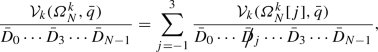 (2.29)
where
 denotes a pinched propagator. This reduction is applied to rank-two objects directly before dressing steps that would otherwise increase the rank to three. In order to avoid the proliferation of new objects, pinched open loops are merged on-the-fly with other open loops stemming from lower-point Feynman diagrams or from other pinched open loops [33]. The numerators in (2.29) have the form $$\begin{aligned} {\mathcal {V}}_k(\varOmega ,\bar{q})&{=} \sum _{s,r} {\mathcal {V}}^s_{k;\mu _1\dots \mu _r}(\varOmega )\, q^{\mu _1}{\cdots } q^{\mu _r}\, ({\tilde{q}}^2)^s, \end{aligned}$$(2.30)
where \(\tilde{q}^2\) terms that arise from pinched propagators (see Sect. 2.4.2) are retained in all UV divergent integrals and lead to \(R_1\) rational terms.

 denotes a pinched propagator. This reduction is applied to rank-two objects directly before dressing steps that would otherwise increase the rank to three. In order to avoid the proliferation of new objects, pinched open loops are merged on-the-fly with other open loops stemming from lower-point Feynman diagrams or from other pinched open loops [
Steps (i)—(iii) are iterated until the loop is entirely dressed.Footnote 9
- (iv)
At this stage, the loops are closed by taking the trace, and the resulting loop integrals,
$$\begin{aligned} \mathcal {W}_{01}(\varOmega )&= \int \!\mathrm {d}^D\!\bar{q}\, \frac{{\mathrm {Tr}}\left[ {\mathcal {V}}(\varOmega , {\bar{q}})\right] }{\bar{D}_{0} \bar{D}_{1}\cdots \bar{D}_{N-1}}, \end{aligned}$$(2.31)are reduced to master integrals upon extraction of \(R_1\) terms, as described at the end of Sect. 2.4.2. Finally, all topologies are summed.
As demonstrated in Sect. 5, the on-the-fly approach yields significant efficiency improvements wrt the original open-loop algorithm. Moreover, based on the one-the-fly reduction algorithm, OpenLoops 2 has been equipped with an automated stability system that cures Gram-determinant instabilities with unprecedented efficiency (see Sect. 2.7).
2.6 Squared loop amplitudes
As outlined in the following, the calculation of squared loop amplitudes (2.3) is organised along the same lines of the parent-child algorithm of Sect. 2.5.1 but with a different colour treatment.
- (i)
The numerators of colour-stripped loop diagrams are constructed with the dressing recursion (2.15) exploiting parent–child relations.
- (ii)
After the last dressing step, loop numerators are closed by taking the trace, and colour-stripped diagrams expressed in terms of integrals \(T_N^{\mu _1\cdots \mu _r}\) (2.18),
$$\begin{aligned} {{\mathcal {A}}}_{1}(\mathcal {I}_N,h)&= \int \!\mathrm {d}^D\!\bar{q}\, \frac{{\mathrm {Tr}}\Big [{\mathcal {N}}({\mathcal {I}}_{N},q,h)\Big ]}{\bar{D}_{0} \bar{D}_{1}\cdots \bar{D}_{N-1}} \nonumber \\&= \sum \limits _{r}\, {\mathrm {Tr}}\Big [\mathcal {N}_{\mu _1\dots \mu _r}(\mathcal {I}_N, h)\Big ]\, T_N^{\mu _1\cdots \mu _r}, \end{aligned}$$(2.32)which are then computed with Collier. While the \(\mathcal {N}_{\mu _1\dots \mu _r}(\mathcal {I}_N, h)\) coefficients need to be evaluated for every helicity state h, the reduction is done only once – and thus very efficiently – at the level of the h-independent tensor integrals.
- (iii)
Individual colour-stripped diagram amplitudes are combined with the corresponding colour structure and converted into colour vectors in the colour basis \(\{{\mathcal {C}}_i\}\),
$$\begin{aligned} \mathcal {M}_1(\mathcal {I}_N,h)&= {\mathcal {C}}(\mathcal {I}_N) \mathcal {A}_1(\mathcal {I}_N,h) \nonumber \\&= \sum _i {\mathcal {C}}_i\,\mathcal {A}^{(i)}_1(\mathcal {I}_N,h). \end{aligned}$$(2.33)Then, summing all diagrams yields the full one-loop colour vector
$$\begin{aligned} \mathcal {A}_1^{(i)}(h)&= \sum _{\mathcal {I}} \mathcal {A}^{(i)}_1(\mathcal {I},h). \end{aligned}$$(2.34) - (iv)
Finally, the helicity/colour summed squared loop amplitude is built though the colour-interference matrix (2.8) as
$$\begin{aligned} \mathcal {W}_{11}&= \frac{1}{N_{\mathrm {hcs}}} \sum _{h}\sum _{\mathrm {col}} \mathcal {M}_1^*(h)\mathcal {M}_1(h) \nonumber \\&= \frac{1}{N_{\mathrm {hcs}}} \sum \limits _{h}\sum \limits _{i,j} K_{ij}\, \big [\mathcal {A}_1^{(i)}(h)\big ]^* \mathcal {A}_1^{(j)}(h). \end{aligned}$$(2.35)
2.7 Numerical stability
The reduction of one-loop amplitudes to scalar integrals suffers from numerical instabilities in exceptional phase-space regions. Such instabilities are related to small Gram determinants of the form
where \(p_k\) are the external momenta in the loop propagators \(D_k\). In regions where rank-two and rank-three Gram determinants become small, the objects that result from the pinching of propagators can be enhanced by spurious \(1/\varDelta \) singularities. At the end, when all pinched objects are combined and the integrals evaluated, such singularities disappear. However, this cancellation can be so severe that all significant digits are lost, and the amplitude output can be inflated in an uncontrolled way by orders of magnitude. This calls for an automated system capable of detecting and curing all relevant instabilities in a reliable way. This is especially important for multi-particle and multi-scale NLO calculations, and even more for NNLO applications, which require high numerical accuracy in regions where one external parton becomes unresolved, thereby inflating spurious poles.
In principle, numerical accuracy can be augmented through quadruple precision (qp) arithmetic. But the resulting CPU overhead, of about two orders of magnitude, is often prohibitive. In OpenLoops, numerical instabilities are thus addressed as much as possible in double precision (dp) using analytic methods. In OpenLoops 1, as detailed below, numerical instabilities are avoided by means of the Collier library [19] in combination with a stability rescue system that makes use of CutTools [10] in qp. In OpenLoops 2, loop-induced processes are handled along the same lines, while standard NLO calculations are carried out with the new on-the-fly reduction algorithm, which is equipped with its own stability system (see Sect. 2.7.2). The latter combines analytic techniques together with a new hybrid-precision system that uses qp in a highly targeted way, requiring only a tiny CPU overhead as compared to a complete qp re-evaluation.
An additional source of numerical instabilities originates from the violation of on-shell relations or total momentum conservation of external particles, i.e. due to the quality of the provided phase-space point. To this end before amplitude evaluation on-shell conditions and momentum conservation are checked. A warning is printed when these conditions are violated beyond a certain relative threshold, which can be altered via the parameter psp_tolerance (\(\hbox {default}=10^{-9}\)). Additionally, we apply a “cleaning procedure” which ensures kinematic constraints of the phase-space up to double precision, rsp. qp where applicable.
2.7.1 Stability rescue system
In the original open-loop algorithm – which was used throughout in OpenLoops 1 and is still used in OpenLoops 2 for squared loop amplitudes and tree–loop interferences in the HEFT – the reduction to scalar integrals is entirely based on external libraries, and the best option is to carry out the reduction of tensor integrals using the Collier library [19]. In the vicinity of spurious poles, Collier cures numerical instabilities by means of expansions in the Gram determinants and alternative reduction methods [4, 34]. Such analytic techniques are applied in a fully automated way, and the resulting level of numerical stability is generally very good. Alternatively, the reduction can be performed at the integrand level using CutTools [10], but this option is mainly used as rescue system in qp, since CutTools does not dispose of any mechanism to avoid instabilities in dp.
In the calculation of tree–loop interferences, numerical instabilities are monitored and cured by means of an automated rescue system based on the following strategy.
- (i)
The stability of tensor integrals is assessed by comparing the two independent Collier implementations of the tensor reduction, Coli-Collier (default) and DD-Collier. This test can be applied to all phase-space points or restricted to a certain fraction of points with the highest virtual K-factorFootnote 10 Given the desired fraction, the points to be tested are automatically selected by sampling the distribution in the K-factor at runtime.
- (ii)
Points that are classified as unstable are re-evaluated in qp using CutTools and OneLOop.
- (iii)
In CutTools, numerical instabilities can remain significant even in qp. Their magnitude is estimated through a so-called rescaling test, where one-loop amplitudes are computed with rescaled masses, dimensionful couplings and momenta and scaled back according to the mass dimensionality of the amplitude.
In this approach, the re-evaluation of the amplitude for stability tests causes a non-negligible CPU overhead. Moreover, additional re-evaluations of the full amplitude in qp are very CPU intensive. Fortunately, thanks to the high stability of Collier, they are typically needed only for a tiny fraction of phase-space points. However, the usage of qp strongly depends on the complexity of the process, and for challenging multi-scale NLO calculations and NNLO applications it can become quite significant.
In the case of squared loop amplitudes, the qp rescue with CutTools is disabled, because of the inefficiency of OPP reduction for loop-squared amplitudes. This is due to the fact that all helicity and colour configurations must be reduced independently. Thus the above stability system is restricted to stage (i). Moreover, due to the fact that a K-factor is not available for loop-squared amplitudes, the comparison of Coli -Collier versus DD -Collier to assess numerical stability is extended to all phase-space points. Details on the usage of the stability rescue system can be found in Sect. 4.6.
2.7.2 On-the-fly stability system
The on-the-fly reduction methods [33] implemented in OpenLoops 2 are supplemented by a new stability system, which is based on the analysis of the analytic structure of spurious singularities in the employed reduction identities. In general, the reduction of loop objects with four or more propagators, \(D_0, D_1, D_2, D_3\dots \), can give rise to spurious singularities in the rank-three Gram determinant \(\varDelta _{123}\), and in the rank-two Gram determinants \(\varDelta _{12}\), \(\varDelta _{13}\) and \(\varDelta _{23}\). In the case of the on-the-fly reduction (2.19), the reduction coefficients associated with a \(D_i\) pinch generate spurious singularities of the form
with a clear hierarchical pattern: very strong instabilities in \(\varDelta _{12}\), mild instabilities in \(\varDelta _{123}\), and no instability in \(\varDelta _{13}\) and \(\varDelta _{23}\). The on-the-fly reduction of objects with only three loop propagators involve only \(\varDelta _{12}\) and yields similar spurious singularities as in (2.37), but without the \(\varDelta _{123}\) term.
Rank-two Gram determinants Instabilities from rank-two Gram determinants are completely avoided in OpenLoops 2. In topologies with four or more propagators, this is achieved via permutations of the loop denominators, \((D_1,D_2,D_3)\rightarrow (D_{i_1},D_{i_2},D_{i_3})\), in the reduction identities. Such permutations are applied on an event-by-event basis in order to guarantee
so that the reduction is always protected from the smallest rank-two Gram determinant.
In this way, rank-two Gram instabilities are delayed to later stages of the reduction, where three-point objects with a single Gram determinant \(\varDelta _{12}\) are encountered. In this case, instabilities at small \(\varDelta _{12}\) are cured by means of an analytic \(\varDelta _{12}\)-expansion, which have been introduced in [33] for the first few orders in \(\varDelta _{12}\) and are meanwhile available to any order [66].
Such expansions have been worked out for those topologies and regions that can lead to \(\varDelta _{12}\rightarrow 0\) in hard scattering processes. This can happen only in t-channel triangle configurations, where two external momenta \(k_1,k_2\) are space-like, and \((k_1+k_2)^2=0\). The relevant virtualities are parametrised as \(k_1^2=-Q^2\) and \(k_2^2=-(1+\delta )Q^2\), where \(Q^2\) is a (high) energy scale, and the Gram determinant is related to \(\delta \) via \(\sqrt{\varDelta _{12}}= Q^2\,\delta /2\). The corresponding three-point tensor integrals are expanded in \(\delta \) based on covariant decompositions of type
where \(L^{\mu _1 \ldots \mu _r}_i\) are Lorentz structures made of metric tensors and external momenta. Their coefficients \(C_i(\delta )\) are reduced to scalar tadpole, bubble and triangle integrals,
i.e.
where \(c^{N}_{i}(\delta )\) are rational functions containing \(1/\delta ^K\) poles, while the \(C_i(\delta )\) coefficients are regular at \(\delta \rightarrow 0\). Numerically stable \(\delta \)-expansions for \(C_i(\delta )\) are obtained via Taylor expansions of the scalar integrals. The required coefficients,
have been determined to any order k in the form of analytic recurrence relations [33] for all mass configurations of type \((m_0,m_1,m_2)=(0, 0, 0)\), (0, m, m), (m, 0, 0), (m, M, M), which cover all possible QCD amplitudes with massless partons and massive top and bottom quarks. Recently, such any-order expansions have been extended to all mass configurations that can occur at NLO EW.Footnote 11
To stabilise the tensor coefficients (2.41), singular terms of the form \(\delta ^{-K}T^N_0(\delta )\) are separated via partial fractioning and replaced by
with
The singular parts cancel exactly when combining the contributions from \(A_0\), \(B_0\) and \(C_0\) functions as well as the rational terms. Thus only the finite series \(T^{N,K}_{0,{\mathrm {fin}}}(\delta )\) need to be evaluated. The fact that all tensor integrals are stabilised using only \(C_0\) and \(B_0\) expansions makes it possible to expand with excellent CPU efficiency up to very high orders in \(\delta \), thereby controlling a broad \(\delta \)-range. In practice, the \(\delta \)-expansions are applied for \(\delta <\delta _{\mathrm {thr}}\), with a threshold \(\delta _{\mathrm {thr}}\) that is large enough to avoid significant instabilities for \(\delta >\delta _{{\mathrm {thr}}}\), while below \(\delta _{{\mathrm {thr}}}\) the expansions are carried out up to a relative accuracy of \(10^{-16}\) (\(10^{-32}\)) in dp (qp). By default \(\delta _{{\mathrm {thr}}}\) is set to \(10^{-2}\).
Rank-three Gram determinants
The on-the-fly reduction coefficients (2.37) associated with \(D_i\) pinches with \(i=1,2,3\) are proportional to \(1/\sqrt{\varDelta _{123}}\) and read [33]
where \(\alpha _i = p_i^2/[p_1 \cdot p_2 (1 + \sqrt{\delta })]\), and \(\ell ^\mu _{1,2,3}\) are auxiliary momenta used to parametrise the loop momentum [33]. In topologies with more than four propagators, \(D_0,D_1, D_2, D_3, D_4,\ldots \), such rank-three Gram instabilities are avoided by performing the reduction in terms of four of the first five propagators, \(D_{i_0} D_{i_1} D_{i_2} D_{i_3}\), which are chosen by first maximising \(|\varDelta _{i_1i_2}|\), to avoid rank-two instabilities, and by subsequently minimising \(\max \{|K_{i_1}|,|K_{i_2}|,|K_{i_3}|\}\). In this way, small rank-three (-two) Gram determinants can largely be avoided until later stages of the recursion, where box (triangle) topologies have to be reduced.
OPP reduction The OPP method, used for five- and higher-point objects of rank smaller than two, is based on the same auxiliary momenta \(\ell _i\) mentioned above. Related rank-two Gram instabilities are avoided by permuting the propagators of the resulting scalar boxes according to (2.38).
IR regions In order to mitigate numerical instabilities in the context of NNLO calculations, OpenLoops implements additional improvements targeted at phase-space regions where one external parton becomes soft or collinear. Such improvements include:
global and numerically stable implementation of all kinematic quantities, including the basis momenta \(\ell ^\mu _i\) used for the reduction, in special regions;
analytic expressions for renormalised self-energies to avoid numerical cancellations between bare self-energies and counterterms in the limit of small \(p^2\). This is relevant for self-energy insertions into propagators that are connected to two external partons via soft or collinear branchings.
Such dedicated treatments for unresolved regions will be documented in [66] and further extended in the future.
Hybrid precision system In order to cure residual instabilities that cannot be avoided with the methods described above, the on-the-fly reduction is equipped with a hybrid-precision (hp) system [66] that monitors all potentially unstable types of reduction identities and switches from dp to qp dynamically when a numerical instability is encountered. This system is fully automated and acts locally, at the level of individual operations. This makes it possible to restrict the usage of qp to a minimal part of the calculation, thereby obtaining a speed-up of orders of magnitude as compared to brute-force qp re-evaluations of the full amplitude. Typically, the extra time spent in qp is only a modest fraction of the standard dp evaluation time. The main features of the hp system are as follows.
Quad precision is triggered and used at the level of individual reduction steps, based on the kinematics of the actual phase-space point and the loop topology of the individual open-loop object that is being processes at a given stage of the recursion.
Reduction steps that are identified as unstable and all consecutive connected operations are carried out in quad precision until spurious singularities are cancelled. Quad precision is thus used for all subsequent operations (dressing, merging, reduction, master integrals) that are connected to an instability.
For each type of reduction step, the magnitude of potential instabilities is estimated based on the actual kinematics and the analytical form of the reduction identity. This information leads to an error estimate that is attributed to each processed object and is propagated and updated through all steps of the algorithm.
Quad precision is triggered when the cumulative error esimate for a certain object exceeds a global accuracy threshold, which can be adjusted by the user (see Sect. 4.6) depending on the required numerical accuracy.
The hp system is based on two parallel dp/qp channels for each generic operation (reduction, dressing, merging) and a twofold dp/qp representation of each object that undergoes such operations. By default the dp channel is used, and when an instability is detected the object at hand is moved to the qp channel, which is used for all its subsequent manipulations. At the end, when spurious singularities are cancelled, qp output is converted back to dp.
The efficiency of the hp system strongly benefits from the above mentioned analytical treatments of Gram determinants and soft regions, which avoid most of the instabilities and delay the remaining ones to later stages of the recursion, minimising the number of subsequent qp steps. As a result, for one-loop calculations with hard kinematics qp is typically needed only for a tiny fraction of the phase-space points, and for a very small part of the calculation of an amplitude. The usage of qp can become significantly more important in NNLO calculations, especially when local subtraction methods are used. In this case, one-loop amplitudes need to be evaluated in deep IR regions, where new types of instabilities occur for which no analytic solution is available at the moment. Such instabilities are automatically detected and cured by the hp system. This may lead, depending on the process and kinematic region, to a significant CPU overhead. In such cases, the accuracy threshold parameter should be tuned such as to achieve an optimal trade-off between performance and numerical stability.
Technical details and usage of the on-the-fly stability system are described in Sect. 4.6.
External libraries Finally, OpenLoops 2 benefits from improvements in Collier 1.2.3 [19], which is used for dp evaluations of scalar integrals and for tensor reduction in loop-induced processes, as well as in OneLOop [65], which is used to evaluate scalar integrals in qp.
3 Automation of tree- and one-loop amplitudes in the full SM
3.1 Power counting
In the Standard Model, scattering amplitudes can be classified based on power counting in the strong and electroweak coupling constants,Footnote 12 \(g_\mathrm {s}=\sqrt{4\pi \alpha _{\mathrm {s}}}\) and \(e=\sqrt{4\pi \alpha }\). At LO in QCD, tree amplitudes have the simple form
where n and m are, respectively, the maximally allowed power in \(g_\mathrm {s}\) and the minimally allowed power in e. The total coupling power is fixed by the number of scattering particles, \(n+m=N_{\mathrm {p}}-2\), where \(N_{\mathrm {p}}\) is the number of scattering particles.
In the SM, the general coupling structure of scattering amplitudes depends on the number \(n_{q\bar{q}}\) of external quark–antiquark pairs. For processes with \(n_{q\bar{q}}\le 1\), the LO QCD term (3.1) is the only tree contribution, while processes with \(n_{q\bar{q}}\ge 2\) involve also sub-leading EW contributions of order \(g_\mathrm {s}^p e^q\) with \(p+q=N_{\mathrm {p}}-2\) and variable power \(q>m\). Such contributions reflect the freedom of connecting quark lines either through EW or QCD interactions. As a result, tree amplitudes consist of a tower of QCD–EW contributions,
where
For \(n_{q\bar{q}}\ge 2\), the Born amplitude (3.2) involves \(n_{q\bar{q}}\) terms, while the squared Born amplitude consists of a tower of \(2n_{q\bar{q}}-1\) terms,
Each term of fixed order in \(\alpha _{\mathrm {s}}\) and \(\alpha \) in (3.4) results from the interference between Born amplitudes of variable order,
where \(s_{\mathrm {min}}=\max (0,r-\tilde{n}_{q\bar{q}})\) and \(s_{\mathrm {max}}=\min (r,\tilde{n}_{q\bar{q}})\). Contributions \(\big \langle \mathcal {M}_0^{(k)}|\mathcal {M}_0^{(k')}\big \rangle \) with \(k'\ne k\) and \(k'=k\) are denoted, respectively, as Born–Born interferences and squared Born terms. The former are typically strongly suppressed with respect to the latter. This is due to the fact that physical observables are typically dominated by contributions involving propagators that are enhanced in certain kinematic regions. Squared amplitudes that involve such propagators are thus maximally enhanced. In contrast, since the propagators of Born amplitudes with \(k'\ne k\) are typically peaked in different regions, Born–Born interferences tend to be much less enhanced. In addition, the interference between diagrams with gluon and photon propagators, which are enhanced in the same regions, turn out to be suppressed as a result of colour interference.

Schematic representation of the towers of mixed QCD–EW terms at LO and NLO. The first row represents the LO tower (3.4)–(3.6), which consists of an alternating series of dominant squared Born terms (dark grey blobs) and sub-leading pure interference terms (light grey blobs). The second row corresponds to the NLO tower (3.14)–(3.24). Each LO term is connected to two NLO terms via QCD (red) and EW (blue) corrections, while each NLO term is connected to a unique squared Born term either via QCD or EW corrections. Apart from the outer most NLO terms of pure QCD and pure EW kind, QCD (EW) corrections to squared Born terms mix with EW (QCD) corrections to adjacent interference terms
Based on these considerations, it is interesting to note that each term (3.5), with fixed order in \(\alpha _{\mathrm {s}}\) and \(\alpha \), contains at most one squared-Born contribution with \(r-s=s\). In fact this is possible only for even values of r. Thus the tower (3.4) consist of an alternating series of \(n_{q\bar{q}}\) squared Born termsFootnote 13 with \(r=2R\),
and \((n_{q\bar{q}}-1)\) pure interference terms with \(r=2R+1\),
The tower of Born terms (3.4) is illustrated in the upper row of Fig. 4. Squared Born terms are shown as large dark grey blobs, while interference terms are depicted as smaller light grey blobs.
At one loop, for processes that are not free from external QCD partons,Footnote 14 the leading QCD contributions have the form
Here NLO QCD should be understood as the \(\mathcal {O}(\alpha _{\mathrm {s}})\) correction wrt the LO QCD term (3.1). For processes with \(n_{q\bar{q}}\ge 2\), the leading QCD terms are accompanied by a tower of sub-leading EW contributions, and the general form of one-loop SM amplitudes is
Here and in the following, the inclusion of all counterterm contributions of UV and \(R_2\) kind as in (2.11) is implicitly understood. One-loop terms of fixed order in \(g_\mathrm {s}\) and e in (3.9) can be regarded either as the result of \(\mathcal {O}(g_\mathrm {s}^2)\) or \(\mathcal {O}(e^2)\) insertions into corresponding Born amplitudes. In this perspective, denoting matrix elements of fixed order as
we can define
where \(\delta _{{\mathrm {QCD}}}\) and \(\delta _{\mathrm {EW}}\) should be understood as operators that transform an \(\mathcal {O}(g_\mathrm {s}^p e^q)\) Born matrix element into the complete one-loop matrix elements of \(\mathcal {O}(g_\mathrm {s}^{p+2} e^q)\) and \(\mathcal {O}(g_\mathrm {s}^p e^{q+2})\), respectively. For processes with \(n_{q\bar{q}}\le ~1\), only one Born term and two one-loop terms exist, and the latter can unambiguously be identified as NLO QCD and NLO EW corrections,
In contrast, processes with \(n_{q\bar{q}}\ge 2\) involve \(\tilde{n}_{q\bar{q}}+1=n_{q\bar{q}}\) terms of variable order \(g_\mathrm {s}^P e^Q\), which can in general be regarded either as QCD corrections to Born terms of relative order \(g_\mathrm {s}^{-2}\) or EW corrections to Born terms of relative order \(e^{-2}\), i.e.
for \(n_{q\bar{q}}\ge 2\). More precisely, one-loop terms with maximal QCD order, \(P_{\max }=n+2\), represent pure QCD corrections, since Born terms of relative order \(e^{-2}\) do not exist. Similarly, one-loop terms of maximal EW order, \(Q_{\max }=m+2+2\tilde{n}_{q\bar{q}}\), are pure EW corrections, since Born terms of relative order \(g_\mathrm {s}^{-2}\) do not exist. In contrast, the remaining \(n_{q\bar{q}}-2\) terms with \(P<P_{\max }\) and \(Q<Q_{\max }\) have a mixed QCD–EW character, in the sense that they involve corrections of QCD and EW type, which coexist at the level of individual Feynman diagrams, such as in loop diagrams where two quark lines are connected by a virtual gluon and a virtual EW boson. This kind of one-loop terms cannot be split into contributions of pure QCD or pure EW type. Thus, in general only the full set of one-loop diagrams containing all mixed QCD–EW terms of order \(g_\mathrm {s}^P e^Q\) represents a well defined and gauge-invariant perturbative contribution. Keeping this in mind, as far as the terminology is concerned, it is often convenient to refer to (3.13) either as QCD correction wrt to \(\mathcal {O}(g_\mathrm {s}^{P-2} e^{Q})\) or EW correction wrt \(\mathcal {O}(g_\mathrm {s}^{P} e^{Q-2})\).
Squaring one-loop amplitudes with \(n_{q\bar{q}}\ge 2\) results in a similar tower of \(2n_{q\bar{q}}-1\) mixed QCD–EW terms as in (3.4)–(3.5). In contrast, the interference of tree and one-loop amplitudes yields a tower of \(2n_{q\bar{q}}\) terms,
Each term of fixed order in \(\alpha _{\mathrm {s}}\) and \(\alpha \) involves the interference between Born and one-loop terms of variable order,
for \(0\le r\le 2\tilde{n}_{q\bar{q}}+1\), where \(t_{\mathrm {min}}=\max (0,r-\tilde{n}_{q\bar{q}})\) and \(t_{\mathrm {max}}=\min (r,\tilde{n}_{q\bar{q}}+1)\).Footnote 15 In general, the one-loop amplitudes that enter (3.15) consist of mixed QCD–EW corrections in the sense of (3.13), i.e.
In practice, as discussed above, the one-loop terms with maximal QCD or maximal EW order consist of pure QCD or pure EW corrections. In (3.14)–(3.15) they correspond to \(r=0\) and \(r=2\tilde{n}_{q\bar{q}}+1\), and they read
and
These contributions are shown as the outer most blobs in the second row of Fig. 4. They emerge as pure \(\mathcal {O}(\alpha _{\mathrm {s}})\) and pure \(\mathcal {O}(\alpha )\) corrections as indicated by the red and blue arrows respectively. The remaining \((2n_{q\bar{q}}-2)\) terms cannot be regarded as pure QCD or pure EW corrections. Nevertheless, due to the fact that the squared Born tower is an alternating series consisting of \(n_{q\bar{q}}\) squared Born terms and \((n_{q\bar{q}}-1)\) pure interference terms, see (3.4)–(3.6), the tree–loop interference (3.14) corresponds to an alternating series of \(n_{q\bar{q}}+n_{q\bar{q}}\) terms that can be interpreted, respectively, as QCD and EW corrections with respect to squared Born terms. Specifically, the terms (3.15) with even indices, \(r=2R\) with \(0\le R\le n_{q\bar{q}}-1\), can be written in the form
where the terms with \(t=R\),
represent QCD corrections to squared Born amplitudes. In contrast, the alternative representation
where \(2R-t \ne t-1\) for all t, shows that EW corrections arise only in connection with interference Born terms, which are typically strongly sub-leading. Vice versa, for terms with odd indices, \(r=2R+1\) with \(0\le R\le \tilde{n}_{q\bar{q}}\), the representation
involves terms with \(t=R+1\),
which represent EW corrections to squared Born amplitudes, while writing
where \(2R+1-t\ne t\) for all t, shows that QCD correction effects enter only through pure interference Born terms and are typically suppressed.
In summary, apart from the leading QCD and EW terms, NLO SM contributions at a given order \(\alpha _{\mathrm {s}}^{n+1-r}\alpha ^{m+r}\) cannot be regarded as pure QCD or pure EW corrections. Nevertheless, the orders \(r=2R\) and \(2R+1\) are typically dominated, respectively, by QCD and EW corrections to the squared Born amplitude \(\mathcal {W}_{00}^{2R}\sim \big \langle \mathcal {M}_0^R|\mathcal {M}_0^R\big \rangle \). Thus, keeping in mind that all relevant EW–QCD mixing and interference effects must always be included, each NLO order can be labelled in a natural and unambiguous way either as QCD or EW correction as illustrated in Fig. 4.
As detailed in Sect. 4.2, OpenLoops supports the calculation of tree and one-loop contributions of any desired order in \(\alpha _{\mathrm {s}}\) and \(\alpha \). In practice, scattering probability densities at different orders in \(\alpha _{\mathrm {s}}\) and \(\alpha \),
are treated as separate subprocesses. Squared Born terms \(\mathcal {W}_{00}^{(p,q)}\) and squared one-loop terms \(\mathcal {W}^{(p,q)}_{11}\) are selected by specifying the QCD order p or the EW order q. Fixing q selects also the related NLO QCD tree–loop interferences, \(\mathcal {W}_{01}^{(p+1,q)}\), while fixing p yields their NLO EW counterpart, \(\mathcal {W}_{01}^{(p,q+1)}\). Alternatively, tree-loop interferences of order \(\alpha _{\mathrm {s}}^P\alpha ^Q\) can be selected directly through the corresponding one-loop powers P or Q.
3.2 Input schemes and parameters
In this section we discuss the different input schemes and the SM input parameters that are used for the calculation of scattering amplitudes in OpenLoops. All parameters are initialised with physical default values, and can be adapted by the user by calling the Fortran routine set_parameter or the related C/ functions as detailed in Appendix A.2. Table 10 in Appendix C summarises input parameters and switchers that can be controlled through set_parameter. Parameters with mass dimension should be entered in GeV units. The values of specific parameters in OpenLoops can be obtained by calling the routine get_parameter, and the full list of parameter values can be printed to a file by calling the function printparameter (see Appendix A.2).
Masses and widths The OpenLoops parameters mass(PID) and width(PID) correspond, respectively, to the on-shell mass \(M_i\) and the width \(\varGamma _i\) of the particle with PDG particle number PID (see Table 6). Masses and widths are treated as independent inputs. For unstable particles, when \(\varGamma _i>0\), the complex-mass scheme [38] is used. In this approach, particle masses are replaced throughout by the complex-valued parameters
This guarantees a gauge-invariant description of resonances and related off-shell effects. By default, \(\varGamma _i=0\) and \(\mu _i = M_i \in {\mathbb {R}}\) for all SM particles, i.e. unstable particles are treated as on-shell states, while setting \(\varGamma _i> 0\) for one or more unstable particles automatically activates the complex-mass scheme for the particles at hand. By default, \(M_i>0\) only for \(i=W,Z,H,t\).
For performance reasons, the public OpenLoops libraries are typically generated with \(m_e=m_\mu =m_\tau =0\) and \(m_u=m_d=m_s=m_c=0\), while generic mass parameters \(m_q\) are used for the heavy quarks \(q=b,t\). By default, heavy-quark masses are set to \(m_b=0\) and \(m_t=172\) GeV, but their values can be changed by the user as desired. Dedicated process libraries with additional fermion-mass effects (any masses at NLO QCD and finite \(m_\tau \) at NLO EW) can be easily generated upon request. For efficiency reasons, when \(m_Q\) is set to zero for a certain heavy quark, whenever possible amplitudes that involve Q as external particle are internally mapped to corresponding (faster) massless amplitudes. To this end the desired fermion masses have to be specified before any process is registered, see Sect. 4.2.
Strong coupling The values of \(\alpha _{\mathrm {s}}(\mu _\mathrm{R}^2)\) and the renormalisation scale \(\mu _\mathrm{R}\) can be controlled through the parameters alphas and muren, respectively. These parameters can be set dynamically on an event-by-event basis,Footnote 16 and OpenLoops 2 implements a new automated scale-variation system that makes it possible to evaluate the same scattering amplitude at multiple values of \(\mu _\mathrm{R}\) and/or \(\alpha _{\mathrm {s}}(\mu _\mathrm{R}^2)\) with high efficiency (see Sect. 4.3).
Number of colours By default, in OpenLoops colour effects and related interferences are included throughout, i.e. scattering amplitudes are evaluated by retaining the exact dependence on the number of colours \(N_c\). In addition, dedicated process libraries with large-\(N_c\) expansions can be generated by the authors upon request. When available, leading-colour amplitudes can be selected at the level of process registration (see Sect. 4.2) via the parameter \(\texttt {leading\_colour}=1\) (default=0).
EW gauge couplings The U(1) and SU(2) gauge couplings \(g_1, g_2\) are derived from
where \(e=\sqrt{4\pi \alpha }\) and \(\theta _{\mathrm {w}}\) denotes the weak mixing angle. The latter is always defined through the ratio of the weak-boson masses [68],
If \(\varGamma _{W}=\varGamma _Z=0\), then \(\cos \theta _{\mathrm {w}}=M_{W}/M_Z\) is real valued. But in general the mixing angle is complex valued. For the electromagnetic coupling three different definitions are supported:
- (i)
\(\varvec{\alpha (0)}\)-scheme: as input for \(\alpha \) the parameter alpha_qed_0 is used, which corresponds to the QED coupling in the \(Q^2\rightarrow 0\) limit. This scheme is appropriate for pure QED interactions at scales \(Q^2\ll M_{W}^2\), and for the production of on-shell photons (see below).
- (ii)
\({\varvec{G}}_{{\varvec{\mu }}}\)-scheme: the input value of \(\alpha \) is derived from the matching condition
$$\begin{aligned} \Big \vert \frac{8}{\sqrt{2}} G_{\mu }\Big \vert ^2 = \Big \vert \frac{g_2^2}{\mu _W^2} \Big \vert ^2, \end{aligned}$$(3.29)which relates squared matrix elements for the muon decay in the Fermi theory to corresponding W-exchange matrix elements in the low-energy limit. This results intoFootnote 17
$$\begin{aligned} \alpha \vert _{G_{\mu }}= \frac{\sqrt{2}}{\pi } \, G_{\mu }\Big \vert \mu _W^2 \sin ^2\theta _{\mathrm {w}}\Big \vert . \end{aligned}$$(3.30)As input for \(\alpha \vert _{G_{\mu }}\) the parameter Gmu is used, which corresponds to the Fermi constant \(G_{\mu }\). The \(G_{\mu }\)-scheme resums large logarithms associated with \(\alpha (M_Z^2)\) as well as universal \(M_t^2/M_W^2\) enhanced corrections associated with the \(\rho \) parameter. This guarantees an optimal description of the strength of the SU(2) coupling, i.e. W-interactions, at the EW scale.
- (iii)
\({\varvec{\alpha }}{\varvec{(}}{{\varvec{M}}}_{{\varvec{Z}}}^{\mathbf{2}}{\varvec{)}}\)-scheme: as input for \(\alpha \) the parameter alpha_qed_mz is used, which corresponds to the QED coupling at \(Q^2=M_Z^2\). This scheme is appropriate for hard EW interactions around the EW scale, where it guarantees an optimal description of the strength of QED interactions and a decent description of the strength of weak interactions.
The choice of \(\alpha \)-input scheme is controlled by the OpenLoops parameter ew_scheme as detailed in Table 1, where also the default input values are specified. Note that \(\alpha (0)\) and \(\alpha (M_Z^2)\) are described by means of two distinct parameters in OpenLoops. Depending on the selected scheme, the appropriate parameter should be set.
External photons The high-energy couplings \(\alpha \vert _{G_{\mu }}\) and \(\alpha (M_Z^2)\) are appropriate for the interactions of EW gauge bosons with virtualities of the order of the EW scale. In contrast, the appropriate coupling for external high-energy photons is \(\alpha (0)\) [70]. More precisely, for photons of virtuality \(Q_\gamma ^2\) the coupling \(\alpha (Q_\gamma ^2)\) should be used. For initial- or final-state on-shell photons this corresponds to \(\alpha (0)\). However, in photon-induced hadronic collisions, initial-state photons inside the hadrons effectively couple as off-shell partons with virtuality \(Q^2_\gamma = \mu _F^2\), where \(\mu _\mathrm{F}\) is the factorisation scale of the parton distribution functions (see Appendix A.3 of [36]), Thus, at high \(\mu _F^2\) the high-energy couplings \(\alpha \vert _{G_{\mu }}\) or \(\alpha (M_Z^2)\) should be used.
Based on these considerations, for processes with n on-shell and \(n_*\) “off-shell” hard external photons plus a possible unresolved photon,
the scattering probability densities \(\mathcal {W}=\mathcal {W}_{00},\mathcal {W}_{01},\mathcal {W}_{11}\) are automatically rescaled asFootnote 18
with LSZ-like coupling correction factors
Here \(\alpha \) should be understood as the QED coupling in the input scheme selected by the user, while the value of \(\alpha (0)\) correspond to the parameter \(\texttt {alpha\_qed\_0}\) and is independent of the scheme choice. The coupling of off-shell external photons and the resulting \(R^{({\mathrm {off}})}_\gamma \) factor are set internally as
which implies
In this way \(\alpha _{\mathrm {off}}\) is guaranteed to be a high-energy coupling. Note that unresolved photons, i.e. additional photons emitted at NLO EW, need to be treated in a different way. In this case, in order to guarantee the correct cancellation of IR singularities, real and EW corrections should be computed with the same QED coupling. This implies that the coupling \(\alpha \) of unresolved photons should not receive any \(R_\gamma \) rescaling.
The relevant information to determine the number of on-shell and off-shell external photons in (3.32) should be provided by the user on a process-by-process basis. To this end, when registering a process with external photons (see Sect. 4.2), unresolved photons should be labelled with the standard PDG identifier PID = 22, while for on-shell and off-shell hard photons, respectively, PID = 2002 and PID = \(-2002\) should be used. In order to guarantee an optimal choice of \(\alpha \), external photons should be handled according to the following classification.
Unresolved photons (iPDG = 22): extra photons (absent at LO) in NLO EW bremsstrahlung.
Hard photons of on-shell type (iPDG = 2002): standard hard final-state photons that do not undergo \(\gamma \rightarrow f{\bar{f}}\) splittings at NLO EW, or initial-state photons at photon colliders;
Hard photons of off-shell type (iPDG \(= -2002\)): hard final-state photons that undergo \(\gamma \rightarrow f{\bar{f}}\) splittings at NLO EW, or initial-state photons from QED PDFs in high-energy hadronic collisions.
Here “hard” should be understood as the opposite of “unresolved”, i.e. it refers to all photons that are present as external particles starting from LO.
By default, the \(R^{({\mathrm {on}})}_\gamma \) and \(R^{({\mathrm {off}})}_\gamma \) rescaling factors in (3.32)–(3.33) are applied to all on-shell and off-shell photons. They can be deactivated independently of each other by setting, respectively, onshell_photons_lsz=0 (default=1) and offshell_photons_lsz=0 (default=1).
Yukawa and Higgs couplings The interactions of Higgs bosons with massive fermions is described by the Yukawa couplings
Here v corresponds to the vacuum expectation value, while \({\mu }_{f,{\mathrm {Y}}}\) is a Yukawa mass parameter. At LO and NLO QCD, the complex-valued Yukawa masses can be freely adapted through the parameters yuk(PID) and yukw(PID), which play the role of real Yukawa masses \({M}_{i,{\mathrm {Y}}}\) and widths \({\varGamma }_{i,{\mathrm {Y}}}\). More explicitly, in analogy with (3.26),
At NLO QCD, as discussed in Sect. 3.3.1, Yukawa couplings can be renormalised in the \(\overline{\text {MS}}\) scheme or, alternatively, as on-shell fermion masses.
By default, according to the SM relation between Yukawa couplings and masses, the Yukawa masses \({\mu }_{f,{\mathrm {Y}}}\) are set equal to the complex masses \(\mu _f\) in (3.26). More precisely, each time that mass(PID) and width(PID) are updated, the corresponding Yukawa mass parameters yuk(PID) and yukw(PID) are set to the same values. Thus, modified Yukawa masses should always be set after physical masses. This interplay, can be deactivated by setting \(\texttt {freeyuk\_on}=1\) (\(\hbox {default}=0\)). In this case, yuk(PID) and yukw(PID) are still initialised with the same default values as mass parameters, but are otherwise independent. This switcher acts in a similar way on the Yukawa renormalisation scale \(\mu _{f,{\mathrm {Y}}}\) in (3.52). At NLO EW, modified Yukawa masses are not allowed.Footnote 19
The triple and quartic Higgs self-couplings are implemented as
where \(\mu _H\) denotes the Higgs mass. By default \(\kappa ^{(3,4)}_{H}=1\), consistently with the SM. At NLO QCD, and also at NLO EW for processes that are independent of \(\lambda _H^{(3,4)}\) at tree level, the Higgs self-couplings can be modified through the naive real-valued rescaling parameters \(\texttt {lambda\_hhh}\equiv \kappa ^{(3)}_{H}\) and \(\texttt {lambda\_hhhh}\equiv \kappa ^{(4)}_{H}\).
Wherever present, the imaginary parts of \(\mu _f\), \(\mu _H\), \(\mu _W\) and \(\sin \theta _{\mathrm {w}}\) are consistently included throughout in (3.36)–(3.38).
Higgs effective couplings Effective Higgs interactions in the \(M_t\rightarrow \infty \) limit are parametrised in such a way that the Feynman rule for the vertices with two gluons and n Higgs bosons read
where
and \(p_1\), \(p_2\) are the incoming momenta of the gluons. The power counting in the coupling constants is done in e and \(g_\mathrm {s}\) as in the SM. In the Higgs Effective Field Theory, only QCD corrections are currently available.
CKM matrix The OpenLoops program can generate scattering amplitudes with a generic CKM matrix \(V_{ij}\). However, for efficiency reasons, most process libraries are generated with a trivial CKM matrix, \(V_{ij}=\delta _{ij}\). Process libraries with a generic CKM matrix are publicly available for selected processes, such as charged-current Drell-Yan production in association with jets, and further libraries of this kind can be generated upon request. When available, such libraries can be used by setting \(\texttt {ckmorder=1}\) before the registration of the process at hand (see Sect. 4.2). In this case the default values of \(V_{ij}\) remain equal to \(\delta _{ij}\), but the real and imaginary parts of the CKM matrix can be set to any desired value by means of the input parameters VCKMdu, VCKMsu, VCKMbu, VCKMdc, VCKMsc, VCKMbc, VCKMdt, VCKMst, VCKMbt for \({\mathrm {Re}}(V_{ij})\) and VCKMIdu, VCKMIsu, etc. for \({\mathrm {Im}}(V_{ij})\).
3.3 Renormalisation
Divergences of UV and IR type are regularised in \(D=4-2{\varepsilon }\) dimensions and are expressed as poles of the form \(C_\epsilon \, \mu _{D}^{2{\varepsilon }}/{\varepsilon }^{n}\), where \(\mu _{D}\) is the scale of dimensional regularisation, and
is the conventional \(\overline{\text {MS}}\) normalisation factor. For a systematic bookkeeping of the different kinds of divergences, UV and IR poles are parametrised in terms of independent dimensional factors (\({\varepsilon }_{\mathrm {UV}},{\varepsilon }_{\mathrm {IR}}\)) and scales (\(\mu _{\mathrm {UV}},\mu _{\mathrm {IR}}\)). Thus, one-loop matrix elements involve three types of poles,
Renormalised one-loop amplitudes computed by OpenLoops are free of UV divergences. Yet, bare amplitudes with explicit UV poles can also be obtained (see Sect. 4.3). The remaining IR divergences are universal and can be cancelled through appropriate subtraction terms (see Sect. 3.4).
For the renormalisation of UV divergences we apply the following generic transformations of masses, fields and coupling parameters,
where \(\mu ^2_{i,0}\), \(\varphi _{i,0}\), \(g_{i,0}\) denote bare quantities, and \(\delta \mu _i^2\), \(\delta Z_{\varphi _i \varphi _j}\), \(\delta Z_{g_i}\) the respective counterterms.
For unstable particles, as discussed in Sect. 3.3.2, OpenLoops implements a flexible combination of the on-shell scheme [37] and the complex-mass scheme [38]. In this approach, the width parameters \(\varGamma _i\) of the various unstable particles can be set to non-zero or zero values independently of each other. Depending on this choice, the corresponding particles are consistently renormalised as resonances with complex masses or as on-shell external states with real masses.
In the following, we discuss the various counterterms needed at NLO QCD and NLO EW. In general, as discussed in Sect. 3.1, one-loop contributions of \(\mathcal {O}(\alpha _{\mathrm {s}}^P\alpha ^Q)\) can require \(\mathcal {O}(\alpha _{\mathrm {s}})\) counterterm insertions in Born terms of \(\mathcal {O}(\alpha _{\mathrm {s}}^{P-1}\alpha ^Q)\) as well as \(\mathcal {O}(\alpha )\) counterterm insertions in Born terms of \(\mathcal {O}(\alpha _{\mathrm {s}}^{P}\alpha ^{Q-1})\).
3.3.1 QCD renormalisation
The SM parameters that involve one-loop counterterms of \(\mathcal {O}(\alpha _{\mathrm {s}})\) are the strong coupling, the quark masses, and the related Yukawa couplings.
Strong coupling The renormalisation of the strong coupling constant is carried out in the \(\overline{\text {MS}}\) scheme, and can be matched in a flexible way to the different flavour-number schemes that are commonly used in NLO QCD calculations. To this end, the full set of light and heavy quarks that contribute to one-loop amplitudes and counterterms is split into a subset of active quarks (\(q\in {\mathcal {Q}}_{\mathrm {active}}\)) and a remaining subset of decoupled quarks (\(q\notin {\mathcal {Q}}_{\mathrm {active}}\)). Active quarks with mass \(m_q\ge 0\) are assumed to contribute to the evolution of \(\alpha _{\mathrm {s}}(\mu _\mathrm{R}^2)\) above threshold. Thus they are renormalised via \(\overline{\text {MS}}\) subtraction at the scale \(\mu =\max (\mu _\mathrm{R},m_q)\). The remaining heavy quarks (\(q\notin {\mathcal {Q}}_{\mathrm {active}}\)) are assumed to contribute only to loop amplitudes and counterterms, but not to the running of \(\alpha _{\mathrm {s}}(\mu _\mathrm{R}^2)\). Thus, they are renormalised in the so-called decoupling scheme, which corresponds to a subtraction at zero momentum transfer.
The explicit form of the \(g_\mathrm {s}\) counterterm reads
where \(C_A=3\) and \(T_F=1/2\), while \(\mu _\mathrm{R}\) and \(\mu _{\mathrm {UV}}\) are the renormalisation and dimensional regularisation scales for UV divergences, respectively. The logarithmic terms associated with quark loops read

The number of active and decoupled quarks included in (3.46) is determined as explained in the following.
Choice of flavour-number scheme In NLO QCD calculations, the logarithms of \(\mu _\mathrm{R}\) in the counterterm (3.46)–(3.47) should cancel the leading-order \(\mu _\mathrm{R}\) dependence associated with \(\alpha _{\mathrm {s}}(\mu _\mathrm{R}^2)\). To this end, the number \(N_{q,{\mathrm {active}}}\) of active quark flavours in (3.46) should be set equal to the number \(N_{\mathrm {F}}\) corresponding to the flavour-number scheme of the calculation at hand. More precisely, when using a running \(\alpha _{\mathrm {s}}(\mu _\mathrm{R}^2)\) with \(N_{\mathrm {F}}\) quark flavours, the userFootnote 20 should set \(N_{q,{\mathrm {active}}}=N_{\mathrm {F}}\). In variable-flavour number schemes, \(N_{\mathrm {F}}\) corresponds to the maximum number of quark flavours in the evolution, and typically \(N_{\mathrm {F}}=4,5\) or 6.Footnote 21
In practice, the number of active quarks in OpenLoops is determined as
where \(N_{\mathrm {F}}\) corresponds to the desired flavour-number scheme and can be specified by the user through the parameter \(\texttt {nf}{} \texttt {\_}{} \texttt {alphasrun}\), while \(N_{q,m=0}\) is determined from the number of quarks with \(m_q=0\) at runtime. By default \(\texttt {nf}{} \texttt {\_}{} \texttt {alphasrun=0}\), and all massless quarks are treated as active, while massive quarks are decoupled. In contrast, if \(\texttt {nf}{} \texttt {\_}{} \texttt {alphasrun}\) is set to a value \(N_{\mathrm {F}}>N_{q,m=0}\), the first \(N_{\mathrm {F}}\) massless or massive quarks are treated as active above threshold, and only the remaining heavy quarks are decoupled. For example, when \(m_b=0\) the default value of \(N_{q,{\mathrm {active}}}\) is 5, and \(\texttt {nf\_alphasrun}\) should be set to 6 in case a 6-flavour \(\alpha _{\mathrm {s}}\) is used. In contrast, for \(m_b\ne 0\) the default value of \(N_{q,{\mathrm {active}}}\) is 4, and \(\texttt {nf\_alphasrun}\) should be set to \(N_{\mathrm {F}}\) in case a \(N_{\mathrm {F}}\)-flavour \(\alpha _{\mathrm {s}}\) with \(N_{\mathrm {F}}>4\) is used.
Total number of quark flavours By default, most public OpenLoops libraries involve quark-loop contributions with \(N_{q,{\mathrm {loop}}}=6\) quark flavours. Such libraries can be used for NLO calculations in any flavour-number scheme with \(N_{\mathrm {F}}=N_{q,{\mathrm {loop}}}\) or \(N_{\mathrm {F}}<N_{q,{\mathrm {loop}}}\). In the latter case, heavy-quark loop contributions that do not contribute to the evolution of \(\alpha _{\mathrm {s}}(\mu _\mathrm{R}^2)\) are consistently accounted for by the \(N_{q,{\mathrm {loop}}}-N_{\mathrm {F}}\) decoupled quarks in the one-loop matrix elements.
Extra libraries without top-quark loops (\(N_{q,{\mathrm {loop}}}=5\)) can be easily generated upon request and are publicly available for selected processes. When available, libraries with \(N_{q,{\mathrm {loop}}}<6\) can be used by setting the parameter \(\texttt {nf}\) (default=6) to the desired value of \(N_{q,{\mathrm {loop}}}\) at the moment of the process registration.
Quark masses At NLO QCD, quark masses can be renormalised in the on-shell scheme (default) or in the \(\overline{\text {MS}}\) scheme. The general form of mass counterterms is
where \(C_F=3/4\), and logarithms of the complex mass \(\mu _q\) are complex valued when \(\varGamma _q>0\). The scheme- dependent finite part reads

Here \(\varLambda _{q}\) denotes the \(\overline{\text {MS}}\) renormalisation scale for the mass of the quark q. This scale is controlled by the (real-valued) parameter LambdaM(PID), which plays also the role of scheme setter for the mass counterterm of the quark at hand. For \(\varLambda _{q}=0\) (default) the on-shell scheme is used, while setting \(\varLambda _{q}>0\) activates the \(\overline{\text {MS}}\) scheme.
Yukawa couplings According to (3.36), Yukawa couplings are defined in terms of related Yukawa masses. Their ratio \({\mu }_{q,{\mathrm {Y}}}/\lambda _q=v/\sqrt{2}\) depends only on the vacuum expectation value, which does not receive \(\mathcal {O}({\alpha _{\mathrm {s}}})\) corrections. This implies the trivial counterterm relation
Similarly as for the quark masses \(\mu _q\), also Yukawa masses can be renormalised on-shell (default) or via \(\overline{\text {MS}}\) subtraction. The counterterms read
with \(X(\mu _{q,{\mathrm {Y}}},\varLambda _{q,{\mathrm {Y}}})\) as defined in (3.50). The \(\overline{\text {MS}}\) renormalisation scale \(\varLambda _{q,{\mathrm {Y}}}\) for the Yukawa mass of the quark q is controlled by the independent parameter LambdaY(PID). By default \(\varLambda _{q,{\mathrm {Y}}}=0\), and the on-shell counterterm is used, while setting \(\varLambda _{q,{\mathrm {Y}}}>0\) activates the \(\overline{\text {MS}}\) renormalisation. Similarly as for Yukawa masses (3.37), the values of \(\varLambda _{q,{\mathrm {Y}}}\) are automatically synchronised with \(\varLambda _{q}\) when the latter is changed, but not vice versa. Thus the order in which LambdaM(PID) and LambdaY(PID) are set matters. As for Yukawa masses, this interplay can be deactivated by setting freeyuk_on=1 (\(\hbox {default}=0\)).
Wave functions The QCD counterterms for gluon and quark wave functions read
and
where \(\mu _{\mathrm {IR}}\) is the dimensional regularisation scale for IR divergences, \(\varTheta (M)\) is the step function with \(\varTheta (0)=0\), and
Higgs effective couplings The QCD counterterm associated with the Higgs effective vertex (3.39)–(3.40) reads
where the last term originates from the two-loop matching of the Higgs effective coupling [71, 72]. For double- (and multi-) Higgs production at the same order as the NLO QCD corrections also double-operator insertions with the same total number of Higgs bosons contribute. In OpenLoops these contributions are automatically included as pseudo-counterterms together with the virtual amplitudes.
Renormalisation and regularisation scales At the level of the user interface, the UV and IR regularisation scales are treated as a common scale \(\mu _{D}=\mu _{\mathrm {UV}}=\mu _{\mathrm {IR}}\), and the logarithms of \(\mu _{\mathrm {UV}}^2/\mu _{\mathrm {IR}}^2\) in (3.55) are set to zero. In the literature, also the logarithms of \(\mu _{\mathrm {UV}}^2/\mu _\mathrm{R}^2\) in (3.46)–(3.47) are often omitted by assuming \(\mu _{\mathrm {UV}}=\mu _\mathrm{R}\) in the \(\overline{\text {MS}}\) scheme. On the contrary, in OpenLoops the values of \(\mu _{D}\) and \(\mu _\mathrm{R}\) are controlled by two independent parameters, mureg and muren, respectively. Their default values are \(\mu _{D}=\mu _\mathrm{R}=100\) GeV. For convenience it is possible to simultaneously set \(\mu _\mathrm{R}=\mu _{D}=\mu \) by means of the auxiliary OpenLoops parameter mu. As described in Sect. 4.3, variations of \(\mu _\mathrm{R}\) and \(\alpha _{\mathrm {s}}(\mu _\mathrm{R}^2)\) can be carried out in a very efficient way in OpenLoops 2.
3.3.2 EW renormalisation
The renormalisation of UV divergences in the EW sector is based on the scheme of [37] for on-shell particles, and on the complex-mass scheme [38] for the treatment of off-shell unstable particles. In OpenLoops 2 these two schemes are combined into a flexible renormalisation scheme that makes it possible to deal with processes such as \(pp\rightarrow t {\bar{t}} \ell ^+ \ell ^-\), where some unstable particles (\(t,{\bar{t}}\)) are treated as on-shell external states, while other ones (Z) play the role of intermediate resonances. This is achieved through a refined definition of field-renormalisation constants, and by adapting the mass-renormalisation prescriptions for unstable particles on a particle-by-particle basis, depending on whether the individual width parameters \(\varGamma _i\) are set to non-zero values or not by the user. As explained in the following, the \(\mathcal {O}(\alpha )\) renormalisation in OpenLoops involves also a non-standard treatment of \(\varDelta \alpha (M_Z^2)\) and special features related to external photons.
Counterterms for complex masses The propagators of unstable particles with \(\varGamma _i\ne 0\) are renormalised in the complex-mass scheme [38], where the renormalised self-energy is defined as
The counterterm \(\delta \mu _i^2\) associated with the complex mass (3.26) corresponds to a subtraction of the full complex-valued self-energy at \(p^2=\mu _i^2\). In particular, the counterterm \(\delta \mu ^2_i\) includes also the imaginary part of the self-energy, which is related to the width through
and is already included in the imaginary part of \(\mu ^2_i\). Thus the subtraction of \({\mathrm {Im}}\,\varSigma \) in the complex-mass scheme is mandatory in order to avoid double counting. Since the renormalised self-energy (3.57) vanishes at \(p^2\rightarrow \mu _i^2\), the tree-level and one-loop propagators have the same resonant form \(1/(p^2-M_i^2+\mathrm {i}\varGamma _i M_i)\), where width effects are controlled by the user-defined width parameter \(\varGamma _i\).
For convenience, the relevant 2-point integrals with complex-valued momenta \(p^2=\mu ^2_i=M^2-\mathrm {i}\varGamma _i M_i\) can be obtained through a first-order expansion in \(\varGamma _i/M_i\) around \(p^2=M_i^2\) [38]. In this context, self-energy graphs involving massless photons require a special treatment due to the presence of a threshold at \(p^2=\mu ^2\). In this case, the correct expansion of the scalar two-point function reads
where the additional \(-\mathrm {i}\varGamma /M\) term accounts for the non-analytic behaviour at \(p^2=\mu ^2\). The related expansion formula for generic self-energies reads
where the non-analytic expansion coefficient is given by
and depends only on the electromagnetic charge \(Q_i\) of the particle at hand. This is due to the fact that (3.61) originates only from photon-exchange diagrams and is related to the presence of an infrared singularity in \(B_0'\) at \(p^2\rightarrow \mu _i^2\).
The expanded mass counterterms for Higgs (\(i=H\)) and vector bosons (\(i=V=W,Z\)) read
and
where \(\varSigma _{\mathrm {T}}\) denotes the transverse part of the gauge-boson propagator. The renormalisation of fermion masses depends on the following combination of left-handed (L), right-handed (R) and scalar (S) self-energy contributions,
and the expanded counterterm reads
Counterterms for real masses When \(\varGamma _i\) is set to zero, unstable and stable particles are described as on-shell states with a real-valued mass parameter, \(\mu _i=M_i\). In this case a conventional on-shell renormalisation is applied,
with
Here the subtraction is restricted to the real part of the self-energy, while the \({\mathrm {Im}}\,\varSigma \) contribution must be retained, since it is not included in the renormalised parameter \(M_i^2\). More precisely, the \({\widetilde{{\mathrm {Re}}}}\) operator in (3.66) truncates only the imaginary parts associated with the UV-finite absorptive parts of two-point integrals,Footnote 22 while, in order to ensure a consistent cancellation of UV divergences, all other imaginary parts associated with complex-valued couplings or complex masses inside the loop are kept throughout. The explicit on-shell mass counterterms for Higgs or vector bosons and fermions read
Yukawa couplings At NLO EW, Yukawa couplings (3.36) are always related to fermion masses as predicted by the SM. Thus Yukawa masses and physical fermion masses, as well as the respective counterterms, are equal to each other. This implies
For the renormalisation of the fermion masses \(\mu _f\) only the on-shell scheme, or its complex-mass scheme variant, are supported.
Wave functions The wave-function renormalisation constants (WFRCs) \(\delta Z_{ij}\) are defined in a way that one-loop propagators do not mix, and their residues are normalised to one. Thus renormalised amplitudes correspond directly to S-matrix elements and do not require additional LSZ factors. On the one hand, due to the presence of absorptive contributions and complex parameters, in the complex-mass scheme the \(\delta Z_{ij}\) constants can acquire complex values. On the other hand, the WFRCS for on-shell particles are usually defined as real parameters [37]. As explained in detail below, in OpenLoops these two approaches are reconciled by implementing WFRCs in a way that is consistent with [37] when the width parameters \(\varGamma _i\) are set to zero for all particles, while imaginary \(\delta Z_{ij}\) contributions are taken into account wherever they are strictly needed for the consistency of the complex-mass scheme at \(\mathcal {O}(\alpha )\).
At NLO, the renormalisation of the field \(\varphi _i\) associated with a certain external leg yields
Since the imaginary parts of the diagonal WFRCs \(\delta Z_{ii}\) contribute only at \(\mathcal {O}(\alpha ^2)\), in OpenLoops we omit them by defining
In contrast, the non-diagonal WFRCs associated with \(\gamma \)–Z mixing are defined as
where \(\varSigma _\mathrm {T}^{AZ}(Q^2)\) denotes the transverse part of the \(\gamma \)–Z mixing energy. Here the imaginary part of \(\mu _Z\) in the denominator is retained in order to ensure UV cancellations in the complex-mass scheme, while absorptive parts are truncatedFootnote 23 in order to match the conventional on-shell scheme when all \(\varGamma _i\) are set to zero. For \(\delta Z_{AZ}\) the mixing energy at \(p^2=\mu _Z^2\) is expressed through an expansion around \(p^2=M_Z^2\) neglecting terms of \(\mathcal {O}(\varGamma ^2/M^2)\). However, in practice this expansion is irrelevant, since \(\delta Z_{AZ}\) only contributes for processes with external Z-bosons, where \(\varGamma _Z=0\) is required.
At NLO EW, the independent renormalisation of left- and right-chiral fields corresponds to a diagonal renormalisation matrix in chiral space,
For massless fermions, the matrix (3.79) is diagonal also in helicity space, and imaginary parts can be amputated similarly as for the diagonal WFRCs (3.76). In contrast, for massive fermions the matrix (3.79) mixes left- and right-handed helicity states. Thus, in this case imaginary parts are treated in a similar way as for the non-diagonal WFRCs (3.77). Thus the explicit form of the fermionic WFRCs \(\delta Z_{f_{\mathrm {R},\mathrm {L}}}\) reads
Variations of the complex-mass scheme Certain aspects of the complex-mass scheme at \(\mathcal {O}(\alpha )\) can be changed using the parameter complex_mass_scheme as detailed in the following.
- (i)
complex_mass_scheme=1 (default) corresponds to the implementation described above: the complex-mass counterterms (3.62)–(3.65) are used when \(\varGamma _i>0\), and the on-shell mass counterterms (3.71)–(3.73) are used when \(\varGamma _i=0\), while for WFRCs the generic formulas (3.76)–(3.80) are applied. As discussed above, this flexible approach guarantees a consistent one-loop description of processes like \(pp\rightarrow t {\bar{t}} \ell ^+ \ell ^-\), where unstable particles occur both as internal resonances and as on-shell external states.
- (ii)
complex_mass_scheme=0 keeps the complex masses (3.26) unchanged but deactivates the complex-mass scheme at the level of all \(\mathcal {O}(\alpha )\) counterterms: for mass counterterms the on-shell formulas (3.71)–(3.73) are used throughout; moreover, the \({\widetilde{{\mathrm {Re}}}}\) operations in (3.71)–(3.73) and (3.76)–(3.80) are replaced by a complete truncation of the imaginary parts at the level of the full counterterms. This option is implemented for validation purposes. Depending on the process, it can result in incomplete pole cancellations or other inconsistencies, in particular when internal or external particles with \(\varGamma _i>0\) are present.
- (iii)
complex_mass_scheme=2 corresponds to the implementation of the complex-mass scheme in Recola [20]. In this case all mass counterterms are evaluated with the complex-mass scheme formulas (3.62)–(3.65), while all \({\mathrm {Re}}\) and \({\widetilde{{\mathrm {Re}}}}\) operators are removed from (3.76)–(3.80), i.e. all imaginary parts of WFRCs are kept exact.
Light-fermion contributions to \(\varDelta \alpha (M_Z^2)\) The \(\mathcal {O}(\alpha )\) corrections to processes with on-shell external photons involve the renormalisation constant \(\delta Z_{AA}\) defined in (3.76), which is related to the photon vacuum polarisation \(\varPi ^{\gamma \gamma }(Q^2)\) at \(Q^2\rightarrow 0\) via
Terms involving \(\varPi ^{\gamma \gamma }(0)\) occur also in the \(\alpha (0)\) counterterm (3.87), which contributes to any process that is parametrised in terms of \(\alpha (0)\) at tree level. In the presence of \(\varPi ^{\gamma \gamma }(0)\) terms, high-energy cross sections become sensitive to large logarithms of the light-fermion masses, \(m_f=\{m_e\), \( m_\mu \), \( m_\tau \), \( m_u\), \( m_d\), \( m_s\), \( m_c\), \( m_b\}\). In OpenLoops such a dependence is systematically avoided by replacing \(\varPi ^{\gamma \gamma }(0)\) through \(\varDelta \alpha (M_Z^2)\) via
Here \(\varPi ^{\gamma \gamma }(Q^2)\) is split into a “heavy” contribution due to W-boson and top-quark loops, plus a remnant “light” contribution. The latter is subtracted at \(Q^2=M_Z^2\). In this way the sensitivity to light-fermion masses is isolated in \(\varDelta \alpha (M_Z^2)\), which describes the running of \(\alpha \) from \(Q^2=0\) to \(M_Z^2\). The explicit light-fermion mass dependence is avoided by expressing \(\varDelta \alpha (M_Z^2)\) as
where \(\alpha (0)\) and \(\alpha (M_Z^2)\) are evaluated using the numerical values of the parameters \(\texttt {alpha\_qed\_0}\) and alpha_qed_mz introduced in Sect. 3.2. By default, (3.83) is used throughout apart for the \(\varDelta \alpha (M_Z^2)\) terms associated with external off-shell photons. In that case, as discussed in the context of eq. (3.94), the following explicit expression with dimensionally regularised mass singularities is used,
Here \(\gamma _\gamma =\gamma ^{\mathrm {QED}}_\gamma \) is the anomalous dimension defined in Table 3, and \(F_{\mathrm {m}}\) is the set of light fermions with \(0<m_f<M_\mathrm {Z}\). For later convenience, we also define the \(\varDelta \alpha \) conversion term
Concerning \(\varDelta \alpha (M_Z^2)\) contributions to processes that do not involve external off-shell photons, if the \(\alpha \)-input scheme is chosen as recommended in Sect. 3.2, all \(\varDelta \alpha (M_Z^2)\) terms drop out in renormalised matrix elements, and the treatment of \(\varDelta \alpha (M_Z^2)\) is irrelevant. Instead, for alternative choices of the \(\alpha \)-input scheme that yield \(\varDelta \alpha (M_Z^2)\) corrections, the prescription (3.83) becomes relevant and guarantees sound physical results irrespectively of the \(m_f\) input values, i.e. also in the case of vanishing light-fermion masses, where \(\varPi ^{\gamma \gamma }(0)\) is formally divergent.
EW coupling counterterms The renormalisation of the EW gauge couplings (3.27) is implemented through counterterms for the photon coupling e and the weak mixing angle \(\theta _{\mathrm {w}}\). The latter is defined in terms of the weak-boson masses by imposing the relation (3.28) to all orders. The resulting counterterm reads
Here, for \(\varGamma _{W,Z}>0\) and \(\varGamma _{W,Z}=0\), the mass counterterms \(\delta \mu ^2_{W,Z}\) are computed according to (3.63) and (3.72), respectively. As discussed in Sect. 3.2, in OpenLoops the photon coupling e can be defined according to three different schemes, which correspond to different renormalisation conditions. The form of the related counterterm \(\delta Z_e\) in the various schemes is as follows.
- (i)
\({\varvec{\alpha (0)}}\)-scheme: the parameter \(\alpha \) is identified with the strength of the photon coupling at \(Q^2\rightarrow 0\). The resulting counterterm reads
$$\begin{aligned} \delta Z_e \vert _{\alpha (0)}&= -\frac{1}{2}\,{\mathrm {Re}}\,\left( \delta Z_{AA} + \frac{s_W}{c_W} \delta Z_{ZA}\right) \nonumber \\&= \frac{1}{2}\,{\mathrm {Re}}\, \bigg [\varPi ^{\gamma \gamma }_{\mathrm{heavy}}(0) + \varPi ^{\gamma \gamma }_{{\mathrm{light}}}\left( M_Z^2\right) \nonumber \\&\quad + \varDelta \alpha (M_Z^2)- \frac{2 s_W}{c_W} \frac{\varSigma _\mathrm {T}^{AZ}(0)}{\mu _Z^2}\bigg ]. \end{aligned}$$(3.87) - (ii)
\({\varvec{G}}_{{\varvec{\mu }}}\)-scheme: the QED coupling is related to the Fermi constant through (3.30). This relation can be connected to the \(\alpha (0)\)-scheme via
$$\begin{aligned}&\frac{\alpha \vert _{G_{\mu }}}{\big \vert s_W^2 \mu _W^2\big \vert } = \frac{\sqrt{2}G_\mu }{\pi } = \alpha (0)\left| \frac{1+\varDelta r}{s_W^2 \mu _W^2}\right| , \end{aligned}$$(3.88)where \(\varDelta r\) represents the radiative corrections to the muon decay, i.e. to the Fermi constant, in the \(\alpha (0)\)-scheme [37]. This leads to the \(G_\mu \)-scheme counterterm
$$\begin{aligned} \delta Z_e \vert _{G_{\mu }}&= \delta Z_e \vert _{\alpha (0)} - \frac{1}{2}{\mathrm {Re}}\left( \varDelta r\right) \nonumber \\&=\frac{1}{2}\,{\mathrm {Re}}\, \bigg \{ \frac{\delta s_W^2}{s_W^2} +\frac{\delta \mu _W^2-\varSigma ^{W}_\mathrm {T}(0)}{\mu _W^2} \nonumber \\&\quad {}-\frac{\alpha }{\pi s_W^2}\left[ \frac{C_\epsilon }{{\varepsilon }_{\mathrm {UV}}}+ \ln \left( \frac{\mu ^2_{\mathrm {UV}}}{\mu _Z^2}\right) + \frac{3}{2}\right. \nonumber \\&\quad \left. + \frac{7-12 s_W^2}{8 s_W^2} \ln \left( \frac{\mu _W^2}{\mu _Z^2}\right) \right] \bigg \}. \end{aligned}$$(3.89)Note that, since \(\alpha \vert _{G_{\mu }}\) is effectively defined at the EW scale, its counterterm (3.89) does not depend on \(\varPi ^{\gamma \gamma }(0)\).
- (iii)
\({\varvec{\alpha }}({\varvec{M}}_{\varvec{Z}}^\mathbf{2})\)-scheme: the photon coupling is defined as the strength of the pure QED interaction at \(Q^2=M_Z^2\). This corresponds to the counterterm
$$\begin{aligned}&\delta Z_e \vert _{\alpha (M_Z^2)} \nonumber \\&\quad =\,\delta Z_e \vert _{\alpha (0)} -\frac{\varDelta \alpha (M_Z^2)}{2} \,=\, \frac{1}{2}\,{\mathrm {Re}}\, \bigg [\varPi ^{\gamma \gamma }_\mathrm{heavy}(0) \nonumber \\&\quad \qquad {}+\varPi ^{\gamma \gamma }_{{\mathrm{light}}}(M_Z^2) - \frac{2 s_W}{c_W} \frac{\varSigma _\mathrm {T}^{AZ}(0)}{\mu _Z^2} \bigg ]. \end{aligned}$$(3.90)Also in this case \(\varPi ^{\gamma \gamma }(0)\) drops out.
In OpenLoops the appropriate counterterm \(\delta Z_e\) is selected automatically based on the choice of the \(\alpha \)-input scheme. The latter is controlled by the parameter ew_scheme as detailed in Table 1.
External photons In processes with external photons, the renormalisation of e is automatically adapted to the coupling rescaling factors (3.32)–(3.33) for on-shell and off-shell external photons. To this end, the coupling e is renormalised in two steps. First, each factor e that is present at tree level is renormalised with a standard \(\delta Z_e\) counterterm corresponding to the \(\alpha \)-scheme selected by the user. Then, a finite renormalisation of the rescaling factors (3.32)–(3.33) is applied,
which yields an extra counterterm \(\delta Z^{({\mathrm {on/off}})}_\gamma \) for each coupling \(\alpha \) associated with external photons. Combined with the standard photon-coupling and wave-function counterterms \(2 \delta Z_e+\delta Z_{AA}\), this results in a renormalisation factor
for each external photon.
- (i)
For on-shellphotons the coupling \(\alpha (0)\) is used. Thus,
$$\begin{aligned} \delta Z^{({\mathrm {on}})}_\gamma&= 2\left[ \delta Z_e \vert _{\alpha (0)} - \delta Z_e\right] , \end{aligned}$$(3.93)and \(\delta K^{({\mathrm {on}})}_\gamma =2\,\delta Z_e\vert _{\alpha (0)}+\delta Z_{AA}\) yields the correct coupling counterterm \(\delta Z_e\vert _{\alpha (0)}\). Note that, as a result of the choice of a low-energy coupling, the \(\varDelta \alpha (M_Z^2)\) contributions to \(\delta Z_{AA}\) and \(\delta Z_e\vert _{\alpha (0)}\) cancel out in \(\delta K^{({\mathrm {on}})}_\gamma \).
- (ii)
For off-shellphotons the high-energy coupling \(\alpha _{\mathrm {off}}\) defined in (3.34) is used. As a result, the \(\varDelta \alpha (M_Z^2)\) contribution to \(\delta Z_{AA}\) remains uncancelled, and the renormalised scattering amplitude depends on large logarithms of the light-fermion masses. In photon-induced hadronic collisions, such logarithmic mass singularities are cancelled by collinear singularities associated with virtual \(\gamma \rightarrow f {\bar{f}}\) splitting contributions to the photon-PDF counterterm [36] (see Sect. 3.4). The latter are typically handled in dimensional regularisation with massless light fermions, which results in collinear singularities of the form \(1/{\varepsilon }_{\mathrm {IR}}\). For consistency, the same regularisation must be used also for the related light-fermion contributions from \(\varDelta \alpha (M_Z^2)\). To this end, the finite renormalisation factor for off-shell photons is defined as
$$\begin{aligned} \delta Z^{({\mathrm {off}})}_\gamma&= 2\,\left[ \delta Z_e \vert _{\alpha _{\mathrm {off}}} - \delta Z_e\right] -{\mathcal {D}}\alpha ^{(\mathrm {reg})}(M_Z^2), \end{aligned}$$(3.94)where the counterterm \(\delta Z_e \vert _{\alpha _{\mathrm {off}}}\) corresponds to the renormalisation scheme associated with \(\alpha _{\mathrm {off}}\) according to (3.34)–(3.35), while \({\mathcal {D}}\alpha ^{(\mathrm {reg})}(M_Z^2)\), defined in (3.85), converts \(\varDelta \alpha (M_Z^2)\) into its dimensionally regularised variant (3.84). The resulting overall renormalisation factor for off-shell photons reads
$$\begin{aligned} \delta K^{({\mathrm {off}})}_\gamma&= 2\delta Z_e \vert _{\alpha _{\mathrm {off}}} +\delta Z^{(\mathrm {reg})}_{AA}, \end{aligned}$$(3.95)with
$$\begin{aligned} \delta Z^{(\mathrm {reg})}_{AA}&= \delta Z_{AA}- {\mathcal {D}}\alpha ^{(\mathrm {reg})}(M_Z^2)\nonumber \\&=\, {-}\left[ \varPi ^{\gamma \gamma }_{\mathrm{heavy}}(0) {+} \varPi ^{\gamma \gamma }_{{\mathrm{light}}}\left( M_Z^2\right) {+} \varDelta ^{(\mathrm {reg})} \alpha (M_Z^2)\right] . \end{aligned}$$(3.96)
In OpenLoops, the counterterms \(\delta Z^{({\mathrm {on/off}})}_\gamma \) are automatically adapted to the settings that control the type of external photons and their tree-level couplings as summarised in Table 2.
For the various \(\varDelta \alpha (M_Z^2)\) terms that enter the factors \(\delta Z_e\), \(\delta Z_{AA}\) and \(\delta Z^{({\mathrm {on/off}})}_\gamma \) associated with external photons, depending on the type of photon, either the numerical expression (3.83) or the dimensionally regularised form (3.84) are used as explained above. Alternatively, it is possible to enforce the usage of \(\alpha ^{(\mathrm {reg})}(M_Z^2)\) in all terms associated with external photons by setting all_photons_dimreg=1 (default=0).
3.4 Infrared subtraction
One-loop matrix elements with on-shell external legs involve divergences of IR (soft and collinear) origin, which take the form of double and single \(1/{\varepsilon }_{\mathrm {IR}}\) poles in \(D=4-2{\varepsilon }_{\mathrm {IR}}\) dimensions. In OpenLoops such divergences can be subtracted through an automated implementation of Catani–Seymour’s \({{\mathbf {I}}}\)-operator that accounts for QCD singularities [39, 40] as well as for singularities of QED origin [36, 41,42,43,44]. The singular part of the \({{\mathbf {I}}}\)–operator is universal and can be used to check the cancellation of IR poles in any one-loop calculation. Moreover, the full \({{\mathbf {I}}}\)–operator provides a useful building block for NLO calculations based on Catani–Seymour’s dipole subtraction.
In addition to the \({{\mathbf {I}}}\)-operator, as documented in Sect. 4.3 and Appendix A.5, OpenLoops provides also routines for more general building blocks of IR divergences, namely colour- and gluon-helicity correlated Born matrix elements for QCD singularities, and corresponding charge- and photon-helicity correlations for QED singularities.
In OpenLoops it is possible to calculate the \({{\mathbf {I}}}\)-operator contributions that are required for the NLO corrections to conventional processes with \(\mathcal {M}_0\ne 0\) and for loop-induced processes. The relevant OpenLoops functions are evaluate_iop and evaluate_iop2 (see Appendix A.5). At a certain order \(\alpha _{\mathrm {s}}^{P}\alpha ^{Q}\), their output corresponds to
where the \({{\mathbf {I}}}\)-operator consists of the following IR insertions of order \(\alpha _{\mathrm {s}}\) and \(\alpha \) into LO contributions of order \(\alpha _{\mathrm {s}}^{P-1}\alpha ^{Q}\) and \(\alpha _{\mathrm {s}}^{P}\alpha ^{Q-1}\),
Here, helicity/colour sums and symmetry factors are as in (2.1)–(2.3). The indices j and k represent so-called emitter and spectator partons, respectively. They are summed over the full set \({\mathcal {S}}={\mathcal {S}}_{\mathrm{in}}\cup {\mathcal {S}}_{{\mathrm{out}}}\) of initial (\({\mathcal {S}}_{\mathrm{in}}\)) and final-state (\({\mathcal {S}}_{\mathrm{out}}\)) partons. By default both \(\alpha _{\mathrm {s}}\) and \(\alpha \) insertions are activated, but for processes with less than two external \(q\bar{q}\) pairs only one of them contributes. Via the switch ioperator_mode (\(\hbox {default}=0\)) either only \(\alpha _{\mathrm {s}}\) (ioperator_mode=1) or only \(\alpha \) insertions (ioperator_mode=2) can be selected. The \(\mathcal {O}(\alpha _{\mathrm {s}})\) contribution involves the colour correlator

where \(T^a_i\) denotes the SU(3) generatorFootnote 24 acting on the external leg i, and \(T_j^2 = T^a_j T^a_j\). The corresponding charge correlator at \(\mathcal {O}(\alpha )\) is defined as

Here \(Q_i\) denotes the electromagnetic charge of parton i, while \(n_{\mathrm{I},j}\) is the number of initial-state partons in \({\mathcal {S}}_{\mathrm{in}}\backslash \{j\}\). By definition, on-shell photons do not undergo collinear splittings at NLO. Thus, \({\mathcal {T}}^{\mathrm {QED}}_{jk}\) vanishes when the emitter j is an on-shell photon. Vice versa, off-shell photons are subject to final-state \(\gamma \rightarrow f\bar{f}\) and initial-state \(f\rightarrow f\gamma \) splittings at NLO. The related \(-1/n_{\mathrm{I},j}\) term in (3.100) is such that the recoil of the collinear radiation is shared by all initial-state partons that belong to \({\mathcal {S}}_{\mathrm{in}}\backslash \{j\}\) [36].
The functions \({\mathcal {V}}_{jk}({\varepsilon }_{\mathrm {IR}})\) in (3.98) contain single and double poles in \({\varepsilon }_{\mathrm {IR}}\). They depend on the kinematic quantities \(s_{jk}=\vert 2p_jp_k \vert \) and
Using the constants defined in Table 3, they can be written as [40]
The singularities are contained in the functions
and
for \(M_i>0\), while for \(M_i=0\) we have
The functions \(V_{{\mathrm{NS}},jk}\) are free from poles and vanish for \(M_j=M_k=0\). For gluon and photon emitters
with \({\hat{\gamma }}^{{\mathrm {QCD}}}_{g} = \frac{\gamma ^{\mathrm {QCD}}_g}{C_A}\) andFootnote 25 \({\hat{\gamma }}^{\mathrm {QED}}_{\gamma } = \gamma ^\mathrm {QED}_\gamma \). For quarks, charged leptons and \(W^{\pm }\) emitters we have
where \(\varOmega _{jk}=\frac{(1-v_{jk})}{(1+v_{jk})}\).
4 Overview of the program
This section describes various aspects that are relevant for the usage of OpenLoops in the context of external programs. Once installed and linked to an external program, OpenLoops can be controlled through its native interfaces for Fortran and C/ codes, or using the standard BLHA interface [45, 46]. In the following, we introduce various functionalities of the OpenLoops interfaces, such as the registration of processes, the setting of parameters, and the evaluation of different types of matrix elements. In doing so we will always refer to the names of the relevant Fortran interface functions. The corresponding C functions are named in the same way with an extra ol_ prefix.
Further technical aspects, such as the signatures of the interfaces, can be found in Appendix A and Appendix B. As discussed there, the multi-purpose Monte Carlo programs Munich/Matrix [50], Sherpa [26, 47],  [32], Powheg-Box [27], Whizard [49] and Geneva [48] dispose of built-in interfaces that control all relevant OpenLoops functionalities in a largely automated way requiring only little user intervention. Besides the Fortran and C/
 interfaces the OpenLoops package also contains a Python wrapper and a command line tool. Further details and examples of the Python interface are given in Appendix B.4.
The OpenLoops program itself is written in Fortran and consists of process-independent main code and process-dependent code provided in the form of process libraries, which can be downloaded and automatically installed within the OpenLoops program for a wide range of processes in the Standard Model (SM) and Higgs effective theory (HEFT), as detailed in the following. The process libraries are automatically generated based on a (private) process generator implemented in Mathematica.
4.1 Download and installation
4.1.1 Installation of the main program
This section describes the installation of the process-independent part of the OpenLoops program, which is denoted as base code. The calculation of specific scattering amplitudes requires additional process-specific libraries, denoted as process code. Their installation is discussed in Sect. 4.1.2.
Prerequisites To install OpenLoops a Fortran compiler (gfortran 4.6 or later, or ifort) and Python 2.7 or 3.5 or later are needed.
Download The process-independent part of the OpenLoops program is available on the Git repository https://gitlab.com/openloops/OpenLoops. The latest release version can be found in the master branch and downloaded via

Older and newer versions are available as git tags. The latest beta version available in the branch “public_beta” that can be downloaded via

Current and older OpenLoops versions can be also be downloaded from the hepforge webpage
where the user can also find a detailed list of the available process libraries and extra documentation, as well as an up-to-date version of this paper.
Installation The compilation of the process-independent OpenLoops library is managed by the SCons build systemFootnote 26 and is easily carried out by running

in the OpenLoops directory. By default, Scons utilises all available CPU cores, while running \(\texttt {./scons\;-j<n>}\) restricts the number of employed cores to \(\texttt {<n>}\). The compiled library is placed in the lib subdirectory.Footnote 27
The default compiler is gfortran, alternatively ifort can be used. To change the compiler and set various other options, rename the sample configuration file openloops.cfg.tmpl in the OpenLoops directory to openloops.cfg and set the options in there. The sample configuration file lists various available options and describes their usage.
4.1.2 Installation of process libraries
The calculation of scattering amplitudes for specific processes requires the installation of corresponding process libraries. The available collection of OpenLoops process libraries supports the calculation of QCD and EW corrections for a few hundred different partonic reactions, which cover essentially all interesting processes at the LHC, as well as several lepton-collider processes. This includes \(pp\rightarrow \) jets, \(t{\bar{t}}\hbox {+jets}\), \(V\hbox {+jets}\), \(VV\hbox {+jets}\), \(HV\hbox {+jets}\), \(H\hbox {+jets}\) and various other classes of processes with a variable number of extra jets. Process libraries for a large variety of loop-induced processes such as \(gg\rightarrow \ell \ell \ell \ell \hbox {+jets}\), \(gg\rightarrow HV\hbox {+jets}\), \(gg\rightarrow HH(H)\hbox {+jets}\), etc. are also available.
New processes libraries, especially with EW corrections, are continuously added to the collection by the authors. Moreover, extra processes libraries can be easily made available upon request, either through an online form on the OpenLoops webpage or by contacting the authors. In particular this allows for the generation of dedicated process libraries tailored to specific user requirements. For example, it is possible to generate dedicated process libraries with special filters for the selection of certain classes of diagrams/topologies or various approximations related to the treatment of heavy-quark flavours, the expansion in the number of colours, the selection of resonances, non-diagonal CKM matrix elements, and so on.
Download and installation The web page
https://openloops.hepforge.org/process_library.php
provides a complete list of process libraries available in the public process repository, with a description of their content and the relevant process-library names to be used for download. The needed process libraries can be downloaded and compiled via

where \({\texttt {<processes>}}\) is either a predefined process collection (see below) or a list of white-space or comma separated names of process libraries. A single process library typically contains the full set of parton-level scattering amplitudes that is needed for the calculation of a certain family of hadron-collider processes, either at NLO QCD or including EW corrections. For instance, the libraries named ppllll and ppllll_ew include, respectively, the NLO QCD and NLO EW matrix elements for the production of four leptons, i.e. the processes \(pp\rightarrow \ell _i^+\ell _i^-\ell _k^+\ell _k^-\), \(\ell _i^+\ell _i^-\ell _k^+\nu _k\), \(\ell _i^+\ell _i^-{\bar{\nu }}_k\ell ^-_k\), \(\ell _i^+\ell _i^-{\bar{\nu }}_k\nu _k\), \(\ell _i^+\nu _i\ell ^+_k\nu _k\), \(\ell _i^+\nu _i{\bar{\nu }}_k\ell ^-_k\), \({\bar{\nu }}_i\ell _i^-{\bar{\nu }}_k\ell ^-_k\), \(\ell _i^+\nu _i{\bar{\nu }}_k\nu _k\), and \({\bar{\nu }}_i\ell _i^-{\bar{\nu }}_k\nu _k\), with lepton flavours \(i\ne k\) or \(i=k\).
Each process library includes all relevant LO and NLO ingredients for the partonic processes at hand, i.e. all Born, one-loop and real-emission amplitudes at the specified order. More precisely, NLO QCD libraries contain LO contributions of a given order \(\alpha _{\mathrm {s}}^p\alpha ^q\) and corrections of order \(\alpha _{\mathrm {s}}^{p+1}\alpha ^q\), while NLO EW libraries contain the full tower of LO and NLO contributions apart from the NLO terms with the highest possible order in \(\alpha _{\mathrm {s}}\). Real-emission matrix elements are available throughout, but are not installed by default. This can be changed by using the option compile_extra=1 (\(\hbox {default}=0\)) when installing the process. This option can also be set in the openloops.cfg file in order to enable real corrections for every process installation.
With the libinstall command it is also possible to install pre-defined or user-defined process collections. The pre-defined collection lhc.coll covers the most relevant LHC processes.Footnote 28 In particular, it includes matrix elements for \(V+\hbox {jets}\), \(VV+\hbox {jets}\), \(t{\bar{t}}+\hbox {jets}\), \(HV+\hbox {jets}\) and \(H+\hbox {jets}\) (for finite and infinite \(m_t\)), where V stands for photons as well as for the various leptonic decay products of off-shell Z and \(W^\pm \) bosons. Additional user-defined collections can be created as plain text files with the file extension .coll, listing the desired process-library names, one per line.
Updates When a new version of OpenLoops is available, it is recommended to update both the base code and the process code.Footnote 29 If OpenLoops was installed from Git, this is easily achieved by running

while git pull&& ./scons would update only the base code. Instead, if OpenLoops was not installed from Git, the installed processes can be updated by running

while the base code should be updated manually.
4.2 Selection of processes and perturbative orders
The OpenLoops program supports the calculation of scattering probability densities for a variety of processes at different orders in \(\alpha _{\mathrm {s}}\) and \(\alpha \). Before starting the calculations, the user should register all needed scattering amplitudes, which are automatically labelled with integer identifiers for the bookkeeping of the various partonic channels and perturbative orders. As described in detail below, each desired matrix element should be registered in two steps. First, the user should select the desired order in the QCD and EW couplings, model parameters and specify possible approximations. In the second step, called process registration, the user should specify the list of external scattering particles, and select one of the available types of perturbative contributions. The three possible types, denoted in the following as amplitude types (amptype), are specified in Table 4 together with the list of corresponding objects of LO and NLO kind that can be evaluated in OpenLoops. As explained in the following, the classification into LO and NLO kinds is relevant for the selection of the desired order in \(\alpha _{\mathrm {s}}\) and \(\alpha \). Note that squared-loop objects are classified as LO quantities, since they are assumed to describe loop-induced processes.
Selection of QCD and EW power As discussed in Sect. 3.1, the general form of scattering probability densities in the SM is a tower of terms of order \(\alpha _{\mathrm {s}}^p\alpha ^q\) with fixed perturbative order \(p+q\) but variable powers p, q in the QCD and EW couplings. In OpenLoops, contributions with different orders in \(\alpha _{\mathrm {s}}\) and \(\alpha \) should be registered as separate (sub)processes. Under each amptype, the various objects that can be calculated are classified into output of LO and NLO kind as indicated in Table 4. All objects of LO type are evaluated at a certain power \(\alpha _{\mathrm {s}}^p\alpha ^q\), while all NLO objects are evaluated at a related power \(\alpha _{\mathrm {s}}^P\alpha ^Q\). The desired powers p, q, P, Q, and the relation between (p, q) and (P, Q), can be controlled in four alternative ways by setting one of the power selectors listed in Table 5.
- (a)
Setting \(\texttt {order\_ew}=q\) selects contributions of fixed EW order, i.e. LO terms of \(\mathcal {O}(\alpha _{\mathrm {s}}^p\alpha ^q)\) and NLO QCD corrections of \(\mathcal {O}(\alpha _{\mathrm {s}}^{p+1}\alpha ^q)\). In this case, the QCD order p is automatically fixed according to \(p+q=N_{\mathrm {p}}-2\).
- (b)
Similarly, \(\texttt {order\_qcd}=p\) selects a fixed QCD order, i.e. LO terms of \(\mathcal {O}(\alpha _{\mathrm {s}}^p\alpha ^q)\) and NLO EW corrections of \(\mathcal {O}(\alpha _{\mathrm {s}}^{p}\alpha ^{q+1})\). In this case, q is automatically derived from \(p+q=N_{\mathrm {p}}-2\).
- (c)
Alternatively, NLO terms of \(\mathcal {O}(\alpha _{\mathrm {s}}^{P}\alpha ^Q)\) can be selected by setting \(\texttt {loop\_order\_qcd}=P\)or \(\texttt {loop}{} \texttt {\_order\_ew}=Q\). This option is supported only for the evaluation of tree-loop interferences (amptype=11). In that case, the output includes also the dominant underlying Born contribution of \(\mathcal {O}(\alpha _{\mathrm {s}}^{p}\alpha ^q)\), which is chosen between \(\mathcal {O}(\alpha _{\mathrm {s}}^{P}\alpha ^{Q-1})\) and \(\mathcal {O}(\alpha _{\mathrm {s}}^{P}\alpha ^{Q-1})\) as indicated in Fig. 4. When the loop order P or Q is specified, the complementary order Q or P is fixed internally according to \(P+Q=N_{\mathrm {p}}-1\).
The desired order parameter should be set through the set_parameter routine before the registration of the process at hand. As explained above, it is sufficient to specify the QCD or the EW order, and only one of the order selectors in Table 5 should be used. If more than one order parameter is set by the user only the last setting before registration is considered.
Before registering a process, also various approximations can be specified by setting OpenLoops parameters such as nf, to control the number of active quarks, ckmorder, to activate non-diagonal CKM matrix elements, etc. A list of such parameters can be found in Table 9 (see Appendix C).
Process registration Each (sub)process should be registered by means of the native interface functionFootnote 30register_process, which automatically assigns a unique process identifier, as detailed in Appendix A.3. The syntax to specify the external particles of a generic \(n\rightarrow m\) scattering process with \(n\ge 1\) is
The particle identifier (PID) can be specified either using the PDG numbering scheme [69] or the string identifiers listed in Table 6
Together with the external particles, also a specific type of perturbative output (amptype) should be selected. As summarised in Table 4, the available options correspond to the various scattering probability densities defined in (2.1)–(2.3), i.e. squared tree amplitude (\(\mathcal {W}_{00}\)) tree–loop interference (\(\mathcal {W}_{01}\)), and squared one-loop amplitude (\(\mathcal {W}_{11}\)), but each amptype supports also the calculation of various related objects.
4.3 Evaluation of scattering amplitudes
In this section we introduce various OpenLoops interface functions for the evaluation of the scattering probability densities (2.1)–(2.3), the \({{\mathbf {I}}}\)-operators (3.97), and some of their building blocks.
The input required by the various interface functions consists of a phase-space point together with the integer identifier for the desired (sub)process. The output is always returned according to the normalisation conventions of Eqs. (2.1)–(2.3), i.e. symmetry factors, external colour and helicity sums, and average factors are included throughout. This holds also for the interface functions discussed in Sects. 4.4–4.5. The syntax of the various interfaces is detailed in Appendix A.
In general, the output depends on the values of all relevant physical and technical input parameters (see Sects. 3.2–3.3) at the moment of calling the actual OpenLoops interface routine. All parameters and settings are initialised with physically meaningful default values, which can be updated at any moment by means of set_parameter. In principle, all parameters can be changed before any new amplitude evaluation. As explained below, thanks to a new automated scale-variation system, scattering amplitudes can be re-evaluated multiple times with different values of \(\mu _\mathrm{R}\) and \(\alpha _{\mathrm {s}}\) in a very efficient way.
The calculation of the probability densities (2.1)–(2.3) is supported by the following interfaces.
Squared born amplitudes \(\mathcal {W}_{00}=\langle \mathcal {M}_0|\mathcal {M}_0\big \rangle \) are evaluated by the function evaluate_tree.
Tree–loop interferences \(\mathcal {W}_{01}=2\,{\mathrm {Re}}\, \langle \mathcal {M}_0|\mathcal {M}_1\big \rangle \) are evaluated by evaluate_loop, which yields a UV renormalised result. The output is returned in the form of an array \(\{{\mathcal {W}}^{(0)}_{01},{\mathcal {W}}^{(1)}_{01},{\mathcal {W}}^{(2)}_{01}\}\) consisting of the coefficients of the Laurent expansion,
where \({\varepsilon }={\varepsilon }_{\mathrm {UV}}={\varepsilon }_{\mathrm {IR}}\). In general, the \({\mathcal {W}}^{(1)}\) residues receive contributions from IR and UV divergences, but UV-renormalised results contain only IR poles. By default, the normalisation factor \(C_\epsilon \) is defined as in (3.41), which corresponds to the BLHA convention [45]. Alternatively, by setting polenorm=1 (\(\hbox {default}=0\)) it can be changed intoFootnote 31
which results in a modified Laurent series, \({\widetilde{\mathcal {W}}}_{01} =\mathcal {W}_{01}- \mathcal {W}^{(2)}_{01}\,\frac{\pi ^2}{6}\). The output of evaluate_loop consists of the sum of a bare contribution with four-dimensional loop numerator, a standard UV counterterm, a counterterm of type \(R_2\) and, optionally, also the contribution of the related \({{\mathbf {I}}}\)-operator (3.97),
The \({{\mathbf {I}}}\)-operator can be activated by setting iop_on=1 (\(\hbox {default}=0\)). The counterterm and the \(R_2\) contributions can be deactivated by setting, respectively, ct_on=0 (\(\hbox {default}=1\)) and r2_on=0 (\(\hbox {default}=1\)). The various divergent building blocks of (4.4) are Laurent series of the form (4.2). For efficiency reasons, in OpenLoops they are constructed as single-valued objects
where the IR and UV poles are replaced by numerical constantsFootnote 32 (\(C_\epsilon /{\varepsilon }_{\mathrm {IR}}^2\rightarrow \varDelta _2\), \(C_\epsilon /{\varepsilon }_{\mathrm {IR}}\rightarrow \varDelta _{\mathrm {IR},1}\), \(C_\epsilon /{\varepsilon }_{\mathrm {UV}}\rightarrow \varDelta _{\mathrm {UV},1}\)) and \({\mathcal {W}}^{(1,\mathrm {IR})}_{01,k}+{\mathcal {W}}^{(1,\mathrm {UV})}_{01,k} ={\mathcal {W}}^{(1)}_{01,k}\). A posteriori, the three coefficients \({\mathcal {W}}^{(i)}_{01}\) can be reconstructed through three evaluations of (4.5) with different \(\varDelta _{i}\) values. However, the most efficient approach it to restrict the calculation of the most CPU expensive objects to their finite parts by setting all \(\varDelta _{i}=0\) (default), and to reconstruct the poles by exploiting the fact that UV and IR subtracted results are finite. In practice, when the \({{\mathbf {I}}}\)-operator is active, all poles are simply set to zero in (4.4), and only finite parts are computed. Also when the \({{\mathbf {I}}}\)-operator is switched off in (4.4), only the finite part of the right-hand-side of (4.4) is explicitly computed, while IR poles are reconstructed from the \({{\mathbf {I}}}\)-operator, i.e.
The explicit calculation of all poles in \(\mathcal {W}_{01}\) through multiple evaluations of (4.5) can be enforced by setting truepoles_on=1 (\(\hbox {default}=0\)). Thus, the correct cancellation of UV and IR poles can be explicitly checked by calling evaluate_loop with truepoles_on=1 and iop_on=1.
The individual building blocks of \(\mathcal {W}_{01}\) can be evaluated by various dedicated interfaces:
- (i)
The bare loop amplitudes \(\mathcal {W}_{01,4\mathrm {D}}\), with four- dimensional numerator, are evaluated by evaluate_loopbare, which returns a Laurent series similar to (4.2). As for evaluate_loop, pole residues are derived from the related UV and IR counterterms (default) or explicitly reconstructed, depending on the value of truepoles_on.
- (ii)
The UVcounterterms \(\mathcal {W}_{01,\mathrm {CT}}\) are evaluated by evaluate_loopct, which returns a Laurent series similar to (4.2). In this case, UV pole coefficients are always obtained via two-fold evaluation. The more efficient function evaluate_ct restricts the calculation of the counterterm to its finite part \(\mathcal {W}^{(0)}_{01,\mathrm {CT}}\).
- (iii)
The \(R_2\)rational part \(\mathcal {W}_{01,R_2}\) is free from UV and IR divergences. It is evaluated by evaluate_r2, which returns a single-valued output.
- (iv)
Tree–tree \({{\mathbf {I}}}\)-operator insertions, \(\mathcal {W}_{00, \hbox {I-op}}=\) \(=\langle M_0| {{\mathbf {I}}}(\{p\};{\varepsilon }_{\mathrm {IR}}) | M_0\big \rangle \), are evaluated by the function evaluate_iop. The output is a Laurent series similar to (4.2).
- (v)
The poles of all divergent building blocks of (4.4) can be accessed with a single call of evaluate_poles, which returns the residues of the \(1/{\varepsilon }_{\mathrm {UV}}\), \(1/{\varepsilon }_{\mathrm {IR}}\) and \(1/{\varepsilon }_{\mathrm {IR}}^2\) poles for each building block. In this case, irrespectively of the value of truepoles_on, all residues are always computed explicitly.
Note that, for efficiency reasons, the combination (4.4) should always be computed via a call of evaluate_loop rather than separate calls for its building blocks.
Squared loop amplitudes \(\mathcal {W}_{11}=\langle \mathcal {M}_1|\mathcal {M}_1\big \rangle \) are evaluated by the function evaluate_loop2. Since we assume that it is used for loop-squared processes, which are free from UV and IR divergences at LO, evaluate_loop2 returns a single-valued finite output. The calculation of \({{\mathbf {I}}}\)-operator insertions in loop-squared amplitudes, \(\mathcal {W}_{11,\hbox {I-op}}=\langle M_1| {{\mathbf {I}}}(\{p\};{\varepsilon }_{\mathrm {IR}}) | M_1\big \rangle \), is supported by evaluate_loop2iop. Since we assume loop-induced processes, the output is a Laurent series of type (4.2) with poles up to order \(1/{\varepsilon }^2\). In general, \(\mathcal {W}_{11}\) and \(\mathcal {W}_{11,\hbox {I-op}}\) are evaluated using only the finite part of \(\mathcal {M}_1\), and possible UV and IR poles are simply amputated at the level of \(\mathcal {M}_1\).
Efficient QCD scale variationsOpenLoops 2 implements a new automated system for the efficient assessment of QCD scale uncertainties. This system is designed for the case where scattering amplitudes are re-evaluated multiple times with different values of \(\mu _\mathrm{R}\) and \(\alpha _{\mathrm {s}}\), while all other input and kinematic parameters are kept fixed. This type of variations are automatically detected by keeping track, on a process-by process basis, of the pre-evaluated phase-space points, and possible variations of parameters. For each new phase-space point, matrix elements are computed from scratch and stored in a cache, which is used for \((\mu _\mathrm{R},\alpha _{\mathrm {s}})\) variations. In that case, the previously computed bare amplitude is reused upon appropriate rescaling of \(\alpha _{\mathrm {s}}\), and only the \(\mu _\mathrm{R}\)-dependent QCD counterterms are explicitly recomputed. This mechanism is implemented for both types of loop contributions (2.2)–(2.3).
4.4 Colour- and spin-correlators
This section presents interface functions for the evaluation of colour- and helicity-correlated quantities that are needed in the context of NLO and NNLO subtraction methods, both for tree- and loop-induced processes. For efficiency reasons, colour/spin correlations are always computed in combination with the related squared tree or loop matrix elements, in such a way that the former are obtained with a minimal CPU overhead.
Colour and charge correlators The exchange of soft gluons/photons between two external legs, j and k, gives rise to colour/charge correlations of the form
where \(T^a_i\) and \(Q_i\) denote SU(3) and charge operators acting on the i-th external particle.Footnote 33 Tree–tree correlators correspond to \(LL=00\) in (4.7)–(4.8) and can be evaluated by the interface functions evaluate_ccmatrix and evaluate_ccewmatrix, which return the full matrices \(C_{00}^{(p,q|jk)}\) as two-dimensional arrays. Alternatively, the \(N(N-1)/2\) independent colour correlators in (4.7) can be obtained in the form of one-dimensional arrays using evaluate_cc. Loop–loop correlators (\(LL=11\)) can be evaluated in a similar way using the functions evaluate_ccmatrix2, evaluate_ccewmatrix2 and evaluate_cc2.
In \(\texttt {amptype}=11\) mode, also the tree–loop colour correlators
are available. They are evaluated by the functions evaluate_loopccmatrix and evaluate_loopcc, which return only the finite part, i.e. a term corresponding to \(\mathcal {W}_{01}^{(0)}\) in the Laurent series (4.2).
Spin-colour correlators The emission of soft-collinear radiation off external gluons/photons generates also spin-correlation effects. For their description we use the notation
where \(\mathcal M\) is a generic helicity amplitude, and j is a gluon or photon emitter with helicity \(\lambda \). The helicity states of all other external particles are kept implicit. With this notation, unpolarised squared matrix elements can be expressed as
where the normalisation conventions of Eqs. (2.1)–(2.3) are implicitly understood. Spin-correlation effects arise as terms of type \(\langle \mathcal {M}| P_j | \mathcal {M}\rangle \) with spin correlators of the form
They can be evaluated in a convenient way in terms of the spin-correlation tensor
which allows one to write
Alternatively, spin correlations can be implemented in a more efficient way by exploiting the fact that, in NLO calculations, they arise only through operators of the form
and
where \(k_\perp ^\mu \) is a certain vectorFootnote 34 with \(k_\perp \cdot p_j=0\). Since \(\langle \mathcal {M}| G_j | \mathcal {M}\rangle = -\langle \mathcal {M}| \mathcal {M}\rangle \), all non-trivial spin-correlation effects can be encoded into the scalar quantity
where \(\langle k_\perp ,j | \mathcal {M}\rangle \) corresponds to the helicity amplitude (4.10) with \({\varepsilon }^\mu _\lambda (p_j)\) replaced by \(k_\perp ^\mu \).
In NLO calculations, spin correlations arise in combination with colour correlations through operators of the type \(T^a_jT^a_k |k_\perp ,j\big \rangle \big \langle k_\perp ,j |\), where j and k are called emitter and spectator. In OpenLoops, such spin-colour correlators are implemented in the form
with
which corresponds to the scalar representation (4.17). Tree–tree (\(LL=00\)) and loop–loop (\(LL=11\)) correlators of this kind are evaluated by the functions evaluate_sc and evaluate_sc2, respectively. An alternative implementation with the form of the spin-colour-correlation tensor (4.13),
is available through the functions evaluate_sctensor (for \(LL=00\)) and evaluate_sctensor2 (for \(LL=11\)). Furthermore the spin-correlation tensor according to the Powheg-Box [27] convention, i.e. without colour insertions
is available via the functions evaluate_stensor (for \(LL=00\)) and evaluate_stensor2 (for \(LL=11\)). All implementations (4.18)–(4.21) are well suited for the subtraction of IR singularities with the Catani–Seymour [39, 40] and FKS [74] methods. The tensor representations (4.20)–(4.21) are more general, while the scalar form (4.18) is more efficient, but should be used only if \(k_\perp \cdot p_j=0\) is fulfilled.Footnote 35
In \(\texttt {amptype}=11\) mode, also the tree–loop spin correlators
and
are available. They are evaluated by the functions evaluate_loopsc, evaluate_loopsctensor and evaluate_loopsctensor respectively, which return only the finite part, similarly as for (4.9).
4.5 Tree-level amplitudes in colour space
Besides calculating squared matrix elements, OpenLoops also provides full tree-level colour information at the amplitude level. Such information is relevant in the context of parton-shower matching in order to determine the probabilities with which a parton shower should start from a specific colour configuration. Moreover it can be used to determine colour correlations with more than two colour insertions, as needed within NNLO subtraction schemes.
Colour vector As indicated in (2.7), any tree-level amplitude is represented as a vector \(\{\mathcal {A}_0^{(i)}(h)\}\) in the colour space spanned by the colour basis elements \(\{{\mathcal {C}}_i\}\),
For a process with n external gluons and m external \(q{\bar{q}}\) pairs, each element of the basis has the general colour structure
where the particle labels \(\alpha _k\), \(\beta _k\), \(\sigma _k\), and the corresponding colour indices \(i_{\alpha _k}\), \(\bar{j}_{\beta _k}\), \(a_{\sigma _k}\), are attributed according to the labelling scheme defined in Table 7.
Trace basis In OpenLoops the colour basis is chosen as a so-called trace basis, where each basis element (4.26) is a product of chains of fundamental generators and traces thereof. More precisely, each basis element is a product of building blocks of type
As indicated on the lhs of the above equations, each building block is uniquely identified through a sequence of integer particle labels. Sequences terminating with gluon labels and antiquark–quark labels correspond, respectively, to traces (4.29) and chains (4.27)–(4.28). Products of chains and traces are represented as
i.e. the individual sequences are concatenated using zeros as separators. With this notation each element of the colour basis can be encoded as an array of integers. For instance, for \(q{\bar{q}} \rightarrow \gamma q {\bar{q}} {Z} g g g\) (see Table 7) we have
The explicit colour basis for a given scattering process can be accessed through the interface functions tree_colbasis_dim and tree_colbasis. The former yields the number of elements of the basis, as well as the number of helicity configurations, while tree_colbasis returns the basis vectors in a format corresponding to (4.27)–(4.30). The complex-valued colour vector \(\{\mathcal {A}_0^{(i)}(h)\}\) in (4.25) can be obtained through the function evaluate_tree_colvect. Using \(\{\mathcal {A}_0^{(i)}(h)\}\) it is possible to calculate the LO probability density (2.1) as
where \(\mathcal {K}_{ij}\) is the colour-interference matrix defined in (2.8).
Colour-flow basis For the purpose of parton shower matching in leading-colour approximation, it is more convenient to use the colour-flow representation [75, 76], where gluon fields are handled as \(3\times 3\) matrices \(\left( {\mathcal {A}}_\mu \right) _i^{{\bar{j}}} = \frac{1}{\sqrt{2}}{\mathcal {A}}^a_\mu \left( T^a\right) _i^{{\bar{j}}}\), and the colour structures of tree amplitudes with m external quark–antiquark pairs and n external gluons take the form
with \(N=m+n\). The elements of the colour-flow basis have the form
where \(\alpha _k\rightarrow {{\tilde{\alpha }}}_k=\pi (\alpha _k)\) is a permutation of the quark particle labels, which encodes the colour connections between antiquarks (\(\beta _k\)) and quarks (\({{\tilde{\alpha }}}_k\)) in (4.34).
A basis element of the form (4.34) is represented by an array of \(N_{\mathrm {p}}\) integer pairs defined as
The pairs are ordered according to the sequence of scattering particles as registered by the user. Each non-zero index will appear twice, indicating which particles are colour connected.
In leading-colour approximation, the trace and colour-flow bases are related through the identities
which imply a one-to-one correspondence between the elements of the two bases, i.e.
Squared colour vector In leading-colour approximation, the colour-correlation matrices in the trace and colour-flow basis are equivalent to each other and proportional to the identity matrix,
where n and m are defined as above. Thus the LO probability density (4.32) can be written as
withFootnote 36
This squared colour vector can be evaluated through the interface function evaluate_tree_colvect2. Since each component of (4.40) is associated with a given colour flow according to (4.37), in the context of parton-shower matching the ratio
can be used as the probability with which the shower starts from the colour-flow configuration \({\mathcal {C}}_i^{\mathrm {flow}}\).
The explicit form of the colour-flow basis for a given process can be accessed through the interface function tree_colourflow, which returns an array of basis elements \(\{{\mathcal {C}}_i^{\mathrm {flow}}\}\) in a format corresponding to (4.35).
The interface functions described in this section are supported under amptype=1,11. So far they are implemented in a way that guarantees consistent results only for leading-QCD Born quantities, i.e. terms of order \(\alpha _{\mathrm {s}}^p\alpha ^q\) with maximal power p, which involve a single Born term of order \(g_\mathrm {s}^p e^q\).
4.6 Reduction methods and stability system
As discussed in Sect. 2.7, tree–loop interferences and squared loop amplitudes are computed using different methods for the reduction to scalar integrals and the treatment of related instabilities.
For all types of amplitudes, OpenLoops chooses default settings for the stability system that require adjustments only in very rare cases.
On-the-fly stability system For tree–loop interferences, with the only exception of the Higgs Effective Field Theory, the reduction to scalar integrals is based on the on-the-fly method and the stability system described in Sect. 2.7.2. Each processed object carries a cumulative instability estimatorFootnote 37 that is propagated through the algorithm and updated when necessary. If the estimated instability exceeds a threshold value, the object at hand and all subsequent operations connected to it are processed through the qp channel. The stability threshold is controlled by the interface parameter hp_loopacc, which plays the role of target numerical accuracy for the whole Born–loop interference \(\mathcal {W}_{01}\). Its default value is 8 and corresponds to \(\delta \mathcal {W}_{01}/\mathcal {W}_{01}\sim 10^{-8}\).
In order to find an optimal balance between CPU performance and numerical accuracy, certain aspects of the stability system can be activated or deactivated using the parameter hp_mode. Setting hp_mode=1 (default) enables all stability improvements described in Sect. 2.7.2 and is recommended for NLO calculations with hard kinematics. Setting hp_mode=2 activates qp also for additional types of rank-two Gram-determinant instabilities that occur exclusively in IR regions. This mode is supported only for QCD corrections and is recommended for real–virtual NNLO calculations. Finally, hp_mode=0 deactivates the usage of qp through the hybrid-precision system, while keeping all stability improvements of analytic type in dp.
Stability rescue system For tree–loop interferences in the Higgs Effective Field Theory, the reduction to scalar integrals is based on external libraries. The primary reduction library redlib1 (default: Coli -Collier) is used to evaluate all points in dp. The fraction stability_triggerratio (default: 0.2, meaning 20 %) of the points with the largest K-factor is re-evaluated with the secondary reduction library redlib2 (default: DD -Collier). If the relative deviation of the two results exceeds stability_unstable (default: 0.01, meaning 1 %), the point is re-evaluated in qp with CutTools including a qp scaling test to estimate the resulting accuracy. If the estimated relative accuracy \(\delta \mathcal {W}_{01}/\mathcal {W}_{01}\) in qp is less than stability_kill (default: 1, meaning 100 %), the result is set to zero, otherwise the smaller of the scaled and unscaled qp results is returned. The accuracy argument of the matrix element routines (e.g. evaluate_loop) returns the relative deviation of the Coli -Collier and DD -Collier results or, if qp was triggered, of the scaled and unscaled qp result. In case of a single dp evaluation, the accuracy argument is set to \(-1\).
Also squared loop amplitudes are reduced to scalar integrals using external libraries. To asses related instabilities, for all phase-space points the reduction is carried out twice, using redlib1 and redlib2. The option stability_kill2 (default: 10) sets the relative deviation of the two results beyond which the result is set to zero. Due to the double evaluation of all points, an accuracy estimate is always returned by the matrix element routine evaluate_loop2.
Setting redlib1 and redlib2, as well as various other options to control the stability system, is only possible in the so-called “expert mode”. Further details can be obtained from the authors upon request.
5 Technical benchmarks
In this section we present speed and stability benchmarks obtained with OpenLoops 2 and compare them with the performance of OpenLoops 1.
5.1 CPU performance
The speed at which one-loop matrix elements are evaluated plays a key role for the feasibility and efficiency of non-trivial NLO Monte Carlo simulations. In Table 8 we present CPU timings for the calculation of one-loop QCD and EW corrections for several processes of interest at the LHC. Specifically, we consider the production of single W bosons, \(W^+W^-\) pairs and \(t{\bar{t}}\) pairs in association with a variable number of additional gluons and quarks. For W production we consider final states with on-shell bosons and, alternatively, off-shell \(\ell \nu \) decay products.

Probability of finding an instability \(\mathcal {A}>\mathcal {A}_{\mathrm {min}}\) as a function of \(\mathcal {A}_{\mathrm {min}}\) in a sample of \(10^6\) events for \(gg\rightarrow t{\bar{t}} gg\) at NLO QCD (upper plot) and \({\bar{u}} u \rightarrow e^+e^-\mu ^+\mu ^-\) at NLO EW (lower plot). The stability of quad-precision benchmarks (blue) is compared to different variants of the OpenLoops 2 on-the-fly reduction (green, black, red) and to the OpenLoops 1 algorithm interfaced with Collier (yellow) or CutTools (turquoise). For OpenLoops 2, besides default stability settings (black) we show the effect of increasing the hybrid-precision target from 8 to 11 digits (\(\texttt {hp\_loopacc=11}\), red), or disabling the hybrid precision system (\(\texttt {hp\_mode=0}\), green). The OpenLoops 1 curves correspond to the level of stability that is obtained in dp without full re-evaluations of unstable points in qp
The observed timings are roughly proportional to the number of one-loop Feynman diagrams, which ranges from \(\mathcal {O}(10)\) for the simplest \(2\rightarrow 2\) processes to \(\mathcal {O}(10^5)\) for the most complex \(2\rightarrow 5\) processes. Absolute timings correspond to OpenLoops 2 with default settings, i.e. with all stability improvements in dp plus the hybrid-precision system with a target accuracy of 8 digits. Augmenting the target accuracy to 11 digits causes a CPU overhead of 1% to 50%, depending on the process, while we have checked that switching off hybrid precision (hp_mode=0) yields only a speed-up of order one percent.
Comparing QCD to EW corrections, for processes without leptonic weak-boson decays we observe timings of the same order. More precisely, the QCD (EW) corrections tend to be comparatively more expensive in the presence of more external gluons (weak bosons). In contrast, in processes with off-shell weak bosons decaying into leptons EW corrections are drastically more expensive than QCD corrections. This is due to the fact that, for each off-shell W / Z decay to leptons, at NLO EW the maximum number of loop propagators increases by one, while at NLO QCD it remains unchanged. Due to Yukawa interactions, also the presence of massive quarks tends to increase the CPU cost of EW corrections.
Timings of OpenLoops 2 are compared against OpenLoops 1 with recommended stability settings (\(\texttt {preset}=2\), preset is deprecated in OpenLoops 2) and, alternatively, with the stability rescue system switched off (“no stab”) in OpenLoops 1. The difference reflects the cost of stability checks in OpenLoops 1, which is significantly higher than in OpenLoops 2. Note that this cost depends very strongly on the kinematics of the considered phase-space sample, and the values reported in Table 8 should be understood as a lower bound.
Apart from few exceptions, OpenLoops 2 is similarly fast or significantly faster than OpenLoops 1. In particular, for the most complex and time consuming processes the new on-the-fly approach yields speed-up factors between two and three.
5.2 Numerical stability
As discussed in Sect. 2.7, the stability of one-loop amplitudes in exceptional phase-space regions is of crucial importance for challenging multi-particle and multi-scale NLO calculations, as well as for NNLO applications. In the following we present OpenLoops 2 stability benchmarks for NLO QCD and NLO EW virtual corrections. The level of numerical stability is quantified by comparing output in double (dp) or hybrid (hp) precision (\(\mathcal {W}^{\scriptscriptstyle {\text {dp/hp}}}_{01}\)) against quadruple-precision (qp) benchmarks (\(\mathcal {W}^{\scriptscriptstyle {\text {qp}}}_{01}\)). The latter are obtained using OpenLoops 2 in combination with the OneLOop library for scalar integrals. More precisely, we define the numerical instability of a certain result \(\mathcal {W}^{X}_{01}\) as
which corresponds, up to a minus sign, to the number of stable digits. For the case of qp benchmark results (\(X={\mathrm {qp}}\)) the accuracy estimate (5.1) corresponds to the result of a so-called rescaling test, see Sect. 2.7.1(iii).
The numerical stability of OpenLoops 2 in the hard regions is illustrated in Fig. 5 for two non-trivial \(2\rightarrow 4\) processes at NLO QCD and NLO EW. The plots correspond to \(10^6\) homogeneously distributed Rambo points at \(\sqrt{s}=1\) TeV with \(p_{i,\mathrm {T}} > 50\) GeV and \(\varDelta R_{ij} > 0.5\) for all massless final-state particles. As demonstrated by the reference qp curve, running OpenLoops 2 in pure qp makes it possible to produce one-loop results with up to 32 stable digits. Such high-precision qp benchmarks can be obtained as a by-product of the hybrid-precision system and allow one to quantify the level of stability with better than 16-digit resolution in the full phase space. The results of OpenLoops 1 with CutTools in dp illustrate the impact of Gram-determinant instabilities, which result in a probability of one percent of finding less than two stable digits in \(gg\rightarrow t{\bar{t}} gg\).Footnote 38 Using Collier reduces this probability by 3–4 orders of magnitudes, while OpenLoops 2 with one-the-fly reduction and hp-system leads to a further dramatic suppression of instabilities by four orders of magnitude, which corresponds to five extra stable digits. The effect of hybrid-precision alone corresponds to about two digits or, equivalently, a factor 100 suppression of the tail. The EW corrections to \({\bar{u}} u \rightarrow e^+e^-\mu ^+\mu ^-\) feature a qualitatively similar behaviour but a generally lower level of instability, which is most likely a consequence of the lower tensor rank.

Relative numerical accuracy \(\mathcal {A}\) for \(gg\rightarrow t{\bar{t}} g\) (upper plot) and \(u {\bar{u}} \rightarrow W^+W^-g\) (lower plot) at NLO QCD versus the degree of collinear (\(\xi _{{\mathrm {coll}}}\)) or soft singularity (\(\xi _{{\mathrm {soft}}}\)) as defined in (5.2). For each value of \(\xi _{\mathrm {coll/soft}}\) the numerical accuracy is estimated with a sample of \(10^4\) randomly distributed underlying \(2\rightarrow 2\) hard events. The plotted central points and variation bands correspond, respectively, to the average and \(99.9\%\) confidence interval of \(\mathcal {A}\). Quad-precision benchmarks (blue) are compared to OpenLoops 2 with additional hybrid-precision improvements for IR regions (\({\texttt {hp\_mode=2}}\), red) and also to OpenLoops 1 with Collier (yellow) or CutTools (turquoise) in dp
Example stability benchmarks relevant for \(2\rightarrow 2\) calculations at NNLO are shown in Fig. 6 for the case of the real-virtual QCD corrections to \(t{\bar{t}}\) and \(W^+W^-\) hadron production. The instability \(\mathcal {A}\) is estimated using a sequence of \(gg\rightarrow t{\bar{t}} g\) and \(u{\bar{u}} \rightarrow W^+W^-g\) samples with increasing degree of softness and collinearity, defined as
Here Q denotes the center-of-mass energy, \(E_j\) is the energy of the soft particle, and \(\theta _{ij}\) is the angle of a certain collinear branching. The parameters \(\xi _{\mathrm {soft/coll}}\) are defined in such a way that the denominators of soft and collinear enhanced propagators scale like \((p_i+p_j)^2 \propto \xi _{\mathrm {soft/coll}}\,Q^2\). In practice, starting from a sample of \(10^4\) hard \(2\rightarrow 2\) events with \(Q=1\) TeV, we have supplemented each event by an additional soft or collinear emission with \(\xi _{{\mathrm {soft/coll}}}= 10^{-1}, 10^{-2},\dots ,10^{-9}\).
In Fig. 6 the average level of instability and its spread are plotted versus \(\xi _{{\mathrm {coll}}}\) in \(gg\rightarrow t{\bar{t}}\) and \(\xi _{{\mathrm {soft}}}\) in \(u{\bar{u}} \rightarrow W^+W^-g\). The stability of qp benchmarks is again very high in the whole phase space. In the deep IR regions numerical instabilities grow at a speed that depends on the process, the type of region (soft/collinear), and the employed method. For initial-state collinear radiation in \(gg\rightarrow t{\bar{t}} g\), CutTools loses three digits per order of magnitude in \(\xi _{{\mathrm {coll}}}\), resulting in huge average instabilities of \(\mathcal {O}(10^{10})\) in the deep unresolved regime. Using the Collier library in dp we observe a more favourable scaling, with losses of only one digit per order of magnitude in \(\xi _{{\mathrm {coll}}}\), and an average of three stable digits in the tail. Thanks to the hybrid-precision system, the level of stability of OpenLoops 2 is even much higher. It stays always above 10 digits and is roughly independent of \(\xi _{{\mathrm {coll}}}\). For soft radiation in \(u{\bar{u}} \rightarrow W^+W^-g\), apart from the fact that numerical instabilities are generally milder, the various tools behave in a qualitatively similar way.
Similar tests of the OpenLoops 2 stability system as the ones presented here have been carried out for various \(2\rightarrow 3,4, 5\) hard processes and \(2\rightarrow 3\) processes with an unresolved parton, finding similar stability curves as shown here, and not a single fully unstable result, i.e. one with zero correct digits. A more comprehensive study on numerical instabilities will be presented in a follow-up paper [66].
6 Summary and conclusions
We have presented OpenLoops 2, the latest version of the OpenLoops tree and one-loop amplitude provider based on the open-loop recursion. This new version introduces two significant novelties highly relevant for state-of-the art precision simulations at high-energy colliders. First, the original algorithm has been extended to provide one-loop amplitudes in the full SM, i.e. including, besides QCD corrections, also EW corrections from gauge, Higgs and Yukawa interactions. The inclusion of EW corrections becomes mandatory for the control of cross sections at the percent level, and even more importantly in the tails of distributions at energies well above the EW scale. Second, the original algorithm has been extended to include the recently proposed on-the-fly reduction method, which supersedes the usage of external reduction libraries for the calculation of tree–loop interferences. In this approach, loop amplitudes are constructed in a way that avoids high tensorial rank at all stages of the calculation, thereby preserving and often ameliorating (by up to a factor of three) the excellent CPU performance of OpenLoops 1. The on-the-fly reduction algorithm has opened the door to a series of new techniques that have reduced the level of numerical instabilities in exceptional phase-space regions by up to four orders of magnitude. These speed and stability improvements are especially significant for challenging multi-leg NLO calculations and for real-virtual contributions in NNLO computations.
In this paper we have presented the algorithms implemented in OpenLoops 2 for the calculation of squared tree, tree–loop interference and squared loop amplitudes. This entails a summary of the on-the-fly reduction method [33] and its stability system, which automatically identifies and cures numerical instabilities in exceptional phase-space regions. This is achieved by means of Gram-determinant expansions and other analytic methods in combination with a hybrid double-quadruple precision system. The latter ensures an unprecedented level of numerical stability, while making use of quadruple precision only for very small parts of the amplitude construction. Details of these stability improvements and hybrid precision system will be presented in an upcoming publication [66].
In the context of the extension to calculations in the full SM, we presented a systematic discussion of the bookkeeping of QCD–EW interferences and sub-leading one-loop contributions, which are relevant for processes with multiple final-state jets. We also detailed the input parameter schemes and one-loop \(\mathcal {O}(\alpha _{\mathrm {s}})\) and \(\mathcal {O}(\alpha )\) renormalisation as implemented in OpenLoops 2. Here we emphasised crucial details in the implementation of the complex-mass scheme for the description of off-shell unstable particles. The flexible implementation of the complex-mass scheme in OpenLoops 2 is applicable to processes with both on-shell and off-shell unstable particles at NLO. We also introduced a special treatment of processes with external photons, handling photons of on-shell and off-shell type in different ways, which is inherently required by the cancellation of fermion-mass singularities associated with the photon propagator and with collinear splitting processes.
While this manuscript as a whole provides detailed documentation of the algorithms implemented in OpenLoops 2, Sect. 4 together with Appendix A can be used as a manual, both in order to use OpenLoops 2 as a standalone program or to interface it to any Monte Carlo framework. Calculations at NLO and beyond require, besides squared amplitude information, also spin and colour correlators for the construction of infrared subtraction terms. To this end we documented the available correlators and conventions available in OpenLoops 2, which comprise tree-tree and loop-loop correlators as well as tree-loop correlators. The former are necessary for the construction of NLO subtraction terms for standard and loop-induced processes. The latter are necessary in NNLO subtraction schemes. Furthermore, conventions and interfaces for the extraction of full tree amplitude vectors in colour space are given. These are necessary ingredients for parton shower matching at NLO.
The new functionalities of OpenLoops 2 and their future improvement will open the door to a wide range of new precision calculations in the High-Luminosity era of the LHC.
Data Availability Statement
This manuscript has associated data in a data repository. [Authors’ comment: Software package is available on https://gitlab.com/openloops/OpenLoops.]
Notes
This type of recursion was first proposed in the context of off-shell recurrence relations for colour-ordered gluon-scattering amplitudes [8].
In the following, by \(\mathcal {O}(\alpha )\) or EW corrections we mean the full set of NLO corrections in the EW, Higgs and Yukawa couplings.
Quartic gluon couplings involving three different colour structures are split into colour-factorised contributions which are treated as separate diagrams.
The Feynman diagrams in this paper are drawn with Axodraw [55].
See [33] for more details.
By HEFT we mean effective Higgs–gluon and Higgs–quark interactions in the heavy-top limit.
Note that it is also possible to apply only (i)–(ii). This leads to the same objects \({\mathcal {V}}(t,q)\) as in (2.24), which can then be reduced a posteriori.
This approach allows one to trigger the most extreme instabilities, where the K-factor is altered by \(\mathcal {O}(1)\) or more.
The implementation of such NLO EW expansions is in progress and will be completed in a future update of the code. In the meanwhile, Gram-determinant instabilities for which no expansion is implemented are cured by means of the hybrid-precision system (see below).
For simplicity, here we regard Yukawa and Higgs couplings as parameters of order e, keeping in mind that a separate power counting in \(\lambda _{\mathrm {Y}}\) and \(\lambda _{\mathrm {H}}\) is possible.
In the following, for convenience, we refer to the the full amplitude \(\mathcal {M}_0^{(2R)}\) as squared Born term.
In the absence of extenal quarks and gluons, tree and one-loop amplitudes have a trivial purely EW coupling structure, \(\mathcal {M}_0=e^m\mathcal {M}_0^{(0)}\) and \(\mathcal {M}_1=e^{m+2}\mathcal {M}_1^{(1)}\).
In [67] the contributions \(\mathcal {W}_{\mathrm{tree}}^{(r)}\) and \(\mathcal {W}_{01}^{(r)}\) are rsp. denoted as \(\hbox {LO}_{r+1}\) and \(\hbox {NLO}_{r+1}\).
For historical reasons their default values are \(\mu _\mathrm{R}=100\) GeV and \(\alpha _{\mathrm {s}}=0.1258086856923967\).
In the literature, the coupling \(\alpha \) in the \(G_\mu \)-scheme is often defined as \(\alpha \vert _{G_{\mu }}=\sqrt{2}/\pi \, G_{\mu }{\mathrm {Re}}\left( \mu _W^2 \sin \theta _{\mathrm {w}}^2\right) \), where the truncation of the imaginary part is an ad-hoc prescription aimed at keeping \(\alpha \in {\mathbb {R}}\) in the complex-mass scheme. However, from the matching condition (3.29) it should be clear that (3.30) is the natural way of defining \(\alpha \vert _{G_{\mu }}\) as real-valued parameter.
In the case of NLO EW contributions \(\mathcal {W}_{01}\), the rescaling factors are renormalised according to (3.91).
More precisely, Yukawa masses are always renormalised like physical masses at \(\mathcal {O}(\alpha )\). Moreover, when \({\mu }_{f,{\mathrm {Y}}}\ne \mu _f\) for any particle during process registration NLO EW process libraries cannot be loaded and if \({\mu }_{f,{\mathrm {Y}}}\ne \mu _f\) is set at a later stage a warning is printed.
Note that \(\alpha _{\mathrm {s}}(\mu _\mathrm{R}^2)\) and \(\mu _\mathrm{R}\) are separate input parameters controlled by the user, i.e. OpenLoops does not control the evolution of \(\alpha _{\mathrm {s}}(\mu _\mathrm{R}^2)\) but only the related counterterm. Thus it is the role of the user to set \(N_{q,{\mathrm {active}}}\) to the correct value \(N_{\mathrm {F}}\).
In case the running of \(\alpha _{\mathrm {s}}\) is obtained from LHAPDF the information about the number of quark flavours contributing to the evolution of \(\alpha _{\mathrm {s}}\) is available in the PDF info file as the tag \(\texttt {NumFlavors}\) for LHAPDF versions \(\ge 6.0\).
In practice, the truncation of absorptive contributions is implemented at the level of the scalar two-point integrals through

and in the same way for \(B'_0\). For the derivative of self-energies also the following formulas for \(B_1\) and \(B'_1\) functions are used
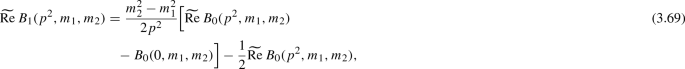
Note that \({\widetilde{{\mathrm {Re}}}}\, \varSigma _\mathrm {T}^{AZ}(0)= \varSigma _\mathrm {T}^{AZ}(0)\) since \(\varSigma _\mathrm {T}^{AZ}(0)\) is free from absorptive parts.
Here all SU(3) generators as well as electromagnetic charges should be understood in terms of incoming charge flow.
Due to our recoil conventions for (off-shell) photon emitters in (3.100), \({\hat{\gamma }}^{\mathrm {QED}}_{\gamma }\) contributions are only relevant for massive initial-state spectators.
A version of SCons (“scons-local”) is shipped with OpenLoops, but a system-wide installation may be used as well.
An installation routine to move the library to a different location is currently not available.
The collection all.coll makes it possible to download the full set of available processes libraries at once. However, due to the large overall number of processes and the presence of several complex processes, this is requires a very large amount of disk space and very long CPU time for compilation. Thus all.coll should not be used for standard applications.
In general, base code and process code can be combined in a rather flexible way, but care must be taken that they remain mutually consistent. The API compatibility between base code and process code is typically guaranteed across many sub-versions, both in the forward and backward directions. To this end, all mutually consistent versions are labelled with the same (internal) API version number, and OpenLoops accepts to use only combinations of process code and base code that belong to the same API version.
The registration procedure through the BLHA is explained in Appendix B.1.
This corresponds to the normalisation convention used by the Collier [19] library.
The values of \(\varDelta _2\), \(\varDelta _{\mathrm {IR},1}\) and \(\varDelta _{\mathrm {UV},1}\) are controlled internally by OpenLoops. For validation purposes they can be changed using the parameters pole_IR2, pole_IR1 and pole_UV1, respectively. However such modifications may jeopardise the calculation of UV and IR divergent quantities.
As usual, the corresponding SU(3)\(\times \)U(1) quantum numbers should be understood in terms of incoming charge flow, in such a way that \(\sum _k T^a_k | \mathcal {M}\big \rangle =\sum _k Q_k | \mathcal {M}\big \rangle =0\).
Explicit expression for \(k_\perp ^{\mu }\) in the dipole subtraction formalism are for example listed in Tab. 1 of [73] for all relevant splittings.
OpenLoops automatically amputates possible non-orthogonal parts of \(k_\perp \) by projecting \(k_\perp ^\mu \) onto \({\varepsilon }^\mu _{\pm }(p_j)\).
Note that (4.40) is computed in the trace basis excluding off-diagonal \(\mathcal {K}_{ij}\) terms but including any other sub-leading-colour contributions.
This estimate is based on the analytic form of all presently known spurious singularities. So far it was found to be quite reliable. However, it may have to be improved if new types of instabilities are encountered.
In the tail of the CutTools curve (not shown) numerical instabilities can reach and largely exceed \(\mathcal {O}(10^{10})\).
For performance reasons, by default the (negative) IR poles of the \({{\mathbf {I}}}\)-operator, Eq. (3.98), are returned as IR poles in m2l1. The true poles of the virtual amplitudes can be obtained by setting the parameter \(\texttt {truepoles=1}\). Alternatively setting \(\texttt {truepoles=2}\) sums the virtual amplitude including its true poles and the \({\mathbf {I}}\)-operator including its finite part and poles, which allows for easy pole cancellation checks. See more details in Sect. 4.3.
For performance reasons, by default the (negative) IR poles of the \({\mathbf {I}}\)-operator and UV counterterm are returned as poles in m2l1bare. The true poles of the bare virtual amplitudes can be obtained by setting the parameter \(\texttt {truepoles=1}\).


References
R. Britto, F. Cachazo, B. Feng, Generalized unitarity and one-loop amplitudes in \(\text{ N }=4\) super-Yang–Mills. Nucl. Phys. B 725, 275–305 (2005). https://doi.org/10.1016/j.nuclphysb.2005.07.014. arXiv:hep-th/0412103
F. del Aguila, R. Pittau, Recursive numerical calculus of one-loop tensor integrals. JHEP 07, 017 (2004). https://doi.org/10.1088/1126-6708/2004/07/017. arXiv:hep-ph/0404120
Z. Bern, L.J. Dixon, D.A. Kosower, Bootstrapping multi-parton loop amplitudes in QCD. Phys. Rev. D 73, 065013 (2006). https://doi.org/10.1103/PhysRevD.73.065013. arXiv:hep-ph/0507005
A. Denner, S. Dittmaier, Reduction schemes for one-loop tensor integrals. Nucl. Phys. B 734, 62–115 (2006). https://doi.org/10.1016/j.nuclphysb.2005.11.007. arXiv:hep-ph/0509141
G. Ossola, C.G. Papadopoulos, R. Pittau, Reducing full one-loop amplitudes to scalar integrals at the integrand level. Nucl. Phys. B 763, 147–169 (2007). https://doi.org/10.1016/j.nuclphysb.2006.11.012. arXiv:hep-ph/0609007
D. Forde, Direct extraction of one-loop integral coefficients. Phys. Rev. D 75, 125019 (2007). https://doi.org/10.1103/PhysRevD.75.125019. arXiv:0704.1835
W.T. Giele, Z. Kunszt, K. Melnikov, Full one-loop amplitudes from tree amplitudes. JHEP 04, 049 (2008). https://doi.org/10.1088/1126-6708/2008/04/049. arXiv:0801.2237
A. van Hameren, Multi-gluon one-loop amplitudes using tensor integrals. JHEP 07, 088 (2009). https://doi.org/10.1088/1126-6708/2009/07/088. arXiv:0905.1005
F. Cascioli, P. Maierhöfer, S. Pozzorini, Scattering amplitudes with open loops. Phys. Rev. Lett. 108, 111601 (2012). https://doi.org/10.1103/PhysRevLett. arXiv:1111.5206
G. Ossola, C.G. Papadopoulos, R. Pittau, CutTools: a program implementing the OPP reduction method to compute one-loop amplitudes. JHEP 03, 042 (2008). https://doi.org/10.1088/1126-6708/2008/03/042. arXiv:0711.3596
C.F. Berger, Z. Bern, L.J. Dixon, F.Febres Cordero, D. Forde, H. Ita, D.A. Kosower, D. Maitre, An automated implementation of on-shell methods for one-loop amplitudes. Phys. Rev. D 78, 036003 (2008). https://doi.org/10.1103/PhysRevD.78.036003. arXiv:0803.4180
A. van Hameren, C.G. Papadopoulos, R. Pittau, Automated one-loop calculations: a proof of concept. JHEP 09, 106 (2009). https://doi.org/10.1088/1126-6708/2009/09/106. arXiv:0903.4665
V. Hirschi, R. Frederix, S. Frixione, M.V. Garzelli, F. Maltoni, R. Pittau, Automation of one-loop QCD corrections. JHEP 05, 044 (2011). https://doi.org/10.1007/JHEP05(2011). arXiv:1103.0621
P. Mastrolia, G. Ossola, T. Reiter, F. Tramontano, Scattering amplitudes from unitarity-based reduction algorithm at the integrand-level. JHEP 08, 080 (2010). https://doi.org/10.1007/JHEP08(2010). arXiv:1006.0710
S. Badger, B. Biedermann, P. Uwer, V. Yundin, Numerical evaluation of virtual corrections to multi-jet production in massless QCD. Comput. Phys. Commun. 184, 1981–1998 (2013). https://doi.org/10.1016/j.cpc.2013.03.018. arXiv:1209.0100
F. Cascioli, J. M. Lindert, P. Maierhöfer, S. Pozzorini, The OpenLoops one-loop generator, Publicly. http://openloops.hepforge.org
G. Cullen et al., \(\text{ G }O\text{ S }AM\)-2.0: a tool for automated one-loop calculations within the Standard Model and beyond. Eur. Phys. J. C 74(8), 3001 (2014). https://doi.org/10.1140/epjc/s10052-014-3001-5. arXiv:1404.7096
T. Peraro, Ninja: automated integrand reduction via laurent expansion for one-loop amplitudes. Comput. Phys. Commun. 185, 2771–2797 (2014). https://doi.org/10.1016/j.cpc.2014.06.017. arXiv:1403.1229
A. Denner, S. Dittmaier, L. Hofer, Collier: a fortran-based complex one-loop library in extended regularizations. Comput. Phys. Commun. 212, 220–238 (2017). https://doi.org/10.1016/j.cpc.2016.10.013. arXiv:1604.06792
S. Actis, A. Denner, L. Hofer, J.-N. Lang, A. Scharf, S. Uccirati, RECOLA: recursive computation of one-loop amplitudes. Comput. Phys. Commun. 214, 140–173 (2017). https://doi.org/10.1016/j.cpc.2017.01.004. arXiv:1605.01090
Z. Bern, L.J. Dixon, F.Febres Cordero, S. Höche, H. Ita, D.A. Kosower, D. Mal̂tre, K.J. Ozeren, Next-to-leading order \(W + 5\)-jet production at the LHC. Phys. Rev. D 88(1), 014025 (2013). https://doi.org/10.1103/PhysRevD.88.014025. arXiv:1304.1253
S. Badger, B. Biedermann, P. Uwer, V. Yundin, Next-to-leading order QCD corrections to five jet production at the LHC. Phys. Rev. D 89(3), 034019 (2014). https://doi.org/10.1103/PhysRevD.89.034019. arXiv:1309.6585
G. Bevilacqua, H.B. Hartanto, M. Kraus, M. Worek, Top quark pair production in association with a jet with next-to-leading-order QCD off-shell effects at the large hadron collider. Phys. Rev. Lett. 116(5), 052003 (2016). https://doi.org/10.1103/PhysRevLett.116.052003. arXiv:1509.09242
S. Höche, P. Maierhöfer, N. Moretti, S. Pozzorini, F. Siegert, Next-to-leading order QCD predictions for top-quark pair production with up to three jets. Eur. Phys. J. C 77(3), 145 (2017). https://doi.org/10.1140/epjc/s10052-017-4715-y. arXiv:1607.06934
A. Denner, J.-N. Lang, M. Pellen, S. Uccirati, Higgs production in association with off-shell top-antitop pairs at NLO EW and QCD at the LHC. JHEP 02, 053 (2017). https://doi.org/10.1007/JHEP02(2017). arXiv:1612.07138
T. Gleisberg, S. Hoeche, F. Krauss, M. Schönherr, S. Schumann, F. Siegert, J. Winter, Event generation with SHERPA 1.1. JHEP 02, 007 (2009). https://doi.org/10.1088/1126-6708/2009/02/007. arXiv:0811.4622
S. Alioli, P. Nason, C. Oleari, E. Re, A general framework for implementing NLO calculations in shower Monte Carlo programs: the POWHEG BOX. JHEP 06, 043 (2010). https://doi.org/10.1007/JHEP06(2010). arXiv:1002.2581
G. Bevilacqua, M. Czakon, M.V. Garzelli, A. van Hameren, A. Kardos, C.G. Papadopoulos, R. Pittau, M. Worek, HELAC-NLO. Comput. Phys. Commun. 184, 986–997 (2013). https://doi.org/10.1016/j.cpc.2012.10.033. arXiv:1110.1499
J. Alwall, R. Frederix, S. Frixione, V. Hirschi, F. Maltoni, O. Mattelaer, H.S. Shao, T. Stelzer, P. Torrielli, M. Zaro, The automated computation of tree-level and next-to-leading order differential cross sections, and their matching to parton shower simulations. JHEP 07, 079 (2014). https://doi.org/10.1007/JHEP07(2014). arXiv:1405.0301
T. Sjöstrand, S. Ask, J.R. Christiansen, R. Corke, N. Desai, P. Ilten, S. Mrenna, S. Prestel, C.O. Rasmussen, P.Z. Skands, An Introduction to PYTHIA 8.2. Comput. Phys. Commun. 191, 159–177 (2015). https://doi.org/10.1016/j.cpc.2015.01.024. arXiv:1410.3012
C. Weiss, B.Chokoufe Nejad, W. Kilian, J. Reuter, Automated NLO QCD Corrections with WHIZARD. PoS EPS-HEP 2015, 466 (2015). arXiv:1510.02666
J. Bellm et al., Herwig 7.0/Herwig++ 3.0 release note. Eur. Phys. J. C 76(4), 196 (2016). https://doi.org/10.1140/epjc/s10052-016-4018-8. arXiv:1512.01178
F. Buccioni, S. Pozzorini, M. Zoller, On-the-fly reduction of open loops. Eur. Phys. J. C 78(1), 70 (2018). https://doi.org/10.1140/epjc/s10052-018-5562-1. arXiv:1710.11452
A. Denner, S. Dittmaier, Reduction of one-loop tensor 5-point integrals. Nucl. Phys. B 658, 175–202 (2003). https://doi.org/10.1016/S0550-3213(03)00184-6
S. Kallweit, J.M. Lindert, P. Maierhöfer, S. Pozzorini, M. Schönherr, NLO electroweak automation and precise predictions for W+multijet production at the LHC. JHEP 04, 012 (2015). https://doi.org/10.1007/JHEP04(2015). arXiv:1412.5157
S. Kallweit, J.M. Lindert, S. Pozzorini, M. Schönherr, NLO QCD+EW predictions for \(2\ell 2\nu \) diboson signatures at the LHC. JHEP 11, 120 (2017). https://doi.org/10.1007/JHEP11(2017). arXiv:1705.00598
A. Denner, Techniques for calculation of electroweak radiative corrections at the one loop level and results for W physics at LEP-200. Fortsch. Phys. 41, 307–420 (1993). https://doi.org/10.1002/prop.2190410402. arXiv:0709.1075
A. Denner, S. Dittmaier, M. Roth, L. H. Wieders, Electroweak corrections to charged-current e+ e- —> 4 fermion processes: technical details and further results, Nucl. Phys. B724, 247–294 (2005). [Erratum: Nucl. Phys.B854,504(2012)]. arXiv:hep-ph/0505042, https://doi.org/10.1016/j.nuclphysb.2011.09.001, https://doi.org/10.1016/j.nuclphysb.2005.06.033
S. Catani, M. H. Seymour, A general algorithm for calculating jet cross-sections in NLO QCD, Nucl. Phys. B485, 291–419 (1997) [Erratum: Nucl. Phys.B510,503(1998)]. arXiv:hep-ph/9605323, https://doi.org/10.1016/S0550-3213(96)00589-5, https://doi.org/10.1016/S0550-3213(98)81022-5
S. Catani, S. Dittmaier, M.H. Seymour, Z. Trocsanyi, The dipole formalism for next-to-leading order QCD calculations with massive partons. Nucl. Phys. B 627, 189–265 (2002). https://doi.org/10.1016/S0550-3213(02)00098-6. arXiv:hep-ph/0201036
S. Dittmaier, A general approach to photon radiation off fermions. Nucl. Phys. B 565, 69–122 (2000). https://doi.org/10.1016/S0550-3213(99)00563-5. arXiv:hep-ph/9904440
S. Dittmaier, A. Kabelschacht, T. Kasprzik, Polarized QED splittings of massive fermions and dipole subtraction for non-collinear-safe observables. Nucl. Phys. B 800, 146–189 (2008). https://doi.org/10.1016/j.nuclphysb.2008.03.010. arXiv:0802.1405
T. Gehrmann, N. Greiner, Photon radiation with maddipole. JHEP 12, 050 (2010). https://doi.org/10.1007/JHEP12(2010). arXiv:1011.0321
M. Schönherr, An automated subtraction of NLO EW infrared divergences. Eur. Phys. J. C 78(2), 119 (2018). https://doi.org/10.1140/epjc/s10052-018-5600-z. arXiv:1712.07975
T. Binoth, et al., A Proposal for a standard interface between Monte Carlo tools and one-loop programs, Comput. Phys. Commun. 181, 1612–1622 (2010). [,1(2010)]. arXiv:1001.1307, https://doi.org/10.1016/j.cpc.2010.05.016
S. Alioli et al., Update of the Binoth Les Houches Accord for a standard interface between Monte Carlo tools and one-loop programs. Comput. Phys. Commun. 185, 560–571 (2014). https://doi.org/10.1016/j.cpc.2013.10.020. arXiv:1308.3462
E. Bothmann, et al., Event generation with SHERPA 2.2. arXiv:1905.09127
S. Alioli, C.W. Bauer, C.J. Berggren, A. Hornig, F.J. Tackmann, C.K. Vermilion, J.R. Walsh, S. Zuberi, Combining higher-order resummation with multiple NLO calculations and parton showers in GENEVA. JHEP 09, 120 (2013). https://doi.org/10.1007/JHEP09(2013). arXiv:1211.7049
W. Kilian, T. Ohl, J. Reuter, WHIZARD: simulating multi-particle processes at LHC and ILC. Eur. Phys. J. C 71, 1742 (2011). https://doi.org/10.1140/epjc/s10052-011-1742-y. arXiv:0708.4233
M. Grazzini, S. Kallweit, M. Wiesemann, Fully differential NNLO computations with MATRIX. Eur. Phys. J. C 78(7), 537 (2018). https://doi.org/10.1140/epjc/s10052-018-5771-7. arXiv:1711.06631
S. Kallweit, J.M. Lindert, P. Maierhöfer, S. Pozzorini, M. Schönherr, NLO QCD+EW predictions for V + jets including off-shell vector-boson decays and multijet merging. JHEP 04, 021 (2016). https://doi.org/10.1007/JHEP04(2016). arXiv:1511.08692
C. Gütschow, J.M. Lindert, M. Schönherr, Multi-jet merged top-pair production including electroweak corrections. Eur. Phys. J. C 78(4), 317 (2018). https://doi.org/10.1140/epjc/s10052-018-5804-2. arXiv:1803.00950
M. Grazzini, S. Kallweit, J. M. Lindert, S. Pozzorini, M. Wiesemann, Giant QCD K-factors and large EW corrections: NNLO QCD+EW for vector-boson pair production (in preparation)
T. Hahn, Generating Feynman diagrams and amplitudes with FeynArts 3. Comput. Phys. Commun. 140, 418–431 (2001). https://doi.org/10.1016/S0010-4655(01)00290-9. arXiv:hep-ph/0012260
J.A.M. Vermaseren, Axodraw. Comput. Phys. Commun. 83, 45–58 (1994)
G. Ossola, C.G. Papadopoulos, R. Pittau, On the rational terms of the one-loop amplitudes. JHEP 05, 004 (2008). https://doi.org/10.1088/1126-6708/2008/05/004. arXiv:0802.1876
P. Draggiotis, M.V. Garzelli, C.G. Papadopoulos, R. Pittau, Feynman rules for the rational part of the QCD 1-loop amplitudes. JHEP 04, 072 (2009). https://doi.org/10.1088/1126-6708/2009/04/072. arXiv:0903.0356
M. V. Garzelli, I. Malamos, R. Pittau, Feynman rules for the rational part of the Electroweak 1-loop amplitudes. JHEP 01, 040 (2010), [Erratum: JHEP10,097(2010)]. arXiv:0910.3130, https://doi.org/10.1007/JHEP10(2010)097, https://doi.org/10.1007/JHEP01(2010)040
M.V. Garzelli, I. Malamos, R. Pittau, Feynman rules for the rational part of the electroweak 1-loop amplitudes in the \(R_xi\) gauge and in the unitary gauge. JHEP 01, 029 (2011). https://doi.org/10.1007/JHEP01(2011). arXiv:1009.4302
M.V. Garzelli, I. Malamos, R2SM: a package for the analytic computation of the \(R_2\) rational terms in the standard model of the electroweak interactions. Eur. Phys. J. C 71, 1605 (2011). https://doi.org/10.1140/epjc/s10052-011-1605-6. arXiv:1010.1248
H.-S. Shao, Y.-J. Zhang, K.-T. Chao, Feynman rules for the rational part of the standard model one-loop amplitudes in the ’t Hooft-Veltman \(\gamma _5\) scheme. JHEP 09, 048 (2011). https://doi.org/10.1007/JHEP09(2011). arXiv:1106.5030
R. Pittau, Primary Feynman rules to calculate the epsilon-dimensional integrand of any 1-loop amplitude. JHEP 02, 029 (2012). https://doi.org/10.1007/JHEP02(2012). arXiv:1111.4965
B. Page, R. Pittau, \(R_{2}\) vertices for the effective ggH theory. JHEP 09, 078 (2013). https://doi.org/10.1007/JHEP09(2013). arXiv:1307.6142
A. Denner, S. Dittmaier, Scalar one-loop 4-point integrals. Nucl. Phys. B 844, 199–242 (2011). https://doi.org/10.1016/j.nuclphysb.2010.11.002
A. van Hameren, OneLOop: For the evaluation of one-loop scalar functions. Comput. Phys. Commun. 182, 2427–2438 (2011). https://doi.org/10.1016/j.cpc.2011.06.011. arXiv:1007.4716
F. Buccioni, J.-N. Lang, S. Pozzorini, H. Zhang, M. Zoller, Numerical stability of the on-the-fly method in OpenLoops 2 (in preparation)
R. Frederix, S. Frixione, V. Hirschi, D. Pagani, H.S. Shao, M. Zaro, The automation of next-to-leading order electroweak calculations. JHEP 07, 185 (2018). https://doi.org/10.1007/JHEP07(2018). arXiv:1804.10017
A. Sirlin, Radiative corrections in the SU(2)-L x U(1) theory: a simple renormalization framework. Phys. Rev. D 22, 971–981 (1980). https://doi.org/10.1103/PhysRevD.22.971
M. Tanabashi et al., Review of particle physics. Phys. Rev. D 98(3), 030001 (2018). https://doi.org/10.1103/PhysRevD.98.030001
J. R. Andersen, et al., Les Houches 2013: physics at TeV colliders: standard model working Group Report arXiv:1405.1067
M. Spira, A. Djouadi, D. Graudenz, P.M. Zerwas, Higgs boson production at the LHC. Nucl. Phys. B 453, 17–82 (1995). https://doi.org/10.1016/0550-3213(95)00379-7. arXiv:hep-ph/9504378
S. Dawson, S. Dittmaier, M. Spira, Neutral Higgs boson pair production at hadron colliders: QCD corrections. Phys. Rev. D 58, 115012 (1998). https://doi.org/10.1103/PhysRevD.58.115012. arXiv:hep-ph/9805244
T. Gleisberg, F. Krauss, Automating dipole subtraction for QCD NLO calculations. Eur. Phys. J. C 53, 501–523 (2008). https://doi.org/10.1140/epjc/s10052-007-0495-0. arXiv:0709.2881
S. Frixione, Z. Kunszt, A. Signer, Three jet cross-sections to next-to-leading order. Nucl. Phys. B 467, 399–442 (1996). https://doi.org/10.1016/0550-3213(96)00110-1. arXiv:hep-ph/9512328
A. Kanaki, C.G. Papadopoulos, HELAC: a package to compute electroweak helicity amplitudes. Comput. Phys. Commun. 132, 306–315 (2000). https://doi.org/10.1016/S0010-4655(00)00151-X. arXiv:hep-ph/0002082
F. Maltoni, K. Paul, T. Stelzer, S. Willenbrock, Color flow decomposition of QCD amplitudes. Phys. Rev. D 67, 014026 (2003). https://doi.org/10.1103/PhysRevD.67.014026. arXiv:hep-ph/0209271
R. Kleiss, W.J. Stirling, S.D. Ellis, A new Monte Carlo treatment of multiparticle phase space at high-energies. Comput. Phys. Commun. 40, 359 (1986). https://doi.org/10.1016/0010-4655(86)90119-0
T. Ježo, J.M. Lindert, P. Nason, C. Oleari, S. Pozzorini, An NLO+PS generator for \(t\bar{t}\) and \(Wt\) production and decay including non-resonant and interference effects. Eur. Phys. J. C 76(12), 691 (2016). https://doi.org/10.1140/epjc/s10052-016-4538-2. arXiv:1607.04538
Acknowledgements
We are thankful to Andreas van Hameren for supporting OneLOop, and to Ansgar Denner and Stefan Dittmaier for supporting Collier . We are indebted to Stefan Kallweit for numerous bug reports and pre-release tests. Also we would like to thank the Sherpa and Matrix collaborations for continuous collaboration and discussions. We thank the ATLAS and CMS Monte Carlo groups for valuable feedback. J.M.L. would like to thank the Theoretical Particle Physics group at Sussex University for the hospitality during the completion of this work. F.B., J.-N.L., S.P., H.Z., M.Z. acknowledge support from the Swiss National Science Foundation (SNF) under contract BSCGI0-157722. M.Z. acknowledges support by the Swiss National Science Foundation (Ambizione grant PZ00P2-179877).
Author information
Authors and Affiliations
Corresponding author
Appendices
Appendix A: Native Fortran and C/C++ interfaces
OpenLoops can easily be integrated into Monte Carlo tools via its native interfaces in Fortran and C or via the BLHA interface [45, 46]. The C interface can of course be used from  as well. We recommend to use the native interface, because it is easier to use, provides more functionality and does not require exchanging files between the tools. In this Appendix we present the various functionalities of the native OpenLoops interface. In doing so we will always refer to the names of the relevant Fortran interface functions. The corresponding C functions are named in the same way with an extra ol_ prefix. In Appendix A.1 we detail necessary modules to be loaded (Fortran) and required header files (C/
 ) together with conventions for the format of phase-space points for the evaluation of scattering amplitudes. In Appendix A.2 the setting of parameters is discussed and in Appendix A.3 the registration of processes. In Appendix A.4-Appendix A.8 we detail the various interfaces for the evaluation of squared scattering amplitudes, amplitude correlators and amplitude colour vectors. Finally, in Appendix A.9 we give a basic example for the usage of the native OpenLoops interface in Fortran and C.
The implementation of the BLHA interface and the usage of OpenLoops together with Sherpa and Powheg-Box are discussed in Appendix B.
1.1 Appendix A.1: Generalities
Fortran interface In order to use the native Fortran interface, the module openloops must be included with

The module files are located in the directory lib_src/openloops/mod, which should be added to the include path of the Fortran compiler.
Floating point numbers used in the interface are in double precision, denoted here by the kind type dp which can be obtained as follows:

Phase space points p_ex are passed as two-dimensional arrays declared as

Here and in the following N stands for the number of incoming plus outgoing external particles of the considered process. External particles are numbered from 1 to N and are interpreted as incoming or outgoing according to the process registration. See (4.1) and below. The entries p_ex(i,K) correspond to the energy (i=0) and the three physical momentum components (i=1, 2, 3) of particle K in GeV units.
C interface The C interface is declared in the the header file include/openloops.h and can be included in C and  code. Phase space points pp are passed as one-dimensional arrays with 5N components, where every fifth component is the mass of the corresponding external particle (BLHA convention), i.e. phase-space points in the C interface are declared as

The fifth component is currently not used within OpenLoops.
1.2 Appendix A.2: Parameter setting
In order to set the OpenLoops parameter with name key to the value val, call

where TYPE is integer, real(dp) or character(*) depending on the type of the parameter. It is possible to set parameters of integer or real(dp) type by passing the value in string representation. The error code err will be zero on success.
In C, the function to set a parameter depends on the parameter type:

ol_setparameter_string() may be used to set integer or double precision values given in string representation. The functions do not return an error code, but it may be retrieved by calling

right after setting a parameter. A return value of 0 means that no error occured in the preceeding call.
With the default settings, the program will terminate in case of an error. This can be changed by adjusting the warning level using the function

where level=0 means that errors are silently ignored, level=1 means that a warning message is printed, and level=2 (default) means that the program will be terminated on error.
The current value of a parameter can be retrieved by calling

Retrieving parameter values is only supported for integer and double precision parameter types.
A list of all parameters can be written to a file

For an empty file name, i.e. file=””, the output is written to stdout.
1.3 Appendix A.3: Process registration
As detailed in Sect. 4.2 before evaluation a process has to be registered. This proceeds via

which takes the process as a string in the format “\({\mathrm{PID}}_{i,1} \dots {\mathrm{PID}}_{i,n}\) \(\texttt {->}\, {\mathrm{PID}}_{f,1} \dots {\mathrm{PID}}_{f,m}\)” for a \(n\rightarrow m\) process, where the various particle identifiers (PID) are enetered in either of the two particle labelling schemes specified in Table 6. Alternatively, \(2\rightarrow N-2\) processes can be registered by entering process as an array of integers of length N, where the first two entries are interpreted as initial-state particles. Additionally the amplitude type amptype has to be passed as argument. For the possible values of amptype see Table 4. The function register_process returns the process ID to be used in the routines to evaluate matrix elements, where it is denoted as id.
In the corresponding C interface for process registration

the process can only be passed as a string. Again, the process ID is returned.
When all processes are registered the following function must be called before calculating matrix elements.

When the calculation is finished, i.e. no more matrix elements will be calculated, the following function should be called.

While these calls are not strictly necessary, if log files are used, the files may not be updated at the end of the run and therefore lack information. Additionally, dynamically allocated memory will be deallocated upon the finish call.
1.4 Appendix A.4: Scattering amplitudes
The following interface functions evaluate the scattering probability densities (2.1)–(2.3) and their building blocks described in Sect. 4.3. The required inputs are the integer identifier id of the desired process and the phase-space point p_ex (Fortran) / pp ( ), as defined in Appendix A.1.
Tree-level amplitudes
The function evaluate_tree evaluates the tree–tree probability density (2.1) returning as output \(\texttt {m2l0}=\mathcal {W}_{00}\).

One-loop NLO amplitudes The function evaluate_loop evaluates the UV renormalised Born–one-loop interference (2.2) returning \(\texttt {m2l0}=\mathcal {W}_{00}\) and \(\texttt {m2l1}=\{\mathcal {W}_{01}^{(0)}, \mathcal {W}_{01}^{(1)},\mathcal {W}_{01}^{(2)}\}\) as output. The three values in m2l1 represent the finite part, and the coefficients of the IR single and double polesFootnote 39 of the Born–one-loop interference, as defined in Eq. (4.2). Together with the one-loop amplitude an accuracy estimate is returned (depending on the employed stability system) as acc with \(\texttt {acc}=-1\) in case no stability estimate is available. When available, acc quantifies the relative accuracy \(\delta \mathcal {W}_{01}^{(0)}/\mathcal {W}_{01}^{(0)}\), and \(\texttt {acc}=10^{-a}\) corresponds to an estimated accuracy of a decimal digits.

As documented in Sect. 4.3, various technical parameters permit to activate and deactivated the different building blocks of one-loop amplitudes and to change the normalisation convention for UV and IR poles.
Bare d=4 amplitudes The function evaluate_loopbare evaluates the unrenormalised Born–one-loop interference without UV and \(R_2\) counterterm contributions (i.e. with \(d=4\) loop numerator) as defined in (4.4), returning \(\texttt {m2l0}=\mathcal {W}_{00}\), \(\texttt {m2l1bare}=\{\mathcal {W}_{01,4\mathrm {D}}^{(0)},\mathcal {W}_{01,4\mathrm {D}}^{(1)},\mathcal {W}_{01,4\mathrm {D}}^{(2)} \}\) and an accuracy estimate (see above) acc as output. The three values in m2l1bare represent the finite part and the coefficients of the (UV and IR) single and the double poles.Footnote 40

UV counterterms The function evaluate_loopct evaluates the UV counterterm matrix element, as defined in (4.4) returning \(\texttt {m2l0}=\mathcal {W}_{00}\) and \(\texttt {m2ct}=\{\mathcal {W}_{01,\mathrm {CT}}^{(0)},\mathcal {W}_{01,\mathrm {CT}}^{(1)},\mathcal {W}_{01,\mathrm {CT}}^{(2)} \}\) as output. The three values in m2ct represent the finite part and the coefficients of the (UV) single and double poles, where the latter is always zero.

For performance reasons we also provide the function evaluate_ct, which evaluates only the finite part of the UV counterterm, defined in (4.4), returning \(\texttt {m2ct0}=\mathcal {W}_{01,\mathrm {CT}}^{(0)}\) and \(\texttt {m2l0}=\mathcal {W}_{00}\) as output.

\(R_2\)counterterms The function evaluate_r2 evaluates the \(R_2\) counterterm matrix element defined in (4.4), returning \(\texttt {m2r2}=\mathcal {W}_{01,R_2}\) and \(\texttt {m2l0}=\mathcal {W}_{00}\).

Pole residues The function evaluate_poles evaluates the residues of the UV and IR poles of all ingredients to a Born–one-loop interference defined in (4.4) including also the I-operator. As output it returns \(\texttt {m2l0}=\mathcal {W}_{00}\), \(\texttt {m2bare}=\{\mathcal {W}_{01,4\mathrm {D}}^{(1,\mathrm {UV})},\mathcal {W}_{01,4\mathrm {D}}^{(1,\mathrm {IR})},\mathcal {W}_{01,4\mathrm {D}}^{(2,\mathrm {IR})} \}\), \(\texttt {m2ct}=\{\mathcal {W}_{01,\mathrm {CT}}^{(1,\mathrm {UV})},\mathcal {W}_{01,\mathrm {CT}}^{(1,\mathrm {IR})},\mathcal {W}_{01,\mathrm {CT}}^{(2,\mathrm {IR})} \}\), \(\texttt {m2ir}=\{\mathcal {W}_{00, \hbox {I-op}}^{(1,\mathrm {UV})},\mathcal {W}_{00, \hbox {I-op}}^{(1,\mathrm {IR})},\mathcal {W}_{00, \hbox {I-op}}^{(2,\mathrm {IR})} \}\) and \(\texttt {m2sum}=\texttt {m2bare}+\texttt {m2ct}+\texttt {m2ir}\). The three values in m2bare, m2ct, m2ir, m2sum correspond respectively to the residues of the \(1/{\varepsilon }_{\mathrm {UV}}\), \(1/{\varepsilon }_{\mathrm {IR}}\) and \(1/{\varepsilon }_{\mathrm {IR}}^2\) poles. For automated pole cancellation checks the output of this routine can automatically be printed to the screen upon amplitude registration when the parameter \(\texttt {check\_poles}=1\) is set.

Squared one-loop amplitudes The function evaluate_loop2 evaluates the squared one-loop matrix element (2.3) returning \(\texttt {m2l2}=\mathcal {W}_{11}\) and a relative accuracy estimate \(\texttt {acc}=\delta \mathcal {W}_{11}/\mathcal {W}_{11}\) (depending on the stability settings) as output.

1.5 Appendix A.5: \({\mathbf {I}}\)-operator
Tree–tree \({\mathbf {I}}\)-operator insertions The function evaluate_iop evaluates the \({\mathbf {I}}\)-operator insertion into a squared Born amplitude, as defined in (3.97), returning \(\texttt {m2l0}=\mathcal {W}_{00}\) and \(\texttt {m2ir}=\{\mathcal {W}_{00, \hbox {I-op}}^{(0)},\mathcal {W}_{00, \hbox {I-op}}^{(1)},\mathcal {W}_{00, \hbox {I-op}}^{(2)}\}\). The three values in m2ir represent the finite part and the coefficients of the (IR) single and double poles.

Loop-loop \({\mathbf {I}}\)-operator insertions The function evaluate_loop2iop evaluates the \({\mathbf {I}}\)-operator insertion into a squared one-loop amplitude as defined in (3.97), returning \(\texttt {m2l2}=\mathcal {W}_{11}\) and \(\texttt {m2l2ir}=\{\mathcal {W}_{11,\hbox {I-op}}^{(0)},\mathcal {W}_{11,\hbox {I-op}}^{(1)},\mathcal {W}_{11,\hbox {I-op}}^{(2)}\}\). The three values in m2l2ir represent the finite part and the coefficients of the (IR) single and double poles in a Laurent series similar to (4.2).

1.6 Appendix A.6: Colour and charge correlators
Tree–tree colour correlators The function evaluate_ccmatrix returns the full matrix of colour-correlated squared tree amplitudes as defined in (4.7), returning \(\texttt {m2l0}=\mathcal {W}_{00}\) and a two-dimensional array \(\texttt {m2cc}\) \(\texttt {matrix(i,j)}={\mathcal {C}}^{(p,q|ij)}_{00,{\scriptscriptstyle \mathrm {LO}}\, {\scriptscriptstyle {\mathrm {QCD}}}} \) (Fortran) or a one-dimensional array \(\texttt {m2ccmatrix}[(i-1)*\hbox {N}+\hbox {j}-1]={\mathcal {C}}^{(p,q|ij)}_{00,{\scriptscriptstyle \mathrm {LO}}\, {\scriptscriptstyle {\mathrm {QCD}}}} \) (C). m2ewcc is reserved for the associated charge-correlated born amplitude, but is currently not in use.

Alternatively the function evaluate_cc evaluates only the \(N(N-1)/2\) independent colour-correlated squared tree amplitudes (4.7) in the BLHA convention, returning \(\texttt {m2l0}=\mathcal {W}_{00}\) and \(\texttt {m2cc(i+(j-1)(j-2)/2)}={\mathcal {C}}^{(p,q|ij)}_{00,{\scriptscriptstyle \mathrm {LO}}\, {\scriptscriptstyle {\mathrm {QCD}}}} \) (Fortran) rsp. \(\texttt {m2cc[i+(j-1)(j-2)/2-1]} ={\mathcal {C}}^{(p,q|ij)}_{00,{\scriptscriptstyle \mathrm {LO}}\, {\scriptscriptstyle {\mathrm {QCD}}}}\) (C) with \(1 \le i < j \le N\).

Tree–tree charge correlators The function evaluate_ccewmatrix returns the full matrix of charge-correlated squared tree amplitudes, as defined in (4.8), returning \(\texttt {m2l0}=\mathcal {W}_{00}\) and a two-dimensional array \(\texttt {m2ccewmatrix}\) \(\texttt {(i,j)}={\mathcal {C}}^{(p,q|ij)}_{00,{\scriptscriptstyle \mathrm {LO}}\, {\scriptscriptstyle \mathrm {QED}}} \) (Fortran) or a one-dimensional array \(\texttt {m2ccewmatrix}[(i-1)*\hbox {N}+\hbox {j}-1]={\mathcal {C}}^{(p,q|ij)}_{00,{\scriptscriptstyle \mathrm {LO}}\, {\scriptscriptstyle \mathrm {QED}}} \) (C).

Loop–loop colour correlators The function evaluate_ccmatrix2 returns the full matrix of colour-correlated squared loop amplitudes as defined in (4.7), returning \(\texttt {m2l2}=\mathcal {W}_{11}\) as a two-dimensional array \(\texttt {m2ccmatrix}\) \(\texttt {(i,j)}={\mathcal {C}}^{(p,q|ij)}_{11,{\scriptscriptstyle \mathrm {LO}}\, {\scriptscriptstyle {\mathrm {QCD}}}} \) (Fortran) or as a one-dimensional array \(\texttt {m2ccmatrix}[(i-1)*\hbox {N}+\hbox {j}-1]={\mathcal {C}}^{(p,q|ij)}_{11,{\scriptscriptstyle \mathrm {LO}}\, {\scriptscriptstyle {\mathrm {QCD}}}} \) (C). m2ewcc is reserved for the associated charge-correlated loop-squared amplitude, but is currently not in use.

Similarly as for the colour-correlated Born correlators (see above), the function evaluate_cc2 evaluates only the independent colour-correlated loop-squared amplitudes in the BLHA convention returning \(\texttt {m2l2}=\mathcal {W}_{11}\) and \(\texttt {m2cc(i+(j-1)(j-2)/2)}={\mathcal {C}}^{(p,q|ij)}_{11,{\scriptscriptstyle \mathrm {LO}}\, {\scriptscriptstyle {\mathrm {QCD}}}} \) (Fortran) rsp. \(\texttt {m2cc[i+(j-1)(j-2)/2-1]} ={\mathcal {C}}^{(p,q|ij)}_{11,{\scriptscriptstyle \mathrm {LO}}\, {\scriptscriptstyle {\mathrm {QCD}}}}\) (C) with \(1 \le i < j \le N\).

Loop–Loop charge correlators The function evaluate_ccewmatrix2 computes the full matrix of charge-correlated squared loop amplitudes as defined in (4.8). As output it returns \(\texttt {m2l2}=\mathcal {W}_{11}\) and a two-dimensional array \(\texttt {m2ccewmatrix(i,j)}={\mathcal {C}}^{(p,q|ij)}_{11,{\scriptscriptstyle \mathrm {LO}}\, {\scriptscriptstyle \mathrm {QED}}} \) (Fortran) or a one-dimensional array \(\texttt {m2ccewmatrix}[(i-1)*\hbox {N}+\hbox {j}-1]={\mathcal {C}}^{(p,q|ij)}_{11,{\scriptscriptstyle \mathrm {LO}}\, {\scriptscriptstyle \mathrm {QED}}}\) (C).

Tree–loop colour correlators The function evaluate_loopccmatrix2 returns the full matrix of the finite parts of the colour-correlated Born–loop interferences, as defined in (4.9), returning \(\texttt {m2l0}=\mathcal {W}_{00}\), \(\texttt {m2l1}=\{\mathcal {W}_{01}^{(0)}, \mathcal {W}_{01}^{(1)},\mathcal {W}_{01}^{(2)}\}\) and a two-dimensional array \(\texttt {m2cc}\) \(\texttt {matrix(i,j)}={\mathcal {C}}^{(P,Q|ij)}_{01,{\scriptscriptstyle \mathrm {NLO}}\, {\scriptscriptstyle {\mathrm {QCD}}}} \) (Fortran) or as a one-dimensional array \(\texttt {m2ccmatrix}[(i-1)*\hbox {N}+\hbox {j}-1]={\mathcal {C}}^{(P,Q|ij)}_{01,01, {\scriptscriptstyle \mathrm {NLO}}\, {\scriptscriptstyle {\mathrm {QCD}}}} \) (C). m2ewcc is reserved for the associated charge-correlated Born–loop interference, but is currently not in use.

Similarly as for the colour-correlated Born correlators (see above), the function evaluate_loopcc evaluates only the independent colour-correlated Born–loop interference amplitudes (finite parts only) in the BLHA convention returning \(\texttt {m2l0}=\mathcal {W}_{00}\), \(\texttt {m2l1}=\{\mathcal {W}_{01}^{(0)}, \mathcal {W}_{01}^{(1)},\mathcal {W}_{01}^{(2)}\}\) and \(\texttt {m2cc(i+(j-1)(j-2)/2)}={\mathcal {C}}^{(ij)}_{01, {\scriptscriptstyle \mathrm {NLO}}\, {\scriptscriptstyle {\mathrm {QCD}}}} \) (Fortran) rsp. \(\texttt {m2cc[i+(j-1)(j-2)/2-1]} ={\mathcal {C}}^{(ij)}_{01, {\scriptscriptstyle \mathrm {NLO}}\, {\scriptscriptstyle {\mathrm {QCD}}}}\) (C) with \(1 \le i < j \le N\).

1.7 Appendix A.7: Spin correlators
Tree–tree spin correlators The function evaluate_sc evaluates the colour-spin-correlated squared tree amplitudes (4.18) for a given gluon/photon emitterj and polarisation vector \(\texttt {polvect}=k_\perp \) fulfilling \(k_\perp \cdot p_j=0\). It returns \(\texttt {m2sc(k)}={\mathcal {B}}^{(p,q|jk)}_{LL,{\scriptscriptstyle \mathrm {LO}}}(k_\perp )\) (Fortran), rsp. \(\texttt {m2sc[k-1]}={\mathcal {B}}^{(p,q|jk)}_{LL,{\scriptscriptstyle \mathrm {LO}}}(k_\perp )\) (C) with \(1\le k \le N\).

The function evaluate_sctensor evaluates the colour-spin-correlated squared tree tensor (4.20) for an emitterj returning \(\texttt {m2l0}=\mathcal {W}_{00}\) and as a \(\hbox {N}\times 4\times 4\) array \(\texttt {m2munu(k,mu,nu)}={\mathcal {B}}^{(p,q|jk|\mu \nu )}_{00,{\scriptscriptstyle \mathrm {LO}}}\) (Fortran), rsp. a vector of length (16N), \(\texttt {m2munu[(k-1)*N+(mu-1)*4+}\) \(\texttt {(nu-1)]}={\mathcal {B}}^{(p,q|jk|\mu \nu )}_{00,{\scriptscriptstyle \mathrm {LO}}}\) (C), with \(1\le k \le N\) and \(1 \le \texttt {mu,nu} \le 4\).

The function evaluate_stensor evaluates the spin-correlated squared tree tensor (4.21) (Powheg-Box convention) for an emitterj returning \(\texttt {m2l0}=\mathcal {W}_{00}\) and as a \(4\times 4\) array \(\texttt {m2munu(mu,nu)}={\mathcal {B}}^{(p,q|j|\mu \nu )}_{00,{\scriptscriptstyle \mathrm {LO}}}\) (Fortran), rsp. a vector of length 16, \(\texttt {m2munu[(mu-1)*4+(nu-1)]}={\mathcal {B}}^{(p,q|j|\mu \nu )}_{00,{\scriptscriptstyle \mathrm {LO}}}\) (C), with \(1 \le \texttt {mu,nu} \le 4\).

Loop–loop spin correlators The function evaluate_sc2 evaluates the colour-spin-correlated loop-squared amplitudes (4.18) for a given gluon/photon emitterj and polarisation vector \(\texttt {polvect}=k_\perp \) fulfilling \(k_\perp \cdot p_j=0\). It returns an array of length N, \(\texttt {m2sc(k)}={\mathcal {B}}^{(p,q|jk)}_{11,{\scriptscriptstyle \mathrm {LO}}}(k_\perp )\) (Fortran), rsp. \(\texttt {m2sc[k-1]}={\mathcal {B}}^{(p,q|jk)}_{11,{\scriptscriptstyle \mathrm {LO}}}(k_\perp )\) (C) with \(1 \le k \le N\).

The function evaluate_sctensor2 evaluates the colour-spin-correlated loop-squared tensor (4.21) (Powheg-Box convention) for an emitterj returning \(\texttt {m2l2}=\mathcal {W}_{11}\) and as a \(\hbox {N}\times 4\times 4\) array \(\texttt {m2munu(k,mu,nu)}={\mathcal {B}}^{(p,q|jk|\mu \nu )}_{11,{\scriptscriptstyle \mathrm {LO}}}\) (Fortran), rsp. a vector of length 16N, \(\texttt {m2munu[(k-1)}\) \(\texttt {*N+(mu-1)*4+(nu-1)]}={\mathcal {B}}^{(p,q|jk|\mu \nu )}_{11,{\scriptscriptstyle \mathrm {LO}}}\) (C) with \(1 \le k \le N\) and \(1 \le \texttt {mu,nu} \le 4\).

Alternatively evaluate_stensor2 evaluates the spin-correlated loop-squared tensor (4.20) (Powheg-Box convention) for an emitterj returning \(\texttt {m2l2}=\mathcal {W}_{11}\) and as a \(4\times 4\) array \(\texttt {m2munu(mu,nu)}={\mathcal {B}}^{(p,q|j|\mu \nu )}_{11,{\scriptscriptstyle \mathrm {LO}}}\) (Fortran), rsp. a vector of length 16, \(\texttt {m2munu[(mu-1)*4+(nu-1)]}={\mathcal {B}}^{(p,q|j|\mu \nu )}_{11,{\scriptscriptstyle \mathrm {LO}}}\) (C) with \(1 \le \texttt {mu,nu} \le 4\).

Tree–loop spin correlators The function evaluate_loopsc evaluates the colour-spin-correlated Born–loop interference (finite part) (4.22) for a given gluon/photon emitterj and polarisation vector \(\texttt {polvect}=k_\perp \) fulfilling \(k_\perp \cdot p_j=0\). It returns an array of length N, \(\texttt {m2sc(k)}={\mathcal {B}}^{(P,Q|jk)}_{01,{\scriptscriptstyle \mathrm {NLO}}}(k_\perp )\) (Fortran), rsp. \(\texttt {m2sc[k-1]}={\mathcal {B}}^{(P,Q|jk)}_{01,{\scriptscriptstyle \mathrm {NLO}}}(k_\perp )\) (C) with \(1 \le k \le N\).

The function evaluate_loopsctensor evaluates the colour-spin-correlated Born–loop interference tensor (finite part) (4.23) (Powheg-Box convention) for an emitterj returning as output \(\texttt {m2l0}=\mathcal {W}_{00}\), \(\texttt {m2l1}=\{\mathcal {W}_{01}^{(0)}, \mathcal {W}_{01}^{(1)},\mathcal {W}_{01}^{(2)}\}\) and a \(\hbox {N}\times 4\times 4\) array \(\texttt {m2munu(k,mu,}\) \(\texttt {nu)}={\mathcal {B}}^{(P,Q|jk|\mu \nu )}_{01,{\scriptscriptstyle \mathrm {NLO}}}\) (Fortran), rsp. a vector of length 16N, \(\texttt {m2munu[(k-1)*N+(mu-1)*4+(nu-1)]}={\mathcal {B}}^{(P,Q|j|\mu \nu )}_{11,{\scriptscriptstyle \mathrm {NLO}}}\) (C) with \(1 \le k \le N\) and \(1 \le \texttt {mu,nu} \le 4\).

Alternatively the function evaluate_loopstensor evaluates the spin-correlated Born–loop interference tensor (finite part) (4.24) (Powheg-Box convention) for an emitterj returning \(\texttt {m2l0}=\mathcal {W}_{00}\), \(\texttt {m2l1}=\{\mathcal {W}_{01}^{(0)}, \mathcal {W}_{01}^{(1)},\mathcal {W}_{01}^{(2)}\}\) and a 4\(\times \)4 array \(\texttt {m2munu(mu,nu)}={\mathcal {B}}^{(P,Q|j|\mu \nu )}_{01,{\scriptscriptstyle \mathrm {NLO}}}\) (Fortran), rsp. a vector of length 16, \(\texttt {m2munu[(mu-1)*4}\) \(\texttt {+(nu-1)]}=={\mathcal {B}}^{(P,Q|j|\mu \nu )}_{11,{\scriptscriptstyle \mathrm {NLO}}}\) (C) with \(1 \le \texttt {mu,nu} \le 4\).

1.8 Appendix A.8: Colour basis and tree amplitudes in colour space
Besides calculating squared and colour-summed matrix elements, OpenLoops also provides tree-level amplitudes with full colour information, see Sect. 4.5, required for the matching of parton showers to matrix elements. In the following we describes how to retrieve the colour basis used for a process and the amplitude as a vector in the colour space which is spanned by these basis elements.
Dimension of colour basis and number of helicities The colour basis elements are encoded as integer arrays and must be retrieved once for each process. First one must obtain the following information:
ncolb: the number of basis elements,
colelemsz: the size of the longest basis element,
nheltot: the total number of helicity configurations (including vanishing configurations).
These are returned by the function tree_colbasis_dim for a given process.

Trace basis The function tree_colbasis returns the actual colour basis as a trace basis in a format corresponding to (4.27)–(4.30), encoded as a two-dimensional integer array of the size basis(colelemsz,ncolb) (Fortran) rsp. basis[ncolb][colelemsz] (C). Trailing zeros should be ignored. The two-dimensional array needed indicates if a certain colour interference contributes to the squared amplitude or not. If needed[i][j]=1, the interference of basis elements i and j contributes, if needed[i][j]=0 it does not.

Colour-flow basis Alternatively the function tree_colourflow returns the basis in colour flow representation, as defined in Eq. (4.35). The format of the basis is flowbasis(2,N,ncolb) (Fortran) rsp. flowbasis[ncolb][N][2] (C), defining ncolb colour flows.

Tree amplitudes in colour space Now, the function evaluate_tree_colvect returns the (complex) tree-level amplitude \(\texttt {amp}=\{\mathcal {A}_0^{(i)}(h)\}\), defined in (4.25), as a vector in the colour space spanned by the colour basis elements for each of the nhelnonv non-vanishing helicity configurations, which may be smaller than the total number of helicity configurations nheltot returned by tree_colbasis_dim(). In Fortranamp(:,h) for h=1..nhelnonv is an array of ncolb complex numbers such that the element amp(i,h) corresponds to the colour basis element basis(:,i). In C amp[h] for h=0..nhelnonv-1 is an array of 2*ncolb real numbers such that the elements amp[h][2*i] and amp[h][2*i+1] are the real and imaginary parts of the amplitude which corresponds to the colour basis element basis[i]. Note that colour and helicity average factors and symmetry factors must still be applied when the squared amplitude is built from these results. See (4.32) and (4.39)–(4.40).

Squared tree amplitudes in colour space Finally, the function evaluate_tree_colvect2 evaluates the squared amplitudes for the colour basis elements, i.e. the diagonal elements of the colour interference matrix (4.40), returning a vector of ncolb elements as \(\texttt {m2arr}(i)=\big |\mathcal {A}^{(i)}_{0}\big |^2\) (Fortran), rsp. \(\texttt {m2arr}[i-1]=\big |\mathcal {A}^{(i)}_{0}\big |^2\) (C). This is meant to calculate the probability with which a matched parton shower should start from the corresponding colour flow. Note that the results are only correct to leading colour approximation and may contain (or even be purely) sub-leading colour contributions.

1.9 Appendix A.9: Basic examples
Here we give a basic example, both for Fortran and C, which illustrates the usage of the native OpenLoops interface. In these examples the process \(d\bar{d}\rightarrow Zu\bar{u}\) is registered via order_ew=1, i.e. the leading tree-level order corresponds to \(\mathcal {O}(\alpha _{\mathrm {s}}^2\alpha )\) and the one-loop order corresponds to the \(\mathcal {O}(\alpha _{\mathrm {s}}^3\alpha )\) NLO QCD corrections. Similar examples are shipped with the OpenLoops installation as ./examples/OL_fortran.f90 and ./examples/OL_cpp.cpp respectively.

Appendix B: Other interfaces
OpenLoops has been integrated in a number of Monte Carlo frameworks. In particular OpenLoops can be used in conjunction with Sherpa [26, 47], Munich/Matrix [50],  [32], Powheg-Box [27], Whizard [49] and Geneva [48]. In Appendix B.1 we detail the BLHA interface within OpenLoops, and in Appendix B.2 and Appendix B.3 the usage of OpenLoops within Sherpa and Powheg-Box respectively. Finally in Appendix B.4 we briefly introduce the OpenLoops Python command line tool.
1.1 Appendix B.1: BLHA interface
OpenLoops offers an interface in the Binoth-Les-Houches-Accord in both versions BLHA1 [45] and BLHA2 [46]. In order to use the Fortran BLHA interface, the module openloops_blha must be included with

The module files are located in the directory lib_src/openloops/mod, which should be added to the include path of the Fortran compiler. In a C/ program the openloops.h header has to be included. In the following we list the scope of the BLHA interface within a
  program. Usage within a Fortran program proceeds analogous.
Within a  program an BLHA contract file is read by OpenLoops via

The answer file is either written to the same file or in a file specified in the contract file via

Parameters are either set via the contract file or directly via the procedure

Furthermore a list of the actual parameter settings can be written to a file filename via

At runtime the tree and loop amplitudes for a phase-space point of N external particles with momenta pp, as specified in the BLHA1/BLHA2 standards, are obtained via

Here, id is the ID of the corresponding subprocess (specified in the answer file), muren the renormalisation scale and alphaS the strong coupling constant. The result is written into the array result, where result[3] gives the tree amplitude and result[2] the finite part, result[1] the single pole and result[0] the double pole of the one-loop amplitude \(\mathcal {W}_{01}\).
A corresponding routine of the BLHA2 standard is also implemented:

Here, additionally an accuracy measure of the corresponding amplitude is returned as acc. When not available acc=-1 is returned. For further details see the specification of the BLHA1 [45] and BLHA2 [46] standards. An example illustrating the usage of the BLHA interface with OpenLoops is shipped as ./examples/OL_blha.cpp.
1.2 Appendix B.2: Sherpa
OpenLoops can be used as a plug-in of Sherpa 2.1.0 or later. Within upcoming releases of Sherpa also the EW subtraction [44] will become publicly available. For the installation of Sherpa and the usage of Sherpa+OpenLoops please also refer to the Sherpa documentation available at https://sherpa.hepforge.org.
In order to use OpenLoops together with Sherpa the Sherpa+OpenLoops interface has to be compiled together with Sherpa passing the --enable-openloops option together with the OpenLoops installation path to the Sherpa configure script. The OpenLoops installation path can be modified at runtime by setting (in the Sherpa run card or command line):

In order to run Sherpa in combination with OpenLoops it is sufficient to add to the Sherpa run card the statement

which includes OpenLoops in the list of available matrix element generators, and to set in the processes section of the Sherpa run card the flag

Sherpa will now automatically use the one-loop matrix elements from OpenLoops when for example a parton-shower matched simulation is requested via (in the processes section of the run card)

For details on these modes and many other options we refer to the Sherpa documentation.
An example run card illustrating the use of Sherpa+OpenLoops can be found within the installation of Sherpa in the file

Additional examples of Sherpa+OpenLoops run cards can be found in the Sherpa manual.
In general Sherpa automatically handles all the necessary parameter initialisation of OpenLoops. However, user-defined parameters can be passed from the Sherpa run card (or command line) to OpenLoops via

1.3 Appendix B.3: POWHEG-BOX
Internally the Powheg-Box+OpenLoops framework automatically compiles, loads and manages all required OpenLoops amplitude libraries. The interface provides the subroutines openloops_born, openloops_real, and openloops_virtual with interfaces identical to the corresponding Powheg-Box routines setborn, setreal, and setvirtual including colour- and spin-correlated tree-level amplitudes in the format required by the Powheg-Box. Additionally, the interface provides the routines openloops_init, openloops_borncolour and openloops_realcolour. The former synchronises all parameters between OpenLoops and the Powheg-Box and should be called at the end of the init processes subroutine of the Powheg-Box. The latter two provide colour information required for parton-shower matching, i.e. they return a colour-flow of the squared Born and real matrix elements in leading-colour approximation, on a probabilistic basis. Further details are given in Appendix A.3 of [78].
1.4 Appendix B.4: Python
OpenLoops provides a Python module openloops.py in the directory pyol/tools that wraps a subset of the functionality of the native interface. Its main application is to provide a simple command line tool to evaluate matrix elements. The documentation of the command line tool can be obtained via

For example the following command evaluates the tree and one-loop amplitudes for \(n=10\) random phase-space points with a center-of-mass energy \(\sqrt{\hat{s}}=500\) GeV for the process \(u \bar{u} \rightarrow Z g g\) using \(M_Z=91\) GeV and prints the result to the screen:

The random phase-space points are generated with Rambo [77].
Appendix C: List of input parameters
In Tables 9, 10, 11 we list all input parameters and switches available in OpenLoops. Within the general purpose Monte Carlo frameworks (e.g. Sherpa, Powheg-Box and  ) these parameters are synchronised automatically.
In Table 9 input parameters relevant for the process registration are listed, in Table 10 model input parameters are listed and in Table 9 input parameters relevant for the stability system are summarised.
Rights and permissions
Open Access This article is distributed under the terms of the Creative Commons Attribution 4.0 International License (http://creativecommons.org/licenses/by/4.0/), which permits unrestricted use, distribution, and reproduction in any medium, provided you give appropriate credit to the original author(s) and the source, provide a link to the Creative Commons license, and indicate if changes were made.
Funded by SCOAP3
About this article

Cite this article
Buccioni, F., Lang, JN., Lindert, J.M. et al. OpenLoops 2. Eur. Phys. J. C 79, 866 (2019). https://doi.org/10.1140/epjc/s10052-019-7306-2
Received:
Accepted:
Published:
DOI: https://doi.org/10.1140/epjc/s10052-019-7306-2