


Summary
Forecasts of future dangerousness are often used to inform the sentencing decisions of convicted offenders. For individuals who are sentenced to probation or paroled to community supervision, such forecasts affect the conditions under which they are to be supervised. The statistical criterion for these forecasts is commonly called recidivism, which is defined as a charge or conviction for any new offence, no matter how minor. Only rarely do such forecasts make distinctions on the basis of the seriousness of offences. Yet seriousness may be central to public concerns, and judges are increasingly required by law and sentencing guidelines to make assessments of seriousness. At the very least, information about seriousness is essential for allocating scarce resources for community supervision of convicted offenders. The paper focuses only on murderous conduct by individuals on probation or parole. Using data on a population of over 60000 cases from Philadelphia’s Adult Probation and Parole Department, we forecast whether each offender will be charged with a homicide or attempted homicide within 2 years of beginning community supervision. We use a statistical learning approach that makes no assumptions about how predictors are related to the outcome. We also build in the costs of false negative and false positive charges and use half of the data to build the forecasting model, and the other half of the data to evaluate the quality of the forecasts. Forecasts that are based on this approach offer the possibility of concentrating rehabilitation, treatment and surveillance resources on a small subset of convicted offenders who may be in greatest need, and who pose the greatest risk to society.
1. Introduction
From arrest to parole, officials commonly use clinical or subjective judgements to make predictions about the likelihood that an individual for whom they are responsible will commit a crime in the future. There are also usually predictions about how serious that crime might be. These assessments of ‘dangerousness’ are often mandatory and can be essential determinants of the manner in which an offender is processed and ultimately sanctioned. Yet, such forecasts of future criminal behaviour are rarely tested in a rigorous way (Berk, 2008a).
Untested assessments of dangerousness risk overusing prison sentences for low risk offenders, and underusing prison for a tiny group of very dangerous individuals. Widespread ‘false positives’ sentences can drive up prison populations, which may grow in a vicious circle with each highly publicized ‘false negative’, sometimes materializing as an extraordinarily terrible crime committed by someone who was sentenced or paroled to supervision in the community. And, although criminologists have often opposed the use of statistical forecasting in sentencing decisions (Blumstein et al., 1986), they widely agree that clinical forecasting is far less reliable (Meehl, 1954; Gottfredson and Moriarity, 2006).
Forecasting crime has also become critical in the management of offenders serving sentences in the community. As the numbers of sentenced offenders has risen, probation and parole resources per offender have generally declined; in Philadelphia an average case-load for one probation officer ranges from 150 to 200 offenders at any given time (Malvestuto, 2007). Such ratios severely limit the extent to which probation agencies may provide offenders with services and rehabilitation that may help to prevent future crimes. At the least, they raise questions about a presumption of equal investment in each offender, spreading resources too thinly to make a difference in any one case. Perhaps for this reason, probation and parole agencies have moved to the forefront of criminal justice in the use of statistical, rather than clinical, forecasting tools.
Most forecasting in this context uses repeat offending for almost any new offence as the criterion variable (Gottfredson and Tonry, 1987). A substantial majority of such offences are not especially serious (Rossi et al., 1974). Even less serious are ‘technical’ violations of the conditions of release to the community—such as missing an appointment with a probation officer—that can result in a period of prison (Allen and Stern, 2007). Forecasts of such trivial events are of limited value in helping officials to allocate resources based on their most important criterion: the likelihood of relatively rare, very serious crimes that attract widespread publicity. Ever since the Willie Horton case became a national issue in the US Presidential election of 1988, for example, judges and parole boards have been extremely sensitive to crimes that are committed while convicted felons under sentence are under supervision in the community (Anderson, 1995).
More recently, rising homicide rates in some American cities have drawn attention to the disproportionate contribution of offenders under current sentence to the total number of homicides, both as offenders and as victims. In 2006, for example, over 22% of the murder arrestees and 16% of the 406 murder victims in Philadelphia were among the 52000 clients of the county probation and parole department (Malvestuto, 2007). For these and other reasons, Philadelphia’s Adult Probation and Parole Department (APPD) asked the University of Pennsylvania in 2005 to develop a forecasting procedure for murder, which was something that had not previously been reported or employed. The purpose of the procedure was not to decide who should remain free and who should be returned to prison. Rather, it was to decide how best to use the Department’s scarce resources to help to prevent murder (Sherman, 2007a).
Using reliable methods to forecast murder should be least controversial when applied to people who have already been sentenced or released to community supervision. Unlike the general population of prospective murderers, or even offenders about to be sentenced, individuals on probation or parole are legally subject to any number of supervisory conditions that are intended to reduce the risk of crime. Although some of these conditions may be considered punitive, it is equally likely that resources that are considered supportive may be directed to people who were identified by these forecasts. Our approach, therefore, incorporates the important limitation of only using data that are routinely available to probation and parole caseworkers when initial supervisory assignments are made. Data that were unavailable at that time cannot be used to inform decisions at intake. Such data are also limited to information that is already employed by intake staff to make subjective forecasts. We do not change the nature of the data that are used to decide how offenders should be supervised. Rather, we provide a more precise and reliable means to analyse those data.
2. Some background
Forecasts of behaviour for offenders under supervision in the community have a long history (Berk, 2008a). Work in the 1920s (Borden, 1928; Burgess, 1928) was often clinical in style. Factors that were thought to affect the chances of success or failure were used to make judgements about how parolees would fare. Sometimes points were awarded for each risk factor, and the sum was used as a summary measure of risk.
Over the next several decades, decisions about whether to release felons on probation or parole, and the conditions that were imposed on such releases, were often informed by relatively simple data analyses. Data containing information on behaviour while under supervision and on various background factors such as age, gender and past crimes were examined for associations that might predict future behaviour. The work was often substantively and conceptually sophisticated, even by today’s standards (Ohlin and Duncan, 1949; Reiss, 1951; Ohlin and Lawrence, 1952; Goodman, 1952, 1953a, b). More recent work has by and large substituted regression analysis of various kinds for the earlier use of cross-tabulations and bivariate measures of association (Farrington and Tarling, 1985; Maltz, 1984; Schmidt and Witte, 1988; Gottfredson and Tonry, 1987).
In retrospect, it is difficult to know how accurate the forecasts really have been (Farrington, 1987). Perhaps the most favourable assessment is that the level of forecasting skill has been ‘modest’ (Gottfredson, 1987). Among the many obstacles to arriving at some overall evaluation is a general failure to quantify forecasting accuracy using data that were not previously employed in the process by which the forecasts were constructed (Berk, 2008a). Such ‘test data’ provide an independent assessment of whether the relationships that were found in the ‘training data’ can be reliably generalized to other samples from the same population.
Philadelphia’s case-loads of offenders under community supervision provide an opportunity to do just that with a large number of cases. The prospect of a large test sample means that one does not have to resort to second-best approximations to evaluate how well forecasting procedures perform. The cross-validation statistic (Hastie et al. (2001), pages 214–217), for example, is an estimate of the generalization error that one would obtain if a large test sample had been available. But we had just such a sample.
3. The setting
For most of the past decade, the Philadelphia APPD has had approximately 50000 individuals under community supervision. At intake, administrative personnel assign each individual to a unit within the Department. Most cases are assigned to a unit within the geographical area in which the offender resides. Individuals who were convicted of certain crimes, such as sex offences, drunk-driving and fraud, are assigned to offence-specific units. Some individuals are assigned to units that are intended to provide for special needs, such as alcohol or drug dependences, or mental health problems. Assignments that are not based on geography are usually determined by information that is routinely available at intake, although a judge may also directly assign a convicted offender to one of the special units.
Within a unit, each case is assigned to one probation or parole officer. The geographic unit officers typically supervise 150–200 individuals, which are far too many to deliver intensive, targeted services. In effect, most probationers and parolees receive perfunctory supervision, reporting to their probation or parole officer once a month.
There is substantial heterogeneity among offenders who are assigned to all units. Most are unlikely to commit serious offences while under supervision, but a small minority are a significant threat to public safety. For this reason, the Department agreed to create a unit that would focus exclusively on offenders who were forecasted to commit murder, regardless of the offence for which they had been convicted.
From the aetiological perspective of a probation or parole officer, homicidal behaviour should include both completed and attempted homicides. Most homicides in Philadelphia are committed with handguns, which in part makes the biophysics of gunshots, rather than the intention of the shooter, the arbiter of who lives or dies. Whether a shooting results in a death depends on many factors such as whether a bullet hits its target (most do not), whether it happens to hit a vital organ, the speed with which paramedics arrive at the scene, the length of time that it takes to reach a hospital, the quality of the medical care in that hospital’s emergency room and the presence of a trauma care unit (Doerner, 1988). None of these factors have much to do with the behaviour of the perpetrator. From a behavioural point of view, attempted and completed homicides are effectively the same. Consequently, we define our outcome criterion for this analysis as any charges that are filed against an offender for a homicide or attempted homicide allegedly committed after the date on which community supervision began.
One statistical benefit of using homicide and attempted homicide as an outcome is that, compared with most other crimes, these offences are detected and reported with greater accuracy. They are taken very seriously by the public and by law enforcement. In a densely populated city, a dead body or gunshots are unlikely to escape the attention of witnesses who call police. Thus, although a high proportion of all crimes may go unreported (Bureau of Justice Statistics, 2006), that is not a problem that is generally thought to affect homicide.
A statistical benefit of using charges, rather than convictions, as the outcome criterion is to increase the reliability of the measure of homicidal behaviour. Although there are certainly known cases of innocent people who have been charged and convicted for murder, the acquittal rate at trial is extremely low. Far higher is the number of cases in which prosecutors must drop charges because witnesses fail to appear for testimony—sometimes after threats of violence if they had. Actual murders of homicide witnesses are rare but occur around once a year, which is sufficiently often to remind potential witnesses that ‘don’t be snitchin’ is the code of the street (Anderson, 1999). Yet, as a death penalty state, Pennsylvania encourages prosecutors to use a very high standard of evidence when deciding to charge someone with a homicide or an attempted homicide for which the victim may later die. It may be reasonable to assume that evidence that is sufficiently strong to file a charge can provide a reliable indicator of homicidal behaviour, even if witnesses do not co-operate when time comes to testify.
Homicide false negative charges are likely to be far more common than homicide false positive charges because a high proportion of homicides are unsolved. Although the Philadelphia police have not reported a precise rate, fewer than half of all murders appear to result in an arrest. This creates unavoidable error in our outcome variable. This is far less troublesome a problem in the UK and other countries with far higher detection rates, usually over 90% in England and Wales. The analytic methods that we employ may thus be even more reliable when used to forecast homicides in locales with higher detection rates. Yet charges would still seem to be preferable to convictions because convictions add a second source of error: the uncertainty that is introduced by the adjudication process.
Finally, there is a policy rationale for our choice of the outcome variable. Charges of homicide or attempted homicide have practical implications for the APPD and the local politics of crime. Homicides and attempted homicides dominate the public discourse and, as such, are key determinants of how the Department is evaluated, how the media characterize crime and how the public feels about its safety. Homicide convictions, when they occur, follow many months, and even years, after the crime was committed. They are a poor indicator of current violence.
In addition to false negative and false positive errors that are caused by how our outcome is measured, there is the prospect of false negative and false positive errors resulting from the forecasting exercise. It is well known that the differential costs of forecasting errors should be taken into account when the forecasts are constructed (Berk, 2008a). These costs are usually determined by the users of the forecasts, which in this case is the APPD.
Several conversations were initiated with officials within the APPD to elicit how costly forecasting errors would be. False negative results—failing to identify individuals who are likely to commit a homicide or attempted homicide—were seen as very costly. In contrast, false positive results—incorrectly identifying individuals as prospective murderers—were not seen as especially troubling. The primary loss would be the costs of delivering more intensive and specialized services, which might be a good idea regardless. Individuals who are identified as likely murderers are also likely to commit other serious crimes even if they are not charged with murder or its attempt. When pushed to quantify such judgements, APPD administrators seemed to be in general agreement that the costs of false negative outcomes were approximately 10 times greater than the costs of false positive outcomes. The 10 to 1 cost ratio will figure significantly in the analyses to be discussed shortly.
4. The data
Data from the APPD were obtained on all cases with intake between January 1st, 2002, and June 30th, 2004. A 2-year follow-up period was used to help to ensure that all cases could be followed for the same amount of time. A longer follow-up period would have led to some cases being right censored, or disappearing from observation due to death, imprisonment, military service or other departures from the city. A shorter follow-up period would have made the rare event of a homicide or attempted homicide even more rare. A difficult forecasting task would have been made more difficult still. Fortunately, officials at the APPD decided that the use of a 2-year follow-up would meet their needs.
The data set consisted of over 66000 cases. Predictors included all of the variables that were available to administrative staff at intake that had been identified by previous research as potentially useful: age, gender, race, prior record, the nature of the conviction offences, features of the individual’s neighbourhood, the offender’s age at first charge within the adult court system (as young as 12 years) and many others. 30000 observations were selected at random to serve as the training sample, leaving the rest to be used as the test sample.
Within the training sample, there were 322 true positive charges, or about 1.1% of the total. This was consistent with our expectations but confirmed how difficult it would be to construct useful forecasts. If, for each case, a forecast of neither a homicide nor an attempted homicide were made, that forecast would be correct about 99% of the time. This would be a very difficult performance standard to beat. However, the whole point of the exercise was to make worthwhile distinctions between prospective murderers and the rest. The 99% solution would fail because all of the forecasting errors would be very costly false negatives. This underscored the need to take the costs of false negative and false positive forecasts into account when the forecasts were constructed.
5. Data analysis
The goal of the analysis was to produce usefully accurate forecasts from the information that a probation or parole officer would have readily and routinely available when a case first arrived from the courts. Our mandate was to help to improve the initial decision about the supervision and services to be provided to each new parolee or probationer. Information that might be available later was formally irrelevant for our forecasts. Although the forecasting results would be more easily accepted if sensible predictors were found, the data analysis was not motivated by the need to understand better the causes of serious crime, let alone to construct a credible causal model. Our goal was simply to describe the precursors of homicide, taking the relative costs of forecasting errors into account. To do this we employed a relatively new statistical procedure called ‘random forests’.
5.1. Random forests
The random-forests method (Breiman, 2001; Lin and Jeon, 2006) is an inductive ‘statistical learning’ procedure that arrives at forecasts by aggregating the results from many hundreds of classification or regression trees. Because our response variable was binary, many hundreds of classification trees were used.
A classification tree is a recursive partitioning of the data. (For details, see Breiman et al. (1984), Zhang and Singer (1999) and Berk (2008b), chapter 3.) For the full training sample, the single predictor is selected that is most strongly related to the response variable. That variable is used to construct two subsets of the data. For example, if age is the predictor that is most strongly related to a later homicide, a split of the data into those who are younger than 23 and those 23 years of age or older would follow if that is the age break point minimizing the heterogeneity in the two resulting subsets. The Gini index is a popular measure. The Gini index for this application is the sum over data subsets of p(1 − p), where here p is the proportion of ‘failures’ in a given subset (Breiman et al. (1984), page 103). The goal is to make the Gini index as small as possible.
The same approach is used separately for two resulting partitions of the data. For example, for the older individuals, the best split might be for those with no prior felony convictions compared with those with one or more. For the younger individuals, the best split might be males compared with females. This partitioning continues until there are no more splits of the data that can meaningfully improve the fit of the classification and regression tree (CART) model.
CART output includes the final subsets into which cases ultimately fall, each subset defining a ‘terminal node’ in the tree, and the characteristics of each terminal node. If there are only two partitionings of the data, for example, the terminal node with males under 23 years of age might contain a majority of individuals with charges of a homicide or an attempted homicide. Then, all individuals in that node are treated as having been so charged; a ‘failure’ is the fitted value for each individual in that terminal node. Individuals in that terminal node who were not charged with a homicide or attempted homicide represent classification errors. All other terminal nodes are handled in a similar fashion.
However, it is well known that CART models can be very unstable (Fielding and O’Muircheartaigh (1977), pages 23–24, and Breiman (1996)). They tend to overfit, which can inflate forecasting error dramatically. The random-forests method addresses these and other problems. A key feature of random forests is that the algorithm draws a large number of random samples with replacement from the training data. To each, CART modelling is applied much as outlined above. The major alteration is that, at every partitioning, candidate predictors for the split are only a small set of predictors sampled without replacement from the full set. The sampling procedures that are undertaken for every tree and every partitioning help to make the output across trees relatively independent. For each tree, the terminal nodes are used to predict the response value for each observation in the training set that had not been sampled to generate that tree. Consequently, each member of the training data will have a large number of such predictions. The maximum frequency over these determines the final predicted response class for each member of the training set. This averaging over trees tends to cancel out the instabilities of individual trees. The averaging can also be seen as a form of shrinkage that is associated with such estimators as the ‘lasso’ (Tibshirani, 1996). Some technical details can be found in Appendix A.1. Lennert-Cody and Berk (2007) and especially Berk (2008b), chapter 5, provide a more complete discussion of the method.
The random-forests method has several other assets. By exploiting a large number of trees, random forests can inductively capture substantial non-linearities (including interaction effects) between the predictors and the response. As a first approximation, we can think of these relationships as smoothed versions of the step functions that are produced by a single classification tree. In addition, it can be formally shown that, as the number of trees increases without limit, the estimate of population generalization error is consistent (Breiman (2001), page 7), i.e. we obtain for the binary case a consistent estimate of the probability of a correct classification over trees minus the probability of an incorrect classification. Thus, the random-forests method does not overfit when a large number of trees is grown. Finally, the random-forests method allows the relative costs of forecasted false negative and false positive results to be built directly into the algorithm in one of several ways. We used a stratified sampling approach each time that the training data were sampled with replacement. With two response categories, there were two strata, and the relative number of cases sampled in each stratum determines the prior distribution of the response. And, just as with CART models, the prior distribution of the response can be used to specify the relative costs of false positive and false negative forecasts (Breiman et al. (1984), pages 112–115). As Breiman and his colleagues concluded (Breiman et al. (1984), page 115),
‘… a natural way to deal with a problem of having a constant cost structure C(j) for the jth class is to redefine [the] priors…’.
There are no classifiers to date that will consistently classify and forecast more accurately than random forests (Breiman, 2001; Berk, 2006, 2008b). Stochastic gradient boosting (Friedman, 2002) would probably do about as well. But, at least within its current implementations in R (http://www.r-project.org/) (in the procedure gbm that was written by Greg Ridgeway), it does not provide a way for introducing the relative costs of false positive and false negative forecasts. Most other classifiers will not do as well as random forests, especially when highly non-linear and noisy relationships are present.
We used the random-forests implementation that was derived from the Fortran code written by Leo Breiman and Adele Cutler, ported to R by Andy Liaw and Matthew Wiener. (See Appendix A.1 for a summary of the algorithm.) We have had some success with this implementation of random forests in previous work (Berk et al., 2005, 2006; Lennert-Cody and Berk, 2007).
5.2. Forecasting skill
We begin by comparing the forecasting accuracy of results from the random-forests procedure with that from more conventional methods. A variety of parametric regression procedures have been used to analyse reoffending in various populations. Survival analysis, discriminant function analysis, probit regression and logistic regression are common examples when the key outcome is categorical.
To help to provide a benchmark for the performance of random forests, Table 1 shows the classification skill that results when logistic regression is applied to the training data, i.e., using the 30000 observations from the training data only, the fitted values are cross-tabulated against the observed values to see how accurately the regression model classifies the observations, which is essentially an exercise in goodness of fit. Nothing yet is being forecasted.
Logistic regression classification table for forecasts of homicide or attempted homicide by using the training sample
| Classified no homicide | Classified homicide | Model error | |
|---|---|---|---|
| No homicide | 29677 | 1 | 0.00001 |
| Homicide | 321 | 1 | 0.99709 |
| Use error | 0.01 | 0.50 | Overall error 0.01 |
| Classified no homicide | Classified homicide | Model error | |
|---|---|---|---|
| No homicide | 29677 | 1 | 0.00001 |
| Homicide | 321 | 1 | 0.99709 |
| Use error | 0.01 | 0.50 | Overall error 0.01 |
Including the same predictors that we provide to random forests, Table 1 shows that logistic regression does only a little better than ignoring the predictors altogether. (For ease of exposition, the term ‘homicide’ in all tables and figures is used to designate both homicide and attempted homicide.) The logistic regression classifies only two cases as committing a homicide or attempted homicide. Of those two, one is a false positive classification. It follows that the regression fails to classify correctly 321 individuals in the training data who were in fact charged with committing a homicide or attempted homicide, yielding a 99.7% false negative rate. The other standard procedures performed as poorly. (The data are not displayed.) It is very difficult for these analysis methods to overcome the low base rate of a little over 1%. And, if a procedure cannot classify well, it cannot forecast well. In so far as the predictors are related to the response in a highly non-linear manner, there is good reason to expect that random forests can do substantially better than logistic regression.
Table 2 shows a conventional ‘confusion table’ from a random-forests analysis. The observed outcome is cross-tabulated against the forecasted outcome. Unlike for Table 1, this is a true forecasting exercise because Table 2 uses the class that is forecasted when an observation is not being used to grow a given tree. Table 2 is constructed from the ‘out of the bag’ (OOB) observations as defined in Appendix A.1. (When cases are OOB, it means that they were not used in building the model). Other things equal, therefore, random forests should perform worse than regression classifications. It is usually much easier to classify accurately than to forecast accurately.
Random-forests confusion table for forecasts of homicide or attempted homicide by using the training sample and out of the bag observations
| Classified no homicide | Classified homicide | Model error | |
|---|---|---|---|
| No homicide | 27914 | 1764 | 0.06 |
| Homicide | 185 | 137 | 0.57 |
| Use error | 0.007 | 0.93 | Overall error 0.07 |
| Classified no homicide | Classified homicide | Model error | |
|---|---|---|---|
| No homicide | 27914 | 1764 | 0.06 |
| Homicide | 185 | 137 | 0.57 |
| Use error | 0.007 | 0.93 | Overall error 0.07 |
In Table 2, the row summaries on the far right-hand side are the proportions of cases that were incorrectly forecasted by the model from the day that supervision began, conditional on what actually happened over the next 24 months. The column summaries at the bottom of Table 2 are the proportions of cases that were incorrectly forecasted from day 1 onwards, conditional on the forecast. The single cell at the lower right-hand side of Table 2 contains the overall proportion of cases that were incorrectly forecasted.
From the off-diagonal cells in Table 2, we can see that there are 185 false negative and 1764 false positive forecasts. The ratio of the latter to the former is about 9.5, which is very close to the target cost ratio of 10 to 1 that was chosen by APPD administrators. Recall that the cost ratio was introduced into the analysis by altering the prior distribution of the response through stratified random sampling (with replacement) of the training data. The strata sizes that were chosen for the two response variable categories determined approximately the balance of false positive to false negative forecasts. Because there is no exact correspondence, some trial and error was necessary. In this instance, cost ratios ranging between 7 to 1 and 12 to 1 did not alter the results sufficiently for stakeholders to express any misgivings.
Overall, the forecasting skill looks promising. Only about 7% of the cases are forecasted incorrectly. However, this is not surprising given the highly unbalanced distribution of the response variable. Also, overall forecasting error is somewhat misleading as a summary measure of performance. The overall proportion of cases that were forecasted incorrectly does not by itself take the relative costs of false negative to false positive results into account.
About 43% of the probationers and parolees are correctly forecasted as being charged with a homicide or attempted homicide, given the cost ratio that was used. Perhaps more important for practice, there are a little fewer than 13 false positives for every true positive (1764/137). It follows that, whereas about 1 in 100 of the overall population of probationers and parolees will be charged with a homicide or attempted homicide within 2 years while under supervision, a little under eight in 100 offenders within the identified high risk subgroup were charged with such crimes. The various stakeholders have found this eightfold improvement in prediction to be very promising.
As noted earlier, the random-forests method does not overfit as the number of trees increases. But the random-forests method was applied several times to the data with different cost ratios and different values for two tuning parameters: the number of trees grown and the number of predictors sampled at each CART partitioning. Overall, the results were much the same. This is not surprising because random-forest results are generally known to be insensitive to a range of reasonable values for the tuning parameters (Hastie et al. (2008), chapter 13). But potential overfitting needs to be directly addressed because, with the number of forests grown, overfitting can be a problem. Earlier forests were used to help to determine the tuning parameter values for later forests.
Table 3 shows a confusion table that was constructed from the test data by using the random-forest fitting function that was responsible for Table 2. Except for the two different sample sizes, Tables 2 and 3 are effectively identical. There is no evidence of overfitting.
Random-forests confusion table for forecasts of homicide or attempted homicide by using the test sample
| Classified no homicide | Classified homicide | Model error | |
|---|---|---|---|
| No homicide | 30652 | 2193 | 0.07 |
| Homicide | 198 | 147 | 0.58 |
| Use error | 0.007 | 0.93 | Overall error 0.07 |
| Classified no homicide | Classified homicide | Model error | |
|---|---|---|---|
| No homicide | 30652 | 2193 | 0.07 |
| Homicide | 198 | 147 | 0.58 |
| Use error | 0.007 | 0.93 | Overall error 0.07 |
5.3. Predictor importance
The main goal of the analysis was to develop a useful forecasting device. But the degree to which that device was to be accepted by the APPD depended in part on whether the results broadly made sense. It was important, therefore, to examine which predictors weighed in most heavily as forecasts were constructed.
Using the algorithm that is summarized in Appendix A.2, Fig. 1 shows the contribution of each predictor to forecasting skill. The basic idea is to shuffle randomly the values of any given predictor when forecasts are being constructed. The underlying model does not change, but the shuffled predictor cannot contribute systematically to forecasting accuracy. The reduction in forecasting accuracy after shuffling is a measure of that predictor’s forecasting importance. The same procedure is applied to each predictor. Fig. 1 is the result. Concerns have been raised that forecasting skill computed in this manner can sometimes lead to biased estimates (Strobl et al., 2007). Nevertheless, their descriptive meaning is clear, and we would probably not be seriously misled by using them solely to characterize the data at hand.
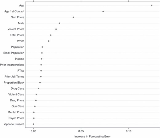
Predictor importance for forecasting skill
For Fig. 1, a charge of homicide or attempted homicide is being forecasted. The age of the individual on probation or parole is the most important variable. If age is not allowed to contribute to forecasting skill, forecasting error increases by about 12 percentage points (from 57% incorrectly forecasted to 69% incorrectly forecasted).
The age at which the individual has his or her first contact with the adult court system—an indicator of very serious behaviour for anyone under 18 years old—is the second most important predictor. Its contribution is about 8 percentage points. The number of prior convictions involving a firearm follows with a contribution of about 6 percentage points. Of somewhat less importance are, in order, gender, the number of prior convictions for violence offences, the total number of all prior convictions and race. The meaning of the other predictors is described briefly in Appendix B.
5.4. Partial response functions
In addition to learning something of each predictor’s contribution to forecasting skill, it can be useful to see how each predictor is related to the response variable when other predictors are held constant. In this instance, the sign and form of the response functions would need to make sense to stakeholders.
Such information can be provided by graphs such as Fig. 2, which shows a partial dependence plot for age. The horizontal axis is in units of years, and the vertical axis is in units of ‘centred logits’ that are generated as in expression (1) below. The small circles are the fitted values for the response committed or attempted homicide for different ages, holding all other predictors constant in a way that will be discussed. A smoother is overlaid.
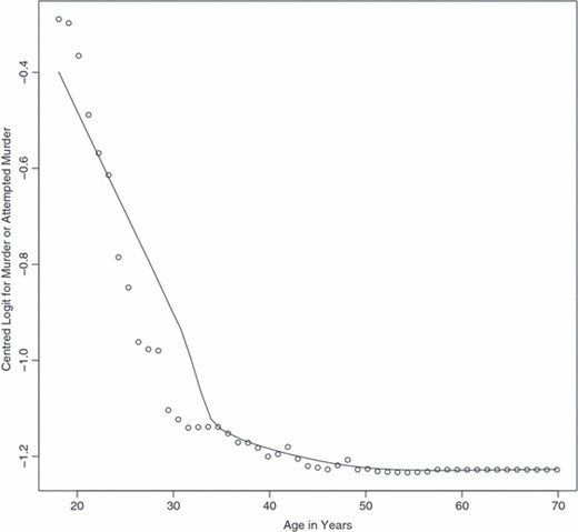
Partial dependence plot for age
Consider, for example, a given predictor X such as age. Suppose that there are M age values: X = 18,19,20,…, up to the Mth. For each value of X, in this case age, the fitted proportion of individuals in each category of the response is constructed from the random-forests output. In general the response may have K categories and expression (1) reflects this general situation. The homicide response here is binary with K = 2. Regardless of an individual’s age, all other predictor values are fixed at their existing values in the training data. As outlined in Appendix A.3, this is done by assigning each of the age values in turn to all individuals while leaving their other predictor values unchanged. In effect, one manipulates each individual’s age and nothing else before each of the fitted M proportions is computed. The M proportions are then used to implement equation (1) so that
where fk(X) is the response function value for response category k, for k = 1,2,…,K, the argument of X ranges over the M values of the predictor of interest and pk(X) is the fitted proportion for the kth category of the response given the value of X.
Thus, the vertical axis is the disparity between the fitted proportion for category k and the average of the fitted proportions for all K response categories in log-units. In this case, K is 2, and pk(X) is the fitted proportion of individuals who are forecasted to be charged with a homicide or an attempted homicide as a function of the set of available predictors or the fitted proportion of individuals who are not forecasted to be charged with a homicide or an attempted homicide as a function of the set of available predictors. A full discussion of partial dependence lots can be found in Hastie et al. (2001), pages 333–334.
From Fig. 2, it is apparent that the relationship between age and the log-odds of being charged with a homicide or attempted homicide is highly non-linear. The log-odds decline very rapidly from about age 18 years to about age 30 years. After age 30 years, the relationship is flat. A negative relationship was expected. A highly non-linear function of age was not. The message is clear: offenders in their late teens and early 20s are far more likely to be charged with a homicide or attempted homicide than offenders who are older than 30 years. Working backwards from the logit units, the probability of failure is about twice as large.
Fig. 3 shows that the age at which first contact is made with the adult court system also has a highly non-linear relationship with the response. There is a sharp decline from about age 12 years to about age 30 years and then the partial dependence plot begins a more gradual increase until age 50 years. Offenders who begin their criminal activities earlier are especially dangerous: the probability that they will be charged with a homicide or attempted homicide is larger by a factor of 2. One implication is that an aggravated assault, for example, committed at age 13 years is a strong predictor of later murderous conduct, although that same assault committed at age 30 years is not.
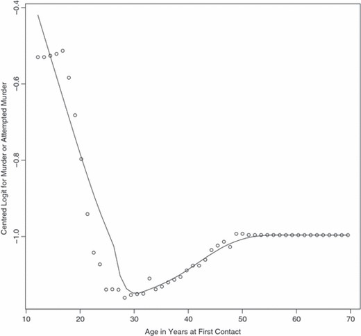
Partial dependence plot for age at first adult court contact
The increase in risk after age 30 years was unexpected. It may represent offenders who are engaged in domestic violence, which is almost by definition not possible until dating begins, can be exacerbated with cohabitation and often emerges after the peak years for other kinds of crime have passed. More generally, there may be a special aetiology for violence that is committed by people who begin their criminal activities relatively late in life.
Fig. 4 shows the partial dependence plot for the number of violent prior convictions. Again, the relationship is non-linear. The risks increase very dramatically from 0 to 2 violent prior convictions and increase strongly up to about 50 prior convictions. It can be important to appreciate that there can be a prior conviction for each charge that is associated with a given crime incident. For example, if there is an armed robbery of a convenience store, there could be a dozen charges. Over several crime incidents, these charges can accumulate rapidly. Offenders with more than 50 prior convictions for violent crimes are relatively rare but are real. That said, the relationship with the response is strong. The difference between an offender with no violent prior convictions and an offender with 10 violent prior convictions is approximately to double the probability that a homicide or attempted homicide will be charged. Very similar patterns were found for gun-related prior convictions.
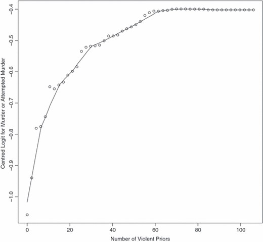
Partial dependence plot for the number of violent prior convictions
Fig. 5 shows the partial dependence plot for the size of the African-American population in an offender’s zip code area at time of intake. The response function is roughly S shaped. Up to about 20000 African-American residents, there is no relationship. Between about 20000 and 50000 African-American residents, the relationship is strongly positive. Above 50000 African-American residents, there is again no relationship. The effect on the odds of a homicide or attempted homicide charge is modest. The difference between 20000 and 50000 residents multiplies the probability by a factor of about 1.25.
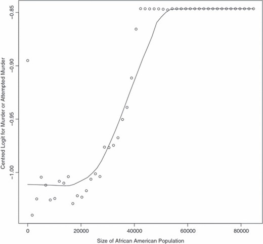
Partial dependence plot for the size of the African-American population
It is not clear how the relationship should be interpreted. At face value, we might think that the size of African-American population is a surrogate for the number of potentially violent offenders and the number of potential victims. But that would not explain the levelling off of the relationship when the size of the African-American population is very large.
Another interpretation of Fig. 5 is that the proportion of a zip code area that is African-American is the real predictor. However, among the variables that are held constant is the overall population of the zip code area. As a result, the role of the number of African-Americans plays out with the overall population size fixed. But that also is unsatisfying because it is well known that, in the USA, people tend to kill others like themselves; cross-race homicides are relatively rare. So, again, there is no apparent explanation for the levelling off on the right-hand side of the plot.
Moreover, the proportion African-Americans was included directly as a predictor. If there were to be neighbourhood effects as a function of race, this was the predictor that we thought would surface. It did not, and various combinations of neighbourhood variables all led back to the number of African-Americans.
Finally, median household income was one of the predictors that was included in the analysis. Typical household income is thus apparently not an explanation either. Nevertheless, we suspect that the number of African-Americans is a surrogate for one or more other neighbourhood variables that can affect crime, such as spatial concentration of poverty, offenders or even microlocal cultural patterns such as a sense of collective efficacy in informal social control (Sampson et al., 1997). How this admittedly modest association is to be explained will need to be explored in future research.
Partial dependence plots for the other quantitative predictors were not especially interesting. They summarized relationships that were not strong and approximately linear. Partial dependence plots for categorical predictors are generally of little help except to establish the direction of the association. Here, African American and male offenders were more likely commit homicides or attempted homicides.
In summary, one must be clear that the partial dependence plots are meant to be solely descriptive. There is no statistical model, causal or otherwise, in random forests. However, the signs of the relationships are broadly consistent with much past research and with social science theory that would give the associations causal interpretations. A major surprise is the number of highly non-linear associations. To the best of our knowledge, these non-linearities are new findings that no extant theory anticipates with any real precision. The non-linear relationships also help to explain why random-forests forecasts do so much better than logistic regression and other parametric regression procedures. In this instance, the parametric regression models got the functional forms very wrong because the actual functional forms were unknown when the data analysis began.
6. Discussion
In the overall pool of cases on probation or parole, the chances are about 1 in 100 that an individual will be charged with a homicide or an attempted homicide within 2 years after intake. For the subset of high risk cases that were identified by random forests, the chances are a little less than 8 in 100. An important consequence is that, for every true positive case identified, there will be about 12 false positive cases. If the marginal distribution alone were used, however, and our forecasts ignored, the error rate would be far worse: for every true positive there would be nearly 100 false positive cases. Employing random forests yields an eightfold forecasting improvement over the implicit assumption that anyone on probation or parole in Philadelphia is equally likely to commit homicidal acts.
Many would find the false positive rate far too high for imposing any retributive harm, punishment or additional restraint on an offender. Others would call attention to the presence of offender race in the model, along with other predictors. Both issues can raise considerable controversy over the use of such forecasts but must be addressed in the context of the on-going use of untested and subjective clinical forecasts.
African-Americans in Philadelphia have two major concerns about young black men in their community. One is the extraordinarily high levels at which they are incarcerated, relative to whites. The other is the very high rate at which they are murdered, relative to whites. Both facts also appear to be true of England and Wales, Australia and other nations with historic racial divisions in their populations. Without necessarily addressing the causes of these differences, recent policy discussions have moved to the question of what can be done to reduce these disparities most immediately.
Excessive incarceration rates of both blacks and whites arguably can be addressed by sufficiently accurate forecasts that many offenders pose little threat to public safety. If prosecutors, judges and parole boards could be reliably informed when an individual is no more likely to commit a violent crime than a person with no criminal record, they might have greater protection from the consequences of false negative forecasts (Anderson, 1995) and may be less likely to ‘overincarcerate’. The alternative, more risk averse, current practice relies on untested judgements and, when there seems to be any chance of a serious crime whatsoever, produces a decision to incarcerate.
There is no doubt of controversy that is associated with either approach. The choice may depend on one’s vision of the role of imprisonment in modern society. At one extreme is a high imprisonment society with unacknowledged forecasting errors from widespread (but unmeasured) use of false positive outcomes to prevent false negative outcomes. And still there will be some false negatives. At the other extreme is a low imprisonment society relying heavily on community supervision. There would probably be controversy over both false negative and false positive outcomes produced explicitly by the forecasting model. In short, the choice may lie between more incarceration with less controversy, or less incarceration with more controversy, playing out within the fiscal constraints that are imposed by taxpayers, their elected representatives and criminal justice administrators.
It does not seem adequate, as many law professors argue, that it is a better world without quantitative predictive tools. As long as subjective forecasts are used, or even required by statute, the problem of forecasting error will be with us. Ignoring the informal prediction algorithms that are now used does not make them go away. Unmeasured and undocumented racial bias may be just as much—or more—a component of untested clinical forecasting than of a statistical model in which race contributes a little to forecasting accuracy. The democratic virtue of a statistical forecast is that it is transparent and debatable.
For those who argue against the use of race in a multivariate model, our approach may be far more able to document racial effects, and in principle to remove them, than can clinical approaches. The very definition of ‘racial profiling’ in US law hangs on just such matters, as a recent report of the National Academy of Sciences has shown (Skogan and Frdyl, 2004). Some have argued that racial profiling consists of decisions that are made solely on the basis of race, but not on the use of race as one of many variables in a model that is used to inform decisions. Others have argued that any explicit use of race at all, no matter how minor a factor, is unacceptable. These choices are clearly about values but may also have empirical assumptions underlying them. The debate might be informed by additional facts.
In this analysis, we find that race improves forecasting skill, but not by much, in a population that is substantially African-American (approximately 65%). If the information that is contained in the racial variable is removed from the forecasts, forecasting error is increased by 2%. If the citizens of Philadelphia or their leaders prefer to take a small increase in forecasting error to gain a large improvement in the legitimacy of the entire process, that is exactly what an informed democracy can do. What should not be concluded from this discussion, however, is that the entire approach depends on the use of race. Just the opposite is true.
What the approach does depend on is the open acknowledgment of errors in forecasting, both false positive and false negative outcomes. How far such forecasts can or should be used in criminal justice is for others to decide. But it is instructive that Philadelphia judges have asked to have forecasts of homicide provided to them in making decisions about bail, which place about 6000 people behind bars and another 30000 people at large in the community while awaiting trial. Their view is that they could make much better decisions in such cases with these forecasts, just as probation chiefs can make better decisions about how much time and money to invest in any one of their cases.
It is also true that, with more investment in forecasting, the error rates will continue to go down. In particular, more can be done to obtain better data with which to construct forecasts. Among the data sets being sought in Philadelphia are juvenile records, as distinct from adult court records of offenders, containing information on juvenile criminal charges. Because the most dangerous felons often come to the attention of criminal justice officials at a very early age, juvenile records may contain information that is useful for forecasting adult probation or parole outcomes.
In a sense, the forecasts so far have been too good. Some identified probationers have committed new crimes so quickly that there was insufficient time to deliver any meaningful services to them. The reasons for these failures included not just homicides or attempted homicides, but a range of serious crimes. Also, two parolees were shot to death and one was shot several times at close range and lived. It will be an on-going challenge to intervene with the speed and intensity that are needed to keep these offenders healthy and out of trouble.
On the basis of our current forecasts, there is now a special unit within the APPD to oversee the individuals whom our procedures identify. At intake, the background variables of new cases are ‘dropped down’ the random-forests model to generate forecasts. If these individuals fall in the high risk group, they are eligible for the new special unit. There is a set of special services for the eligible individuals. Case-loads are under 20 so that the officer in charge can frequently have face-to-face contact with the parolees or probationers. Among the additional services are cognitive behavioural therapy for those who are diagnosed to need it and access to programmes that can improve health, literacy and job skills. As soon as the content of these services is clearly defined, and it is determined that they can be consistently delivered with high integrity, a randomized clinical trial can be mounted. Among the high risk offenders, some would be assigned at random to the usual forms of supervision. The others would be assigned at random to various combinations of special services. The question to be answered is whether there are cost-effective interventions for offenders at high risk of committing a homicide.
7. Conclusions
The APPD, like many such departments in large cities across the USA, has too few resources to provide proper oversight and services for those who might most benefit. One policy response can be to determine which offenders are in greatest need and then to devote a larger share of the resources to them. Offenders who are more likely to commit a homicide or attempted homicide might be one such group. The analyses that are presented in this paper would seem to provide a useful way to target scarce resources better. Whether these resources can be translated into cost-effective interventions is at this point unknown. Whether focusing supportive services on high risk offenders could prevent homicide remains an empirical question. Our forecast is that investing in one or more clinical trials would help to provide fairer and more effective policies for the prevention of homicide.
Although the focus of this paper is on forecasting murder in a population of offenders under community supervision, the methods that we use could have far broader application. The Virginia sentencing guidelines, for example, already use statistical recidivism forecasts in deciding whether or how long to incarcerate convicted offenders (Ostrom et al., 2002), the imposition of which has been followed by substantial reductions in the number of prisoners (Virginia Criminal Sentencing Commission, 2007). Yet in England and Wales, where the Criminal Justice Act of 2003 (part 12, chapter 5, sections 225–236) created ‘indeterminate sentences for public protection’ to keep ‘dangerous’ offenders in prison until they proved that they were safe to be released, no statistical criteria were provided for either imposing the sentence or releasing the offenders. In contrast with the declining custody rates with Virginia’s statistical approach, the English experience has seen a sharply rising prison population, with over 3000 (out of 82000) prisoners placed under indeterminate sentences for public protection in its first 2 years of operation.
It is impossible to anticipate accurately whether statistical forecasting of serious crime would result in more or less crime or imprisonment. All that we attempt to demonstrate in this paper is that recently developed statistical learning procedures can be used to forecast serious crime far more reliably than the procedures previously and at present used for such statistical forecasts. If useful forecasts can be made, scarce resources can be concentrated on the ‘power few’ subset of offenders who cause the greatest harm and public concern about crime (Sherman, 2007b). Such forecasts can be the first step of an increasingly widespread two-step approach: identifying important population subsets; then using randomized trials to develop and test the most cost-effective strategies for achieving beneficial objectives (Ayres, 2007).
Acknowledgements
Richard Berk’s work on this paper was funded by seed money from the University of Pennsylvania, and a grant from the National Science Foundation: SES-0437169, ‘Ensemble methods for data analysis in the behavioral, social and economic sciences’. Geoffrey Barnes’s work and Lawrence Sherman’s work were funded by the Jerry Lee Foundation. All of this support is gratefully acknowledged. Special thanks go to the Joint Editor and several reviewers for their very helpful suggestions.
References
Appendix A: The random-forests algorithms
Below are broad summaries of three important algorithms that are used by the version of random forests that we employed. These summaries are not substitutes for understanding the details of what the software actually does. For ease of exposition, some short-cuts have been taken and some details overlooked.
A.1. Random-forests algorithm summary
- (a)
There are N observations in the training data. Take a random sample of size n with replacement from the training data. (More complicated sampling approaches are available in some software to help to respond to special features of the analysis, such as asymmetric costs of false positive and false negative forecasts.) The observations selected are used to grow a classification tree. The observations that are not selected are saved as the OOB data. These can be test data for that tree and will on average be about a third of the full data set that is used in the analysis, i.e. the sample size of the OOB data will on average be about a third of N.
- (b)
Take a random sample of predictors. The sample is often very small (e.g. three predictors).
- (c)
Partition the data by using CART methods (as usual) into two subsets minimizing the Gini index.
- (d)
Repeat steps (b) and (c) for all subsequent partitions until further partitions do not improve the model’s fit.
- (e)
Compute (as usual) the class to be assigned to each terminal node.
- (f)
‘Drop’ the OOB data down the tree and assign the class that is associated with the terminal node in which an observation lands. The result is the predicted class for each observation in the OOB data for a given tree.
- (g)
Repeat steps (a)–(f) a large number of times to produce a large number of classification trees.
- (h)
For each observation, classify by majority vote over all trees when that observation was OOB. For example, if for 251 out of 500 trees a given case is classified as a ‘failure’, a failure is the class that is assigned to that case.
A.2. Variable importance algorithm summary
- (a)
As in Appendix A.1, compute the predicted class over all trees for each case in the OOB data.
- (b)
Compute the proportions of cases that are misclassified for each response class. These serve as measures of forecasting accuracy when all the predictors are used to construct the forecasts.
- (c)
Randomly permute the values of a given predictor over all observations.
- (d)
Compute again the predicted class for each case in the OOB data.
- (e)
Compute the proportions of cases that are misclassified for each response class. These serve as measures of forecasting accuracy when the given predictor is randomly shuffled.
- (f)
Compute the increase in the proportion misclassified as a measure of that variable’s importance for each response class.
- (g)
Repeat from step (c) for each predictor.
A.3. Partial dependence plot algorithm summary
The basic idea is to show how the average value of the response changes with changes in a given predictor, with all other predictors fixed at their observed values. In effect, the algorithm manipulates the value of each predictor in turn, but nothing else, and records what happens to the average response.
- (a)
For a given predictor with M values, construct M special data sets, setting the predictor values to each value m in turn and fixing the other predictors at their existing values. For example, if the predictor is years of age, M might be 20, and there would be 20 data sets, one for each year of 20 years of age. In each data set, age would be set to one of the 20 age values for all observations (e.g. 18 years old), whether that age was true or not. The rest of the predictors would be fixed at their existing values.
- (b)
Using a constructed data set with a given m (e.g. 22 years of age) and the random-forests output based on the steps that are summarized in Appendix A.1, compute the predicted class (here, failure or not) for each case.
- (c)
Compute the proportion of failures over all cases.
- (d)
Compute the logit from this proportion. These are not conventional logit units because they are centred on the average of the two (in this case) proportions of the response category. They are analogous to how in analysis of variance the effects of different levels of a treatment are defined; their effects sum to 0. Here, the rationale is that we must anticipate the case when there are more than two response categories and it is not likely to be apparent how we should choose the reference category for a log-odds.
- (e)
Repeat steps (b)–(d) for each of the M values.
- (f)
Plot the logits from step (d) for each m against the M values of the predictor.
- (g)
Repeat steps (a)–(f) for each predictor.
Appendix B: Additional predictor definitions
- (a)
‘population’ is the number of people living in the offender’s zip code area.
- (b)
‘black population’ is the number of African-Americans living in the offender’s zip code area.
- (c)
‘income’ is the median household income in the offender’s zip code area.
- (d)
‘prior incarcerations’ is the number of prior incarcerations in state prisons.
- (e)
‘FTA’ is the number of times that the offender failed to show for a court appearance.
- (f)
‘prior jail terms’ is the number of prior jail terms.
- (g)
‘proportion black’ is the proportion of the population that is African-American in the offender’s zip code area.
- (h)
‘drug case’ is whether the instant offence was drug related.
- (i)
‘violent case’ is whether the instant case was violence.
- (j)
‘drug priors’ is the number of prior convictions for drug offences.
- (k)
‘gun case’ is whether the instant offence involved the use of a firearm gun.
- (l)
‘mental priors’ is the number of prior mental health probation or parole cases implying assignment to the special mental health unit.
- (m)
‘psych priors’ is the number of prior probation or parole cases in which a psychiatric condition was imposed.
- (n)
‘zipcode present’ is whether there was a reported home address for an offender from which the zip code could be determined.
Some of these predictors are highly correlated but, because the algorithm samples predictors, there are usually not serious problems.
