


Abstract
Likelihood-based methods of inference of population parameters from genetic data in structured populations have been implemented but still little tested in large networks of populations. In this work, a previous software implementation of inference in linear habitats is extended to two-dimensional habitats, and the coverage properties of confidence intervals are analyzed in both cases. Both standard likelihood and an efficient approximation are considered. The effects of misspecification of mutation model and dispersal distribution, and of spatial binning of samples, are considered. In the absence of model misspecification, the estimators have low bias, low mean square error, and the coverage properties of confidence intervals are consistent with theoretical expectations. Inferences of dispersal parameters and of the mutation rate are sensitive to misspecification or to approximations inherent to the coalescent algorithms used. In particular, coalescent approximations are not appropriate to infer the shape of the dispersal distribution. However, inferences of the neighborhood parameter (or of the product of population density and mean square dispersal rate) are generally robust with respect to complicating factors, such as misspecification of the mutation process and of the shape of the dispersal distribution, and with respect to spatial binning of samples. Likelihood inferences appear feasible in moderately sized networks of populations (up to 400 populations in this work), and they are more efficient than previous moment-based spatial regression method in realistic conditions.
Introduction
Accurate estimation of dispersal in natural populations by demographic observations is difficult, which has led to the development of many methods to infer dispersal from genetic information. Recent developments include some applications of assignment techniques (Wilson and Rannala 2003, Paetkau et al. 2004, Faubet and Gaggiotti 2008), methods based on simulation of the distribution of summary statistics (such as so-called approximate Bayesian computation, e.g., Beaumont 2007 applied to dispersal estimation in Hamilton et al. 2005 and Becquet and Przeworski 2007) and likelihood methods (Rannala and Hartigan 1996, Beerli and Felsenstein 1999, Beerli and Felsenstein 2001, de Iorio and Griffiths 2004b) that aim to use all information in the data.
These methods seem to perform well for low migration rates between a small number of populations, but their performance is more generally uncertain. For example, the evaluation of likelihood remains time consuming, so that likelihood methods have been tested only for small networks of populations, and the reliability of the computations is sometimes debated (Abdo et al. 2004, Beerli 2006). Further, all methods may rest on questionable assumptions. For example, it has been found that “ghost” populations unaccounted in the statistical model can affect maximum-likelihood (ML) estimation of dispersal and mutation parameters of sampled populations (Beerli 2004, Rousset and Leblois 2007). Thus, perennial questions (e.g., Cox 2006, p. 170) about the benefits of likelihood analyses relative to alternative methods remain pending.
Application of full-likelihood methods to the scenario of localized dispersal or “isolation by distance,” relevant for many ecological studies, has only been considered in Rousset and Leblois (2007), and alternative methods are still being developed (e.g., rare allele methods, Novembre and Slatkin 2009). Rousset and Leblois (2007) described the properties of point estimates of dispersal and mutation parameters in linear habitats. The evaluation of likelihood was based on the algorithms of de Iorio and Griffiths (2004b). As evaluation of likelihood performance was time consuming, a fast heuristic approximation known as product of approximate conditional likelihood (PAC-likelihood, Li and Stephens 2003) was also considered. Inferences from PAC-likelihood surfaces appeared practically as efficient (precise) as full-likelihood inferences, even though the PAC-likelihood is a biased estimate of the likelihood for each parameter point. In the present work, these results are extended to two-dimensional habitats. Further, the performance of likelihood-based confidence intervals is analyzed.
The following general features are shared with and further discussed in Rousset and Leblois (2007): Allelic type data will be considered, with microsatellite data as the intended subject of application. We envision many species as spatial clusters of subpopulations with large immigration probabilities within each cluster, and less dispersal among clusters, and we are interested in the analysis of one such cluster. Its structure is described as a regular array of demes of size N for which we estimate the following parameters: a mutation rate, a number of immigrants per deme (Nm), and a dispersal scale parameter (that of a geometric distribution). We also consider the neighborhood size or equivalently the product of population density and mean square dispersal distance, the latter being a function of the two previous parameters. We will compare performance of neighborhood estimation to that of variants of the method based on regression of estimates to geographical distance (e.g., Rousset 1997, Watts et al. 2007).
Evaluation of performance involves both evaluation under ideal conditions where the data are generated under the model used as a basis for statistical analysis and evaluation of robustness under model misspecification (e.g., Casella and Berger 2002, p. 481). In this paper, we consider both steps. We first evaluate performance under nearly ideal conditions (known mutation model, known dispersal distribution), in particular to demonstrate that we have an effective implementation of likelihood inferences. Overall, the estimation performance may be considered excellent, with good coverage of the confidence intervals, and generally small biases and small mean square errors. We nevertheless obtain some nonideal results and show that they are inherent to the statistical method rather than a feature of our implementation. More specifically, the algorithm used to estimate likelihood is based on coalescent approximations, that is, approximations for large deme size, small migration, and small mutation probability. When applied to samples from finite-sized populations, the statistical model thus always appears misspecified except in the case of vanishing migration rate between arbitrarily large populations, a case that may be of limited practical interest. The coalescent approximation affects the results, as estimates of dispersal parameters (number of migrants and the shape parameter of the dispersal distribution) are biased when the dispersal probability is large. Neighborhood estimation may be more robust in this respect. We also compare strict likelihood and PAC-likelihood inferences and find that their performance are practically equivalent.
In a second step, we evaluate performance of PAC-likelihood inferences under conditions including misspecification of the dispersal distribution and of mutation model, and otherwise designed to approximate realistic conditions, based on the study of damselfly populations by Watts et al. (2007). We consider the effect of spatial binning of samples, as such binning is necessary to fit data from individuals that can be sampled from anywhere in continuous space, to the framework of the statistical model that assumes a regular grid of demes. As computations are also faster for small arrays of demes, a coarse-grained spatial binning of samples can also reduce the computation load compared with a fine-grained one. But it can also induce biases or results that are difficult to interpret. Finally, we compare neighborhood size estimation to that achieved by previous methods and conclude that likelihood-based estimation can perform better in practical conditions.
Methods
For each simulated data set, the analysis goes through three main steps, implemented in the software Migraine and further described in the Appendix. First, likelihoods are estimated, with some error, for a number of parameter points. Next, a likelihood surface is inferred from the likelihood points by a classical smoothing method (Kriging). Third, parameter values of interest (the mutation and dispersal parameters used to generate the data) are tested by profile likelihood ratio tests (profile LRTs, e.g., Cox and Hinkley 1974, Severini 2000). Profile LRTs also allow the construction of profile likelihood confidence intervals. Ideally, the main measures of the quality of inference are the coverage properties of such confidence intervals for given parameter values. Note that this differs from coverage averaged over a prior distribution of parameter values, as measured in some studies (Beerli 2006, Hey 2010, Peter et al. 2010). Only the demonstration of good coverage for fixed parameter values ensures good average coverage for any imperfectly known prior distribution or for any prior information in the form of a likelihood surface. The coverage properties of confidence intervals, for given parameter values, can be assessed through the distribution of the P value of the corresponding profile LRTs. Ideally, this distribution is uniform; but this comfortable ideal is rarely attained in practice and then some consideration of the practical importance of the biases is useful in assessing the method.
In this section, we detail the basic assumptions of the sample simulation model and of the statistical model. In the Appendix, we further detail the implementation of the statistical model and the method of inference of likelihood surfaces.
Dispersal Models for Sample Simulation
Samples have been simulated by the IBDsim program (Leblois et al. 2009). Two dispersal distributions have been considered, a geometric dispersal model similar to the one of the statistical model and the Poisson reciprocal gamma model (Chesson and Lee 2005). The latter distribution is Gaussian-looking at short distances, but power-tailed, and can therefore have a high kurtosis. Its two parameters and κ determine the power of the tail, and the second moment . We vary in our simulations by varying κ for fixed , whereby the axial kurtosis varies between 20.1 and 22.5.
Exact Control of Number of Migrants
Absorbing boundaries are assumed, so that the demes near edges typically receive fewer immigrants since they have fewer close neighboring demes. The actual number of immigrants thus differs from the number of emigrants deduced from the forward distribution. Such discrepancies are easily detected by the statistical estimation of number of immigrants. Then, one needs to control the number of immigrants in the sample simulation rather than simply let it be a complex function of the forward distribution and of habitat edge effects. Hence, in both sample simulations based on the geometric distribution and in statistical analysis, the Nm parameter is defined to give the maximal (over demes) expected number of immigrants in a deme whatever the edge effects. This differs from simulations in Rousset and Leblois (2007) and will be included as an option in future versions of the IBDsim program. On the other hand, no attempt was made to control Nm values in our sample simulations based on the Poisson reciprocal gamma distribution. In the latter simulations, the immigration rate in most demes was , a situation where no demic structure would be recognized in practice.
Geometric Dispersal
The scale parameter g describes the geometric decrease, with distance between demes, of the pairwise forward immigration probabilities. In two dimensions, forward probabilities decrease according to relative values of , x and y being the axial dispersal distances in each dimension (not both zero), and if and otherwise (Kronecker's notation). As described above, the forward dispersal probability is adjusted such that the maximal expected number of immigrants in a deme has a known preset value and that the deme of origin of immigrants is chosen according to the relative values of the forward dispersal probabilities.
The Neighborhood Parameter
Dispersal in the Statistical Model
A geometrical dispersal model is assumed in likelihood computations. Its exact meaning differs from that of the geometrical dispersal model assumed in sample simulations. In the likelihood computations, g describes the decrease of the expected number of immigrants with distance, whereas in the sample simulation, g describes the decrease in forward immigration rates. Such discrepancies cannot be generally avoided because the likelihood computations are based on a limit process where all dispersal probabilities among different demes are infinitesimally small and considers only one parameter Nm where the sample simulation considers the two parameters N and m separately.
In particular, the edge effects cannot be treated identically in both algorithms. In the likelihood computations, we assumed the number of immigrants between pairs of demes is a function of their relative position only and not of their position relative to the edge of the habitat; whereas in the sample simulation algorithm, it is determined by computation of backward dispersal probabilities from forward probabilities (as is usual), and this depends on the position of the two demes relative to the edges of the lattice. Further details and a numerical example are given in the Appendix, illustrating that the discrepancies between the two algorithms may be small.
Mutation Models
The default mutation model considered in sample simulations was a symmetric K-alleles model (KAM) with 10 alleles. A one-step stepwise mutation model (SMM), also with 10 alleles, was also considered in some sample simulations. The KAM was assumed in all likelihood computations.
Sampling Design
Two-hundred data sets are analyzed for each simulation condition. Each data set includes 10 independent loci. In the two-dimensional case, square habitats of or populations are simulated, and 10 diploid individuals are sampled at each of 8 demes, two in each corner, that is, at positions (1,1) and (2,2) in one corner and symmetrically in the other corners. In this way, both adjacent and distant populations are sampled, which should facilitate estimation of the scale of dispersal. On the other hand, this design may highlight edge effects. In linear-habitat cases, samples of 10 individuals were taken in each subpopulation for arrays of four populations; at positions 2–8 (or 2–16, cases [5], [6], [25], [26]) by steps of 2 for 16 populations; and at positions 40–58 by steps of 2 for 100 populations.
Results
Minimal Misspecification
Full Likelihood
The correctness of the confidence intervals can be examined graphically by looking whether the empirical cumulative distribution function of P values aligns (or not) with a 1:1 diagonal line. These distributions are shown for all simulation conditions in the Supplementary Material online for details. Figure 1 (left) illustrates a good result. Deviations from the diagonal are tested by the Kolmogorov–Smirnov test (“KS” inset in each subplot). Four subplots are presented, one for each of the canonical parameters and one for . Also shown below each subplot are the relative (except for g) bias and root mean square error (RMSE) of each ML estimator (the same numbers are reported in table 1, case [1]). It may be observed, and this will also be true when confidence intervals have incorrect coverage that the bias and RMSE of and Nm are small by practical standards. The relative bias and RMSE can be very large. This will typically occur when the data show no evidence of isolation by distance (and therefore when arbitrarily large estimates may be obtained). In general, the distribution of estimates is much closer to Gaussian, which make comparisons of bias and RMSE more meaningful. For this reason, the relative bias and relative RMSE reported in figures and tables are those of 1/Nb.
Performance of Estimation by Strict Likelihood
| Parameters | Relative Nμ | Relative Nm | g | Relative 1/Nb | |||||||||||||
| Array | N | m | g | μ | Bias | RMSE | KS Test | Bias | RMSE | KS Test | Bias | RMSE | KS Test | Bias | RMSE | KS Test | |
| [1] | 4 × 4 | 400 | 0.01 | 0.5 | 5 × 10⁻⁴ | 0.028 | 0.16 | 0.28 | 0.05 | 0.17 | 0.29 | 0.012 | 0.16 | 0.81 | 0.059 | 0.71 | 0.96 |
| [2] | 4 × 4 | 400 | 0.1 | 0.5 | 5 × 10⁻⁴ | 0.013 | 0.16 | 0.14 | 0.45 | 0.9 | 0.0021 | -0.00013 | 0.4 | 0.001 | 0.56 | 1.81 | 0.15 |
| [3] | 4 × 4 | 40,000 | 0.001 | 1 | 5 × 10⁻⁶ | 0.023 | 0.16 | 0.61 | 0.18 | 0.59 | 0.75 | ||||||
| [4] | 4 × 4 | 80 | 0.5 | 1 | 0.0025 | 0.02 | 0.16 | 0.79 | 2.26 | 2.6 | 0 | ||||||
| [5] | 16 | 40 | 0.25 | 0.25 | 0.001 | 0.0091 | 0.17 | 0.52 | 0.94 | 1.09 | 0 | -0.16 | 0.2 | 0 | -0.07 | 0.2 | 0.29 |
| [6] | 16 | 40,000 | 0.00025 | 0.25 | 1 × 10⁻⁶ | 0.011 | 0.18 | 0.21 | 0.15 | 0.41 | 0.99 | -0.023 | 0.14 | 0.78 | -0.0038 | 0.25 | 0.89 |
| [7] | 16 | 400 | 0.01 | 0.25 | 0.001 | 0.018 | 0.15 | 0.2 | 0.061 | 0.26 | 0.05 | -0.0055 | 0.14 | 0.39 | 0.013 | 0.33 | 0.62 |
| [8] | 16 | 400 | 0.01 | 0.5 | 0.001 | 0.041 | 0.17 | 0.63 | 0.069 | 0.19 | 0.058 | -0.017 | 0.11 | 0.097 | 0.074 | 0.45 | 0.38 |
| [9] | 4 × 4 | 400 | 0.01 | 0.25 | 0.001 | 0.055 | 0.19 | 0.022 | 0.04 | 0.19 | 0.072 | 0.0066 | 0.16 | 0.31 | 0.04 | 0.5 | 0.83 |
| [10] | 4 × 4 | 400 | 0.01 | 0.5 | 0.001 | 0.045 | 0.18 | 0.2 | 0.034 | 0.17 | 0.42 | -0.0021 | 0.16 | 0.79 | 0.18 | 0.89 | 0.71 |
| [11] | 4 × 4 | 400 | 0.01 | 0.75 | 0.001 | 0.022 | 0.17 | 0.11 | 0.051 | 0.18 | 0.44 | 0.0027 | 0.19 | 0.0052 | 0.75 | 2.51 | 0.0029 |
| [12] | 4 | 400 | 0.01 | 1 × 10⁻⁴ | 1 × 10⁻⁴ | – 9 × 10⁻⁴ | 0.17 | 0.31 | -0.0079 | 0.22 | 0.58 | 0.056 | 0.12 | 0 | -0.096 | 0.27 | 0.83 |
| [13] | 4 × 4 | 400 | 0.01 | 1 × 10⁻⁴ | 0.001 | 0.039 | 0.18 | 0.18 | -0.028 | 0.14 | 0.2 | 0.048 | 0.096 | 0 | -0.098 | 0.23 | 0.34 |
| [14] | 4 × 4 | 40,000 | 0.001 | 0.5 | 5 × 10⁻⁶ | 0.02 | 0.16 | 0.57 | 0.22 | 0.68 | 0.58 | 0.007 | 0.35 | 0.32 | 0.52 | 1.66 | 0.31 |
| [15] | 4 × 4 | 40 | 0.05 | 0.25 | 0.001 | 0.023 | 0.18 | 0.53 | 0.11 | 0.23 | 0.56 | 0.016 | 0.15 | 0.49 | -0.064 | 0.44 | 0.066 |
| [16] | 4 × 4 | 40 | 0.05 | 0.5 | 0.001 | 0.029 | 0.19 | 0.21 | 0.14 | 0.25 | 0.0098 | 0.0062 | 0.17 | 0.85 | 0.034 | 0.69 | 0.81 |
| [17] | 16 | 400 | 0.01 | 0.75 | 0.001 | 0.025 | 0.18 | 0.017 | 0.029 | 0.14 | 0.16 | -0.0056 | 0.081 | 0.76 | 0.13 | 0.67 | 0.96 |
| [18]a | 100 | 40 | 0.5 | 0.5 | 5 × 10⁻⁴ | 0.045 | 0.17 | 0.29 | 2.39 | 2.73 | 0 | -0.28 | 0.31 | 1 × 10⁻⁹ | -0.06 | 0.24 | 0.53 |
| [19] | 10 × 10 | 400 | 0.01 | 0.5 | 5 × 10⁻⁵ | 0.027 | 0.16 | 0.75 | 0.0092 | 0.15 | 0.019 | 0.0034 | 0.093 | 0.53 | 0.033 | 0.4 | 0.99 |
| [20] | 4 × 4 | 400 | 0.01 | 0.99999 | 0.001 | 0.041 | 0.19 | 0.34 | 0.073 | 0.17 | 0.076 | -0.051 | 0.1 | 2.5 × 10⁻⁸ | 1.3 × 10⁸ | 4.4 × 10⁸ | 5.9 × 10⁻⁹ |
For case [80], only 30 samples were analyzed.
![Distributions of P values of likelihood ratio tests in cases [1] (left) and [2] (right).](https://oup.silverchair-cdn.com/oup/backfile/Content_public/Journal/mbe/29/3/10.1093_molbev_msr262/2/m_molbiolevolmsr262f01_ht.jpeg?Expires=1716534770&Signature=C0WXliGneTyChgA3RjndySjlfbPxLhDDhGFVRZpYQAqnT4Xk3AIdZBGKpoZN0Zpisu4Xr8huuuGDzh4KvvYsYfKfVSKNureTwZhJzSW~gSYBxGWoB4kmpHwK8JDai0gLDc61~eyFV3L4KO7J9Jfrsupi5xDeAqDFHIzdHl2tm6DXFqKD4dk4PBrOy8B9z34HrxKxs-H1MlXb-uCSKcz2YPyolk1daHMc7fb7cMIQsVlikHrN2QUu6nveDkovoZO1BVbM3cPfggU4PqPJ2BLVU41FzWETSSnLkFu-jxGDcERlW6Gz7bnXrHgqP9-7WuMYWztm7BC1aYBWPNLlHnsf~Q__&Key-Pair-Id=APKAIE5G5CRDK6RD3PGA)
Distributions of P values of likelihood ratio tests in cases [1] (left) and [2] (right).
Figure 1 (right; case [2] in table 1) presents a less satisfying result. The only difference with the previous example is that m is 0.1 rather that 0.01. In this and further simulations, there are three possible sources of nonideal performance inherent to the statistical model: 1) departure from coalescence assumptions (m being large or N being small); 2) spatial edge effects: They are expected when m is large, and g is intermediate (for low g, immigration probabilities are affected only in the outermost demes; for , the sample simulation model and the statistical model are the island model, both with the same immigration rate, so the edge effects are correctly specified). For given number of demes, edge effects should also be most visible in two-dimensional lattices because a higher fraction of populations are at the edge of the habitat; 3) estimates are at the boundary of the parameter space. This can occur for g and then the expected distribution of LRT P values is not uniform. Not only LRTs for g but also for other parameters can be affected (Self and Liang 1987).
The first two effects should disappear as N increases and m, μ decrease for fixed Nm, . The first effect (departure from coalescent assumptions for high m) is best singled out under an island model, that is, when g is fixed to 1 in sample simulation and in statistical analyses. These simulations clearly show better inferences of a fixed Nm value with N increasing from 80 to 40,000 and m decreasing from to (cases [3] vs. [4]). To illustrate what these changes in RMSE mean, fig. 2 shows the likelihood surfaces for the samples that yielded departures from parameter values closest to the RMSE values and of the same sign as the bias.
![Examples of likelihood surfaces for cases [3] (top) and [4] (bottom). The surfaces are inferred from 1,024 points as described in the Appendix. In both cases, the parameter values where 2Nμ=0.4 and 2Nm=80, but the bottom case illustrates the much higher RMSE of 2Nm estimates for low N, large m cases. The likelihood surface is shown only for parameter combinations that fell within the envelope of parameter points for which likelihoods were estimated. The cross denotes the maximum.](https://oup.silverchair-cdn.com/oup/backfile/Content_public/Journal/mbe/29/3/10.1093_molbev_msr262/2/m_molbiolevolmsr262f02_ht.jpeg?Expires=1716534770&Signature=nednscyzODWFZdLrjGpBilBC-I8RTnBDnea4GoGLZMo-5MkGJlaTKuZ~HfNXe4jCLytoyXr7F3pelGA~DzjylBw30s9yq8YqeSesO638OPnAnBkUI19G83eQbtFuLrtygAtQTVL8VHeGD8gNhXkiUqme6XzP2a9dHDfuxsddStJC2VWz9nwHaQdRh3n8KVY5kYjpxwQXq-ZUHKYrVPaj~ZWzJvoqNZCOim5E3QDbiIu9Ack~xgpZY8V5ih24Uh5N~CAeKc28yLxQMGQNNMpq3dc~EdCN1QG8SCGUwk6xkSkQzOc~TziucELrsa07Z96cGpCSzErgISz4zHDVKWJkpg__&Key-Pair-Id=APKAIE5G5CRDK6RD3PGA)
Examples of likelihood surfaces for cases [3] (top) and [4] (bottom). The surfaces are inferred from 1,024 points as described in the Appendix. In both cases, the parameter values where and , but the bottom case illustrates the much higher RMSE of estimates for low N, large m cases. The likelihood surface is shown only for parameter combinations that fell within the envelope of parameter points for which likelihoods were estimated. The cross denotes the maximum.
Under isolation by distance, the effect of the coalescent approximation is illustrated by comparison of cases [14] and [2] (N increasing from 40 to 40,000) and by comparison of cases [5] and [6] (N increasing from 400 to 40,000), although in both comparisons the third effect (g estimates at the boundary) may also affect performance more strongly when m is larger. Figure 3 shows the convergence of distributions of P values to uniform distributions in the last comparison. The same convergence is observed is the two previous comparisons (see Supplementary Material online for distributions of P values).
![Convergence of distributions of P values for increased N. The two cases differ only in N, m, and μ values for identical Nm and Nμ. N=40 (case [5]) on the left and 40,000 (case [6]) on the right.](https://oup.silverchair-cdn.com/oup/backfile/Content_public/Journal/mbe/29/3/10.1093_molbev_msr262/2/m_molbiolevolmsr262f03_ht.jpeg?Expires=1716534770&Signature=kyB-xek3atccAfkx88aqJ1nA4PGfnW3p8wb9PuByW8PXUg0jLp7NEdr3pyMICB~VPQLeFn3J0erArTsvmCXnkU3ymUYjACtOm8op9nbwGlRAGVYB0WCtk2mY7GWibvT22P1~rohKH~wVOySKiVqk-~XBQQ1XVqY2Vu75mZsDzeUBng7LJyhZ46quwUoWnz6rdFz8B60OlxWi8IttxRX3T4V0DW-1bUBZbX64U-gZLhA0Vle~pyW0JumF9hae7c2Z0Ud3NTPUvV~TGGP~Z83xZuv3rXI0SQwd8YE5SoxMfUPHef9JCWmb4gQdLy4dohhhqExEXanVveDptg14UvDgig__&Key-Pair-Id=APKAIE5G5CRDK6RD3PGA)
Convergence of distributions of P values for increased N. The two cases differ only in N, m, and μ values for identical Nm and . (case [5]) on the left and 40,000 (case [6]) on the right.
We can roughly rank different simulations according to the expected magnitude of the different effects from lowest to highest. Low m values are illustrated by cases [7]–[13] and [19], and the estimator biases are indeed small.
For (stepping stone model, cases [12] and [13]), the distribution of the LRT for is expectedly not uniform. The theoretical asymptotic distribution of the LRT P value is a mixture 1:1 of a with 1 degree of freedom and of a probability mass at 0. The observed mass at 0 actually departs from 1/2 (see cases [12] and [13] in Supplementary Material online for details), which is a general phenomenon (e.g., Pinheiro and Bates 2000, p. 87; Hey 2010). The profile LRTs for the other parameters appear unaffected, but this is not a general expectation (Self and Liang 1987).
When g approaches 1 (and neighborhood size approaches infinity), the same parameter boundary effects on g are encountered (case [20]; similar results are also obtained with 50 loci by PAC-likelihood, not shown). Further, numerical issues affect tests of large values of the neighborhood size ( for ). A way to circumvent this problem is to change the scale of uniform sampling of parameter points and of Kriging (i.e., uniform sampling of , see Appendix). Although this solves most of the numerical issues, the distribution of P values for Nb is distorted in the same way as that for g.
Conversely, the highest biases are expected for high m values (fig. 4). The largest Nm bias in tables 1 and 2 is for in a linear array of 100 demes (case [18]), and other cases with show large distortions of the distribution of P values. For intermediate m values () relatively large Nm biases may still be observed, but distorsions of P value distributions are generally less obvious, except in some cases where misspecification of spatial edge effects can also contribute (in particular, case [16]).
Performance of Estimation by PAC-likelihood
| Parameters | Relative Nμ | R | g | Relative 1/Nb | |||||||||||||
| Array | N | m | g | μ | Bias | RMSE | KS Test | Bias | RMSE | KS Test | Bias | RMSE | KS Test | Bias | RMSE | KS Test | |
| [21] | 4 × 4 | 400 | 0.01 | 0.5 | 5 × 10⁻⁴ | -0.026 | 0.16 | 0.1 | 0.039 | 0.17 | 0.64 | -0.004 | 0.16 | 0.78 | 0.18 | 0.82 | 0.77 |
| [22] | 4 × 4 | 400 | 0.1 | 0.5 | 5 × 10⁻⁴ | 0.0042 | 0.16 | 0.05 | 0.43 | 0.9 | 0.0012 | -0.015 | 0.41 | 0.00015 | 0.69 | 1.94 | 0.014 |
| [23] | 4 × 4 | 40,000 | 0.001 | 1 | 5 × 10⁻⁶ | 0.015 | 0.15 | 0.38 | 0.14 | 0.56 | 0.94 | ||||||
| [24] | 4 × 4 | 80 | 0.5 | 1 | 0.0025 | 0.016 | 0.16 | 0.84 | 2.2 | 2.55 | 0 | ||||||
| [25] | 16 | 40 | 0.25 | 0.25 | 0.001 | -0.016 | 0.17 | 0.96 | 0.85 | 1 | 0 | -0.17 | 0.2 | 0 | -0.012 | 0.2 | 0.16 |
| [26] | 16 | 40,000 | 0.00025 | 0.25 | 1 × 10⁻⁶ | -0.022 | 0.17 | 0.24 | 0.11 | 0.38 | 0.3 | -0.034 | 0.14 | 0.89 | 0.072 | 0.27 | 0.95 |
| [27] | 16 | 400 | 0.01 | 0.25 | 0.001 | -0.034 | 0.14 | 0.068 | 0.03 | 0.23 | 0.41 | -0.018 | 0.14 | 0.53 | 0.088 | 0.38 | 0.71 |
| [28] | 16 | 400 | 0.01 | 0.5 | 0.001 | -0.015 | 0.16 | 0.54 | 0.043 | 0.17 | 0.39 | -0.022 | 0.11 | 0.25 | 0.12 | 0.5 | 0.39 |
| [29] | 4 × 4 | 400 | 0.01 | 0.25 | 0.001 | -0.0022 | 0.17 | 0.15 | 0.027 | 0.18 | 0.067 | -0.0045 | 0.16 | 0.89 | 0.11 | 0.55 | 0.28 |
| [30] | 4 × 4 | 400 | 0.01 | 0.5 | 0.001 | -0.0049 | 0.17 | 0.33 | 0.023 | 0.16 | 0.89 | -0.011 | 0.17 | 0.94 | 0.27 | 1.01 | 0.79 |
| [31] | 4 × 4 | 400 | 0.01 | 0.75 | 0.001 | -0.022 | 0.17 | 0.066 | 0.04 | 0.19 | 0.43 | -0.00036 | 0.2 | 0.0034 | 0.92 | 2.9 | 0.0043 |
| [32] | 4 | 400 | 0.01 | 1 × 10⁻⁴ | 1 × 10⁻⁴ | -0.01 | 0.17 | 0.51 | -0.034 | 0.22 | 0.61 | 0.055 | 0.12 | 0 | -0.068 | 0.27 | 0.94 |
| [33] | 4 × 4 | 400 | 0.01 | 1 × 10⁻⁴ | 0.001 | -0.023 | 0.16 | 0.0042 | -0.053 | 0.14 | 0.46 | 0.041 | 0.088 | 0 | -0.054 | 0.22 | 0.021 |
| [34] | 4 × 4 | 40,000 | 0.001 | 0.5 | 5 × 10⁻⁶ | 0.012 | 0.16 | 0.66 | 0.2 | 0.67 | 0.62 | 0.0025 | 0.36 | 0.56 | 0.63 | 1.83 | 0.21 |
| [35] | 4 × 4 | 40 | 0.05 | 0.25 | 0.001 | -0.048 | 0.17 | 0.23 | 0.096 | 0.23 | 0.56 | -0.0097 | 0.15 | 0.25 | 0.053 | 0.49 | 0.7 |
| [36] | 4 × 4 | 40 | 0.05 | 0.5 | 0.001 | -0.036 | 0.18 | 0.2 | 0.13 | 0.24 | 0.024 | -0.011 | 0.18 | 0.78 | 0.16 | 0.81 | 0.27 |
| [37] | 16 | 400 | 0.01 | 0.75 | 0.001 | -0.023 | 0.17 | 0.0052 | 0.014 | 0.13 | 0.21 | -0.008 | 0.081 | 0.55 | 0.17 | 0.69 | 0.72 |
| [38] | 100 | 40 | 0.5 | 0.5 | 5 × 10⁻⁴ | -0.13 | 0.22 | 5.3 × 10⁻¹³ | 2.37 | 2.57 | 0 | -0.29 | 0.32 | 0 | -0.029 | 0.23 | 0.43 |
| [39] | 10 × 10 | 400 | 0.01 | 0.5 | 5 × 10⁻⁵ | -0.16 | 0.2 | 1.1 × 10⁻¹⁶ | -0.0092 | 0.14 | 0.011 | -0.029 | 0.12 | 0.12 | 0.28 | 0.64 | 0.19 |
| [40]a | 4 × 4 | 400 | 0.01 | 0.99999 | 0.001 | -0.0027 | 0.18 | 0.022 | 0.06 | 0.16 | 0.16 | -0.052 | 0.1 | 5 × 10⁻⁷ | 1.3 × 10⁸ | 4.2 × 10⁸ | 2.9 × 10⁻⁷ |
| [41] | 10 × 10 | 400 | 0.01 | 0.5 | 5 × 10⁻⁴ | 0.11 | 0.47 | 0.72 | -0.032 | 0.14 | 0.56 | -0.026 | 0.15 | 0.44 | 0.52 | 1.82 | 0.38 |
| [42] | 10 × 10 | 400 | 0.1 | 0.5 | 5 × 10⁻⁴ | 0.014 | 0.22 | 0.5 | 0.14 | 0.47 | 0.26 | 0.011 | 0.25 | 0.53 | 0.17 | 0.9 | 0.99 |
| [43] | 10 × 10 | 400 | 0.01 | 0.75 | 5 × 10⁻⁴ | 0.12 | 0.49 | 0.21 | -0.026 | 0.2 | 0.59 | -0.011 | 0.13 | 0.83 | 0.47 | 1.41 | 0.9 |
| [44] | 100 | 400 | 0.025 | 0.5 | 5 × 10⁻⁴ | -0.035 | 0.23 | 0.37 | 0.1 | 0.25 | 0.059 | -0.025 | 0.1 | 0.46 | 0.068 | 0.38 | 0.16 |
| [45] | 10 × 10 | 40 | 0.25 | 0.5 | 5 × 10⁻⁴ | 0.055 | 0.25 | 0.59 | 0.56 | 1.24 | 1.4 × 10⁻⁸ | 0.058 | 0.42 | 3.1 × 10⁻¹⁰ | 0.16 | 1.32 | 5.6 × 10⁻⁵ |
The large relative bias and RMSE of 1/Nb estimates in case [40] is due to a number of low Nb estimates, compared to the parameter value 5.03 × 10¹¹.
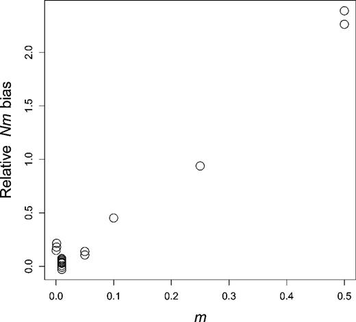
Relationship between dispersal probability and bias of estimated number of migrants for all cases in table 1.
PAC-likelihood
The PAC-likelihood approximation can easily be compared with the likelihood analysis when the latter is feasible (cases [21]–[40] in the same order as comparable strict likelihood analyses [1]–[20]). In all cases, their performance is very similar, except that PAC-likelihood estimates of the mutation rate appear unbiased or downward biased while strict likelihood ones show a slight positive bias (fig. 5). Some additional PAC-likelihood analyses were considered for lattices (cases [41]–[43]) and demonstrate good performance. Case [42] is identical to case [22] except that a larger array was considered. Expectedly, the spatial edge effects are reduced and indeed no longer apparent in this case.
![Comparison of biases by strict likelihood (all cases in table 1) and PAC-likelihood (first 20 rows of table 2). A point (case [20] by likelihood, [40] by PAC-likelihood) with huge 1/Nb bias is not shown in the last panel.](https://oup.silverchair-cdn.com/oup/backfile/Content_public/Journal/mbe/29/3/10.1093_molbev_msr262/2/m_molbiolevolmsr262f05_lw.jpeg?Expires=1716534770&Signature=L79DPu5sBFLorQ5agMuyIZk05lo~CAxCLc~bbt-GuGwRvq9SsG2v-PI~o5z0BATCKCgYs1zXPw8TigbYbuWL9oHiJJdvL6GaQSVgGVHBhFE1KiCoDEcp2JkGtcPt9WbJT4xo24IoAtW7IOJKcYw0wHpEJo0c8mCXMMieGwZzcpqSt9uPMneX1ZguWsLQ46ba6gihN3HerDag5tFFIIiaPF2bOW30adDeXpba3E-IWWzbadGygEHE2qzBLp3Z82O211W0N7OYepGDZDFgIpvQl84guPYmlDaTLaaZ0ru1hUCBu3YRyz9mQb9ucJ-~u5rYfXx5i5ERDRAo9gt-4Ar3kA__&Key-Pair-Id=APKAIE5G5CRDK6RD3PGA)
Misspecification Effects and Comparison with Moment-Based Method
In this section, we consider three sources of misspecification: the spatial binning of samples, the mutation process at marker loci, and the shape of the dispersal distribution. We also compare the performance of likelihood-based inference to a simple regression method for estimation of neighborhood in such conditions of misspecification.
The algorithms considered in this work rest on the definition of distinct demes. However, in natural populations, individuals are not clearly clustered in demes. It is tempting to analyze such populations as made of a large number of small breeding patches though there are computational limits to the number of demes that can be considered in practice. A straightforward method of clustering is according to regular spatial bins. It is therefore necessary to know how such a clustering can affect inferences. In particular, it is not necessarily obvious what are the parameter values to be estimated (the estimands) from the binned data.
For samples from a regular array, a putative estimand for Nm is the number of immigrants in each spatial bin, that is, the sum of the numbers of immigrants within each deme, reduced by the number of immigrants exchanged among demes within a bin. The estimand neighborhood size could be invariant with respect to bin size (in linear habitats, this holds provided that spatial distance is still measured in the original units not in number of bin widths). For mutation, one may assume that the estimand is the bin population size times mutation probability. In the Appendix, we show that such predictions do not always work well, in particular for Nm and g, and that the effects of binning may also depend on the distribution of samples among bins. In general, it may be difficult to make sense of Nm and g estimates.
To evaluate performance in a biologically relevant setting, we considered conditions broadly similar to those of two-dimensional analyses of the damselfly metapopulation described by Watts et al. (2007). This damselfly scenario can also serve as a basis for a realistic comparison between likelihood- and moment-based methods of inference. We have first simulated data sets with samples taken along four lines in a rotationally symmetric pattern forming the four tips of a cross. This mimics sampling along small streams in the original study. The neighborhood value and mutation rate approximate the moment and likelihood estimates from the damselfly data. An array of demes is simulated and analyzed as arrays of , , or spatial bins (table 3, cases [46]–[48]). Even by PAC-likelihood, the analysis for the larger array is computationally intensive, so the sample size considered (10 loci genotyped in 200 individuals) is smaller than in the original study. This still requires about 15 CPU days per sample on ∼2.5 GHz core processors (i.e., 7.5 CPU years in total for case [46]). The values tested by likelihood ratio are the estimands, that is, the true Nb value, and mutation probability times bin population size for .
Alternative Dispersal and Mutation Models
| Parameters | Bins | Relative Nμ | Relative 1/Nb | |||||||||
| Bias | RMSE | KS Test | Bias | RMSE | KS Test | |||||||
| 40 × 40 array, N = 50, m=0.5, g = 0.5, μ = 1 × 10⁻⁴ (Geometric distribution) | ||||||||||||
| [46] | 20 × 20 | 0.0069 | 0.15 | 0.42 | -0.036 | 0.35 | 0.19 | |||||
| [47] | 10 × 10 | 0.0054 | 0.15 | 0.39 | 0.017 | 0.42 | 0.058 | |||||
| [48] | 5 × 5 | 0.0011 | 0.14 | 0.079 | 0.14 | 0.56 | 0.00011 | |||||
| Array | N | κ | Nb | μ | (Reciprocal Poisson Gamma distribution) | |||||||
| [49] | 40 × 40 | 50 | 0.92 | 126 | 1 × 10⁻⁴ | 10 × 10 | -0.032 | 0.16 | 0.14 | 0.048 | 0.14 | 0.86 |
| [50] | 40 × 40 | 50 | 4.6 | 628 | 1 × 10⁻⁴ | 10 × 10 | -0.0073 | 0.16 | 0.32 | -0.068 | 0.27 | 0.12 |
| [51] | 40 × 40 | 50 | 23 | 3140 | 1 × 10⁻⁴ | 10 × 10 | -0.0056 | 0.15 | 0.8 | -0.46 | 0.9 | 8 × 10⁻⁴ |
| [52] | 80 × 80 | 50 | 23 | 3140 | 1 × 10⁻⁴ | 10 × 10 | 0.016 | 0.19 | 0.22 | -0.18 | 0.83 | 0.013 |
| [53] | 80 × 80 | 50 | 23 | 3140 | 1 × 10⁻⁴ | 20 × 20 | 0.015 | 0.18 | 0.21 | -0.23 | 0.79 | 0.44 |
| Stepwise mutation | ||||||||||||
| [54] | 40 × 40 | 50 | 0.92 | 126 | 1 × 10⁻⁴ | 10 × 10 | -0.54 | 0.55 | ND | 0.067 | 0.16 | 0.13 |
| [55] | 40 × 40 | 50 | 4.6 | 628 | 1 × 10⁻⁴ | 10 × 10 | -0.54 | 0.55 | ND | -0.11 | 0.34 | 0.34 |
| [56] | 80 × 80 | 50 | 23 | 3140 | 1 × 10⁻⁴ | 10 × 10 | -0.72 | 0.73 | ND | -0.4 | 0.83 | 0.56 |
| [57] | 80 × 80 | 50 | 23 | 3140 | 1 × 10⁻⁴ | 20 × 20 | -0.72 | 0.73 | ND | -0.37 | 0.79 | 0.32 |
| [58] | 80 × 80 | 50 | 23 | 3140 | 5 × 10⁻⁴ | 10 × 10 | -0.75 | 0.75 | ND | -0.28 | 0.73 | 0.4 |
| [59] | 80 × 80 | 50 | 23 | 3140 | 5 × 10⁻⁴ | 20 × 20 | -0.75 | 0.75 | ND | -0.28 | 0.69 | 0.18 |
Note.—In the 40 × 40 array, samples were taken at positions (6,20) to (10,20), and in rotationally symmetric positions (20 samples of 10 individuals in total). In the 80 × 80 array, samples were at positions (11,40) to (19,40) by steps of two, and at rotationally symmetric positions. “ND” (not done) tests means that tests would be highly significant but were not performed as they would have required estimating the likelihood of points far from the top of the likelihood surface at the detriment of computations for inference about Nb.
Effects of Binning
For binning (case [46]), estimator performance is consistent with expectations, with good coverage of the confidence intervals. The same conclusions are supported by analyses as and arrays (cases [47] and [48]). In the latter case, a distorsion of P values becomes more apparent as well as a relative bias of 0.14 for Nb. This distorsion may be in part due to the fact that many g estimates are at the boundary. This, and the high RMSE of g estimates (see case [65] in table 4, Appendix), may itself be due to the difficulty of estimating spatial effects when only a small range of distances are represented in the binned data.
Effects of Binning
| Array | Parameters or Estimands | Relative Nμ | Relative Nm | g | Relative 1/Nb | ||||||||||||
| or bins | 2Nμ | 2Nm | g | Nb | Bias | RMSE | KS Test | Bias | RMSE | KS Test | bias | RMSE | KS Test | Bias | RMSE | KS Test | |
| 10 × 10 | 0.04 | 8 | 0.5 | 100.531 | |||||||||||||
| [60] | 5 × 5 | 0.16 | 16 | 0.357 | 100.531 | -0.11 | 0.17 | 0.00063 | 0.055 | 0.45 | 5.1 × 10⁻⁷ | -0.014 | 0.35 | 8.1 × 10⁻⁸ | 0.48 | 1.22 | 4.8 × 10⁻⁸ |
| [61] | 5 × 5 | 0.16 | 8 | 0.357 | 100.531 | -0.17 | 0.23 | 1.1 × 10⁻¹⁶ | -0.17 | 0.23 | 1.1 × 10⁻¹⁰ | 0.053 | 0.21 | 0.45 | 1.34 | 1.9 | 6.4 × 10⁻¹⁵ |
| 100 | 0.4 | 20 | 0.5 | 120 | |||||||||||||
| [62] | 25 | 1.6 | 20 | 0.131 | 30 | -0.082 | 0.24 | 0.32 | 0.13 | 0.26 | 0.19 | -0.0033 | 0.13 | 0.68 | -0.015 | 0.37 | 0.71 |
| 40 × 40 | 0.01 | 50 | 0.5 | 628.319 | |||||||||||||
| [62] | 20 × 20 | 0.04 | 252.467 | 0.12791 | 628.319 | 0.0069 | 0.15 | 0.42 | 0.062 | 0.46 | 0.093 | 0.032 | 0.19 | 0.0027 | -0.036 | 0.35 | 0.19 |
| [63] | 10 × 10 | 0.16 | 297.086 | 0.083559 | 628.319 | 0.0054 | 0.15 | 0.39 | 0.014 | 0.37 | 0.32 | 0.045 | 0.24 | 1.1 × 10⁻⁶ | 0.017 | 0.42 | 0.058 |
| [64] | 5 × 5 | 0.64 | 210.365 | 0.176318 | 628.319 | 0.001 | 0.14 | 0.079 | 0.35 | 0.6 | 2.4 × 10⁻⁹ | -0.036 | 0.32 | 0 | 0.14 | 0.56 | 0.00011 |
Note.—Header lines give the three sets of true sample simulation parameters. All analyses are by PAC-likelihood. Similar results were obtained by strict likelihood for cases [60] and [62] (not shown). For easy reference, cases [63]–[65] reproduce the results for Nb and Nμ already given as cases [46]–[48] in Table 3.
Additional Effect of the Dispersal Distribution
To assess the effect of the dispersal distribution, the Poisson reciprocal Gamma distribution (Chesson and Lee 2005) is now used for the simulation of samples as described in the Methods section. Deme size was as in case [46]. Cases [49]–[51] illustrate three different values of neighborhood size, the intermediate one being as in case [46]. Good estimation of the neighborhood is achieved in all three cases (fig. 6, top, shows a typical profile likelihood surface in case [46]). However, for the largest neighborhood value the distribution of the LRT departs from ideal behavior if the spatial scale of sampling is not extended. In that case, more distant samples taken from a lattice were also simulated (case [52]).
![Examples of profile likelihood surfaces for cases [46] (top) and [57] (bottom). The surfaces are inferred from 1,024 points as described in the Appendix. In each case, the sample that yielded estimation errors closest to the RMSE values and of the same sign as the bias were selected (hence, they exhibit positive Nb estimation error since 1/Nb estimates are negatively biased, table 3). In both cases, 2Nμ=0.01; Nb=628 (top) or 3,140 (bottom). The likelihood profile surface is shown only for parameter combinations that fell within the envelope of parameter points for which likelihoods were estimated. The cross denotes the maximum.](https://oup.silverchair-cdn.com/oup/backfile/Content_public/Journal/mbe/29/3/10.1093_molbev_msr262/2/m_molbiolevolmsr262f06_ht.jpeg?Expires=1716534770&Signature=gNVhsudEuPbiIv5K1aQkTgMNZlYgINypNFLV13S3U3sfh8Mr2L0PC2f0nZz7t8WesI8OVpg9cHokIvKJtZqDUmU6y2nf0AYdZ6iKy3I28S2zlGnc0HTPtyLuUqTJBvf8f17PB5GJh9V3OY~rTzj2CTCz6aJIDZOyCFUzPY0gp0WZSq7hOsr6q5pPPPFoeuXAtTT6LLpInro6QF~fP4ByE0KIAldfwJR74~Yd7CkDDv2SaP-B4TU0UuPEpSKnAaNtrrK6FbHfaWU~fkhviJHI5V7t0MMTCIleYSJZaaWZQVYGm~NvK7XbF1tnTX6ND3OhXPaO~1FxkBPd~Jj4XnGpLw__&Key-Pair-Id=APKAIE5G5CRDK6RD3PGA)
Examples of profile likelihood surfaces for cases [46] (top) and [57] (bottom). The surfaces are inferred from 1,024 points as described in the Appendix. In each case, the sample that yielded estimation errors closest to the RMSE values and of the same sign as the bias were selected (hence, they exhibit positive Nb estimation error since Nb estimates are negatively biased, table 3). In both cases, ; (top) or 3,140 (bottom). The likelihood profile surface is shown only for parameter combinations that fell within the envelope of parameter points for which likelihoods were estimated. The cross denotes the maximum.
Additional Effect of Stepwise Mutation
Finally, the same demographic simulation conditions were also considered for markers evolving under a SMM (cases [54]–[57]). estimates are roughly halved, as previously observed for the SMM in Rousset and Leblois (2007) or even lower (case [57]; fig. 6, bottom, shows a typical profile likelihood surface in this case). Accordingly, the gene diversity is low. This implies that there may be little information for other parameters, contributing to the Nb bias and also to as many as two-third of g estimates being at the boundary (not shown). In additional simulations (cases [58] and [59]), the true mutation rate was 5-fold increased, and the number of loci increased to 20, resulting in slightly improved Nb estimation.
Comparison with Moment-Based Estimates
Alternative estimators of 1/Nb are obtained as the regression slope of estimates of pairwise to logarithm of distance (Rousset 1997) or of the pairwise statistic comparing pairs of individuals as described in Watts et al. (2007). We consider only the method below but similar results were obtained with . The 1/Nb estimators can be compared in terms of the ratio of their mean square errors and, as expected from a likelihood method, PAC-likelihood has lower error. Moreover, this discrepancy persists when alternative dispersal distributions and mutation models are considered.
For case [46], the ratio of MSEs is 0.66. Accordingly, the moment-based confidence intervals should be wider (fig. 7). However, they tend to be conservative (being often too short when the Nb estimate is small), as previously shown for this and related methods (Leblois et al. 2003, Watts et al. 2007) and accentuated by the present small sample sizes.
![Distributions of estimates and confidence intervals for Nb, by the spatial regression method and by PAC-likelihood, for case [46]. The horizontal line marks the true parameter value.](https://oup.silverchair-cdn.com/oup/backfile/Content_public/Journal/mbe/29/3/10.1093_molbev_msr262/2/m_molbiolevolmsr262f07_ht.jpeg?Expires=1716534770&Signature=nIGujiHoUemWV4qnvo-Kt6U0bm1CMIlFSfm-Eg0TeZh8tHBq9e7fVTryOxO1mAIlsNzuOV3pXbcH8cX6WB9mnJ~kiltK97LLWkfhEHC3hCaJs5PKDsS7wokxY4-pp6e-EFsL5bluWNks2-V8oF7ugVpc90g7IfSXB67K2DaC8sHIzk6BRh8pwXGZmqRI1zVkbRtpUySbKntTc99K70NPTgf0TDfNrJ05YnuAfBsNC205Or~EwM2dlODO~3-xoEZB1~4A2Uz-51I~1foMVb~HGWPFLHpaNpbMcIaCWa9jp6lMY3sqoFbnYtnnt8h~5niUP1b05l-twwClMW7TRAhpjw__&Key-Pair-Id=APKAIE5G5CRDK6RD3PGA)
Distributions of estimates and confidence intervals for Nb, by the spatial regression method and by PAC-likelihood, for case [46]. The horizontal line marks the true parameter value.
With the alternative dispersal model, the ratios are 0.27, 0.36, 0.34, and 0.46 for the four cases [49]–[52], so that the moment method appears comparatively worse for more restricted dispersal.
In case [58], where stepwise mutation is also considered, the ratio is 0.55.
According to these results, the PAC-likelihood analysis of the original damselfly data for the two-dimensional habitat should provide a more accurate and reliable estimate and confidence interval for Nb than previous moment-based analyses. Still, the results are not very different from previous estimates: 1,110 (interval 600–3,625) by PAC-likelihood (analyzed as a array) versus 753 (interval 319–3,162) by -based methods (Watts et al. 2007). They concur with the previous conclusion that the genetic estimates are only slightly higher that the demographic estimate (Nb = 555, Watts et al. 2007).
Discussion
We have presented an effective software implementation of likelihood inference under a two-dimensional model of isolation by distance and investigated the performance of inferences based on likelihood ratios in both the one- and the two-dimensional spatial models. Our results illustrate both the strengths and imperfections of such inferences: In most cases, estimators have low bias and, given the relatively small sample sizes considered, low MSE. These results are consistent with those of Rousset and Leblois (2007). When compared with a preexisting method for estimation of neighborhood, the likelihood-based estimation of neighborhood appears to be substantially more efficient and its confidence intervals to be more reliable, even when complicating factors such as the misspecification of the dispersal distribution and the binning of samples are taken into account.
However, considering the distributions of P values of LRTs underlines small but statistically detectable effects such as the small negative bias of PAC-likelihood estimates of mutation rate. Further, the assumptions inherent in the statistical model (low m, large N, and an approximate accounting of spatial edge effects) affect estimation of the Nm and g parameters. For , we found more than 2-fold relative bias in number of migrants. This could be expected from consideration of the infinite island model. In this simple case, the expected for and is , whereas the classical low-Nm approximation (for haploid N) is . The coalescent approximation fits the actual for a higher Nm value than the true one, so that Nm estimates derived from the coalescent model should be biased upward. Under isolation by distance, short-distance differentiation can be approximated by island model expectations, and we again expect, and observe, upward-biased Nm estimates. Since programs such as Migrate (Beerli and Felsenstein 1999, Beerli and Felsenstein 2001) or Lamarc (Kuhner 2006) are based on the same coalescent approximations as de Iorio and Griffiths' algorithms, the same biases should be encountered, at least when the same type of molecular markers is considered. Inference methods based on a Dirichlet distribution for allele frequencies, as follows from Wright's (1937) diffusion formula, should be affected by the same type of biases. This was observed by Faubet et al. (2007, p. 1160) when assessing the method of Wilson and Rannala (2003) on samples drawn from populations with small N and large m.
In order to better identify other possible causes of nonideal performance, we have first assumed that the dispersal distribution and the mutational process were known. We have then relaxed these assumptions and have also considered the effects of the spatial binning of samples. Both the misspecification of the dispersal distribution and spatial binning can bias the estimation of the dispersal parameters in complex ways that may render such estimates practically meaningless. However, in general neighborhood size estimation appeared robust (see also Rousset and Leblois 2007 for a linear habitat), except when the subpopulations that are binned together already exhibit a substantial fraction of the differentiation found among the most distant subpopulations. In simulations jointly considering misspecification of the dispersal distribution, of the mutation model, and the effect of a milder but realistic spatial binning, the mutation process mainly affected estimation but not Nb estimation.
The fact that neighborhood estimation appears robust implies that likelihood inference performs in the same way as a spatial regression method that would simultaneously estimate the neighborhood size from the increase in differentiation with distance (which does not rest on a coalescent approximation) and that would estimate Nm from the level of small-scale differentiation. Likelihood inference of Nb may actually be more robust than the regression method as the latter does not account for spatial edge effects. For example, in case [39] (a 10×10 array with samples taken in the corners), the regression method has an approximately 3-fold bias (details not shown), whereas the likelihood method has correct coverage.
We did not consider the effect of a so-called continuous population structure, where individuals can settle anywhere in a continuous habitat (Felsenstein 1975, Barton et al. 2002). However, in such a case, the neighborhood parameter is best defined by considering the random walk of ancestral lineages over the finite or countable positions of ancestors rather than over continuous space, so that continuous-space models can actually be understood as discrete-space models (Robledo-Arnuncio and Rousset 2010), akin to the lattice models considered in the present work. In this respect, we do not expect important differences between the estimands in the two classes of models. In both discrete- and continuous-space models, the neighborhood parameter depends on the product of an effective mean square dispersal distance and of an effective population density parameter . is defined as the asymptotic increase in mean square displacement per unit of time of a particle performing this random walk, and is defined from the asymptotic rate of encounter of ancestral lineages that each perform the same random walk and do not coalesce when they meet each other. The estimand neighborhood size defined in this way is a good predictor of the moment method performance (Robledo-Arnuncio and Rousset 2010).
A corollary of robust neighborhood estimation and nonrobust Nm estimation is that algorithms based on coalescent approximations are not most appropriate to infer the shape of the dispersal distribution. A dedicated study of inference of the shape of the dispersal distribution in a wider family of distributions would either be plagued by the effects of the coalescent approximation or should confine itself to scenarios of low dispersal probability, compared with our focal population scenarios, which would strongly restrict its usefulness.
This study has been focused on isolation by distance as it is a widespread phenomenon that has been little considered in a likelihood framework. However, this is a computationally challenging problem, and simpler problems can very easily be handled within the current software implementation. Estimation of the mutation rate parameter for a single population can be performed in seconds, and remarkably even the single locus confidence interval have practically perfect coverage in this case (not shown). Analyses under an island model are also fairly straightforward.
From the present results, likelihood inferences appear feasible in moderately sized networks of populations, and they are more efficient than moment-based method in some realistic conditions. Nevertheless, the validity of inferences is affected in complex ways by many factors and may need to be analyzed in a case-by-case basis. Further progress in algorithms and refined approximation techniques would be necessary to raise full-likelihood techniques as a general-purpose method of analysis of spatial genetic data, in particular if accurate confidence intervals are sought. This will surely encourage consideration of alternative methods to derive estimates and confidence intervals. A general alternative is the one based on simulation of summary statistics, more or less similar to currently developed ABC techniques (Beaumont et al. 2002, Marjoram and Tavaré 2006). In the latter perspective, it is worth emphasizing that coalescent approximations matter, and thus sample simulation programs based on such approximations may be misleading. More speculatively, the PAC-likelihood estimators could be considered as efficient summary statistics, though improvements in computation power and in the processing of simulated distributions will be necessary to make this a practical option.
We thank K. Belkhir, G. Dugas, A. Weisseldinger, and V. Ranwez for management and assistance in relation to the computing grids of ISEM and UFR, and J.-M. Cornuet, R. Vitalis, and two reviewers for comments on the manuscript. This is paper ISEM 2011-154. This work was supported by the Agence Nationale de la Recherche (ANR EMILE NT09-611697).
Algorithms and Implementation
Likelihood and PAC-Likelihood Computation
The likelihood for individual parameter points is estimated as the average value of a statistic over independent realizations of possible ancestral histories of a sample, which distribution is generated by an absorbing Markov chain with the allelic state in the common ancestor as the absorbing state (e.g., Griffiths and Tavaré 1994, de Iorio and Griffiths 2004a, de Iorio and Griffiths 2004b). In particular, the likelihood computations rest on the computation of de Iorio and Griffiths' terms, which are approximations for the probability π that an additional gene sampled from a population is of a given allelic type, conditional on the allelic counts of a previous sample. The s may be viewed as biased estimates of the πs, and importance sampling techniques, where the s also affect the distribution of realizations of the Markov chain, are used to obtain an unbiased estimate of the likelihood (see de Iorio and Griffiths 2004b for a more detailed description).
This algorithm differs from those based on long runs of a recurrent Markov chain, which is the better known Markov Chain Monte Carlo type of algorithms considered in Migrate (Beerli and Felsenstein 1999, Beerli and Felsenstein 2001, Lamarc (Kuhner 2006) or in the IM suite of programs (Hey and Nielsen 2004, Hey 2010). Therefore, the lingering issue of assessing the convergence of a recurrent Markov chain does not arise. On the other hand, the estimator of likelihood may not be consistent for certain choices of the absorbing Markov chain (Stephens and Donnelly 2000), but this problem is not apparent in the present work.
An elementary modification of the likelihood estimation algorithm, which however saves a substantial fraction of computation time, is to perform the final likelihood computation when the ancestral history reaches the two-lineages states by using standard formulas for identity in state in migration matrix models, taken in the coalescent limit (e.g., de Iorio et al. 2005) rather than by the Markov chain method. This was implemented here.
The average computational burden for each ancestral history increases with the number of events (mutation, migration, coalescence) in each history and with the amount of computation for each event. Both increase with the number of demes. The s can be obtained as the solution of a linear system , where each dimension of the A matrix is the number of subpopulations. In large arrays of demes, the computation time of this step can be reduced by using an iterative method (preconditioned conjugate gradient algorithm) for solving the linear system, provided approximate initial values are easy to compute. For linear habitats, the solution of the system defined by a pentadiagonal subset of elements of A was used as the starting point (Rousset and Leblois 2007). In two-dimensional habitats, the solution for the A matrix for the island model (, other parameters unchanged) is used as a starting point as it can be efficiently computed using the Sherman–Morrison formula (Bartlett 1951).
Although networks of more that 100 populations were considered in this study, one CPU year or more may be necessary to analyze a typical sample in this context. Because the estimation of likelihood in different parameter points proceeds independently, such an analysis can easily be performed in a much shorter time on a computer grid. Still, it is unpractical to analyze hundreds of samples in such conditions. A fast alternative in such cases is the PAC-likelihood method. In the incarnation previously described in Cornuet and Beaumont (2007) and Rousset and Leblois (2007), PAC-likelihood uses de Iorio and Griffiths' as estimates for the corresponding π, without any recourse to the importance sampling methodology to correct for any resulting bias. The computation time of PAC-likelihood increases more slowly with the number of demes because it is independent of the number of possible events in the history of the sample. In particular, for fixed number of demes, the differences in computation time between likelihood and PAC-likelihood estimation increases when a large number of migration events occur in the realized ancestral histories that is when Nm increases. Rousset and Leblois (2007) found that PAC-likelihood could by 500 to 1,000 times faster than likelihood, but the difference can be larger depending on Nm values. In many of the simulations of table 3, parameter points with Nm values of 500 or more had to be considered, and only PAC-likelihood computation was feasible for such points.
Likelihood Surface Estimation
Smoothing of Likelihood Estimates.
A likelihood surface is inferred from likelihood estimates in different points. The smoothing technique known as Kriging (e.g., Cressie 1993, Zimmerman and Stein 2010) was used in de Iorio et al. (2005) and Rousset and Leblois (2007) for that purpose and is still used in this paper. However, compared to previous works, the implementation of Kriging had to be optimized in order to yield good confidence intervals. The Kriging predictor function depends on covariances between response values at different distances in parameter (predictor variables) space, and these covariances are described by a covariance family and some covariance parameters.
The covariance parameters are now estimated by so-called generalized cross-validation (Golub et al. 1979), using the Matérn covariance family, which includes a smoothness parameter ν. In general, the estimated ν was the maximum allowed value (i.e., 4) in our estimation procedure, which generates smooth likelihood surfaces, as expected. In cases [52]–[59] (table 3), a high minimal allowed value () had to be imposed to obtain consistently good results. However, it is always wise to begin with less constrained ν estimation, as this might reveal problems with the points subject to smoothing.
We do not present specific checks of the accuracy of the smoothing step here, as in the end what matters are the properties of confidence intervals. When these had poor properties, it was repeatedly checked that the Kriging steps were not the cause of concern by increasing the density of likelihood points considered. Failure of Kriging can also easily be detected on individual data sets from a diagnostic plot of the residual errors of prediction, provided by the program.
All algorithms used for Kriging and cross-validation are described in Nychka (2000) and implemented in the fields package (Fields Development Team 2006) of the R statistical software (R Development Core Team 2004). However, numerical issues related to the inversion of nearly singular matrices led us to independently reimplement these algorithms. A C++ library interfaced with R is distributed along our main software to perform Kriging. Likelihood surface prediction may be very poor when extrapolation is made out of the range of parameter values of Kriged points. For this reason, the predictor was only applied to parameter points within the convex envelope of the Kriged points. Convex envelope computations were performed using the rcdd package (Geyer and Meeden 2008). All the analyses described in this study (estimation of likelihood in individual points by de Iorio and Griffiths' algorithms, Kriging, graphical output of likelihood and profile likelihood surfaces as shown in figs. 2 and 6) can be performed with the Migraine software, a C++ executable, without knowledge of Kriging nor of the R language. Migraine is free open source software. Its current distribution page is http://kimura.univ-montp2.fr/∼rousset/Migraine.htm. Multiple parameter tests are implemented in this software but not further discussed here.
Computation Settings
The settings described in this section apply to all simulations unless mentioned otherwise.
Exploration of Parameter Space.
Final likelihoods are estimated from 1,024 points, obtained in two steps. In the first step, 512 parameter points are sampled uniformly. For samples simulated under the geometric dispersal model, the initial range of parameter values explored is one-third to three times the parameter value for and Nm and 0–0.999 for g. For samples simulated under a SMM, the initial bounds were further halved. For samples simulated under the Poisson reciprocal gamma dispersal model, the initial range was one-third to three times Nb/π (which coincides with the initial range under the geometric model when ).
Likelihoods are estimated for the first 512 points, and for one every 30 of them, a second replicate estimate is computed. A likelihood surface is inferred from these likelihoods by Kriging (including a cross-validation step), and a convex envelope putatively including the whole confidence region (and possibly extending beyond the original parameter ranges) is constructed. The parameter space in which the convex envelope is defined is the same as for Kriging. Another envelope extending z times as far from the barycenter of the original envelope is defined for given z. In most simulations, 512 additional points were sampled approximately uniformly within the extended envelope with . In the latest simulations (in particular, cases [52]–[59]), a slightly more involved procedure was used, where half of the points are sampled uniformly within the envelope with and the other half in the envelope with . Either way, these procedures appears very efficient in that most of the points sampled in this way are indeed on the “top” of the likelihood surface and contribute to the computation of final likelihood ratio tests and confidence regions.
In the second step, the likelihood for the 512 additional points are estimated, with again replicates for one every 30 of them, and a likelihood surface is inferred by Kriging from all 1,024 points (including a new cross-validation step). The effect of additional points from a third iteration was repeatedly checked and found to have no impact on the conclusions.
Other Settings.
In most cases, for each locus and each parameter point, the likelihood estimate is obtained from 30 replicates of the absorbing Markov chain (i.e., 30 possible ancestral histories) or 30 replicates of the PAC-likelihood algorithm. In cases [52]–[59], only five replicates of the IS or PAC-likelihood algorithms were computed for each locus and each parameter point, as preliminary simulations suggested that this was sufficient.
Specific Settings for Large g.
If the true g value is 0.99999, uniform sampling of hundreds of g values is unlikely to generate g values large enough, so that ultimately no predicted likelihood value will be available for the true g value or for the true neighborhood value. Various ad hoc corrections of the sampling of parameter points could be considered. Here, we performed uniform sampling of rather than g. Kriging was performed on the same variable. This parameterization could be more generally useful when there is a plateau of high likelihood values for large values of the neighborhood size, which is expected for samples simulated under high neighborhood values.
Comparison with Moment-Based Inferences.
Likelihood-based inferences of neighborhood size were compared with moment-based ones (e.g., Rousset 1997, Vekemans and Hardy 2004, Watts et al. 2007) as implemented in the software Genepop, version 4.1 (Rousset 2008), wherein confidence intervals are constructed by the ABC bootstrap method (DiCiccio and Efron 1996).
Misspecification Effects Due to theCoalescent Approximation
Samples are simulated under an exact backward generation-by-generation algorithm, where no “large N” approximation is used. Deme size N, forward migration probabilities, and mutation probability u are all distinct parameters, whereas the estimation algorithm is based on limit results for large N, small backward immigration probabilities, and small u. In the sample simulation program, edge effects can be accounted for in a simple mechanistic way by computing the backward dispersal distribution in a focal deme as the relative forward migration probabilities from every deme (including the nonimmigration probability from the focal deme itself), where the forward probabilities are identical from any deme. But this cannot be done in the estimation algorithm, as the coalescent model does not depend on the nonimmigration probability but only of number of immigrants (product of deme size and immigration probabilities) from other demes. To put it another way, in the coalescent limit, the forward nonmigration rate is the limit value of as and ; this is infinitely larger than any immigration rate from other demes and cannot be used to define a backward probability distribution.
This means that the statistical model is intrinsically misspecified when applied to samples generated by the exact backward algorithm. One way to overcome this discrepancy is to simulate samples under coalescent assumptions, and this case has been considered. However, an extended assessment of performance under such conditions would not give any idea of the implications of misspecification for analyses of data from populations where dispersal probabilities are not vanishingly low. Therefore, we more generally controlled the number of immigrants according to the rules described in the main text.
Effects of Binning
A good understanding of the effects of binning on inferences is obtained when a rule is given to generate estimands that are shown to be estimated with low bias and ideally good coverage of confidence intervals. For example, bin population size times mutation probability is a good estimand as the estimates have low bias relative to this value. Departures from this rule in the simulations can be attributed to the PAC-likelihood bias rather than to binning per se. However, for the dispersal parameters, no rule was found that correctly predicts all estimands in all cases investigated. For example, the expected number of immigrants in a bin is not always the correct Nm estimand. Nevertheless, we can deduce estimands for binned data from the estimands of the moment-based regression method: the estimand Nm is deduced from the inferred between the nearest bins, and this appears to work well. Indeed, this may not only account for the effects of binning but also for deviations from the large N, low m approximation. Likewise, the Nb estimand can be deduced from the increase of differentiation with distance in the binned data, and the g estimand can then be deduced from Nm and Nb.
However, there are several drawbacks with these predictions. First, they can be derived from simple analytical arguments in some cases, but must otherwise be generated by a regression analysis of binned data with a large number of loci and are not uniquely related to the true parameter values only but may also depend on the sampling design as shown below. Second, the Nb estimand derived from the slope of the regression may not be a valid prediction in conditions where the regression method is expected to poorly estimate Nb. For example, the regression method does not account for edge effects in contrast to the likelihood method. Peripheral demes receive fewer immigrants and thus are more differentiated than central demes, which biases regression Nb estimates downward when samples are taken from peripheral demes. In fact, it is both more easily interpretable and overall a more accurate prediction to assume that the estimand Nb is the true Nb value. The following examples illustrate these conclusions.
Under an island model, different results are expected whether only populations are binned or whether samples are binned too. As an illustration of the first case, consider an array of populations binned into a array, but samples come from nonadjacent populations and therefore go into different bins. A standard analysis of the binned data will yield the same and Nm estimates as that of the original data because the binned samples are indistinguishable from the original samples, and estimation per se does not use any extra information. By contrast, when (say) pairs of samples are binned too, the estimates are halved, so that Nm estimates are roughly plus twice the original value. As an illustration, we reconsidered the simulation conditions of case [39] (, , and in a two-dimensional habitat). For bins covering two lattice units, wherein pairs of samples are binned, the estimand is (or more exactly 16.5) according to the island model argument, and then from equation (1), . By contrast, if four of the eight sampled populations are taken at position (3,3) and rotationally symmetrical positions rather than at position (2,2) and rotationally symmetric positions, samples are no longer binned when populations are binned. Simulations conditions are otherwise identical to the previous ones, but the estimand is . Simulation results (case [60] vs. [61]) confirm this predicted contrast. For Nb, if true values are taken as the estimands, estimation is poor as shown in the table. However, performance is also poor when estimands are deduced from the regression analysis (not shown). In this case, regression estimates are affected by edge effects, as samples come from peripheral demes even in the absence of binning.
This example shows that the effects of binning may be difficult to predict as they are affected by the sampling design, and all the more so as in real data analyses, different number of samples may fall in different bins. The following simulations and all those reported in table 3 incorporate the latter feature.
For the simulation conditions of case [44] (m=0.025, , , and Nb in a linear habitat), a regression analysis of a 2,000-loci data set shows that the fitted differentiation between adjacent bins of four demes is only slightly lower than that between adjacent demes (estimated vs. 0.040). The slope of the regression against geographical distance (in bin width units) is roughly 4-fold increased, which is indeed expected from the mere effect of the change of spatial scale (equivalently, the Nb estimand is invariant if distance is always measured in the same spatial units). For simplicity, in the analysis of likelihood performance, we assumed that the Nm estimand was unchanged by binning (thereby expecting a small positive bias) and that Nb estimand is the true Nb value, only 4-fold reduced by the change of scale. All these predictions are well supported (case [62]).
A similar analysis was conducted in conditions closer to the damselfly example. Estimands were deduced from a regression analysis of a 2,000-loci data set for three binning levels. The estimand Nb inferred in these three cases deviated at most by 43% from the true value (in particular, in two dimensions, the regression is relative to logarithm of distance and a change of spatial scale has no effect on the regression slope). On the other hand, there was an almost 6-fold variation of the Nm estimands from the true Nm value (up to 297 vs. 50, as shown on the left of table 4). As above, in the analysis of likelihood performance, we varied the Nm estimand as given by the regression analysis but fixed the Nb estimand to the true value as shown in the table.
The predictions are again well supported (cases [63]–[65]), although some distorsion of P values is observed for g (maybe because many estimates are at the boundary) and becomes evident for the other dispersal parameters under the highest level of binning.
These results show that the effects of binning on likelihood inferences of dispersal parameters are largely predictable from its effect on spatial regression analyses when the latter are meaningful. However, the effects on Nm and g are complex. In the main text, we consider only Nb and estimates, where Nb estimands are taken to be the true values.
References
Author notes
Associate editor: Noah Rosenberg
