


Abstract
We analyse the clustering of the Sloan Digital Sky Survey IV extended Baryon Oscillation Spectroscopic Survey Data Release 14 quasar sample (DR14Q). We measure the redshift space distortions using the power-spectrum monopole, quadrupole, and hexadecapole inferred from 148 659 quasars between redshifts 0.8 and 2.2, covering a total sky footprint of 2112.9 deg2. We constrain the logarithmic growth of structure times the amplitude of dark matter density fluctuations, fσ8, and the Alcock–Paczynski dilation scales that allow constraints to be placed on the angular diameter distance DA(z) and the Hubble H(z) parameter. At the effective redshift of zeff = 1.52, fσ8(zeff) = 0.420 ± 0.076, |$H(z_{\rm eff})=[162\pm 12]\, (r_s^{\rm fid}/r_s)\,{\rm km\, s}^{-1}\,{\rm Mpc}^{-1}$|, and |$D_A(z_{\rm eff})=[1.85\pm 0.11]\times 10^3\,(r_s/r_s^{\rm fid})\,{\rm Mpc}$|, where rs is the comoving sound horizon at the baryon drag epoch and the superscript ‘fid’ stands for its fiducial value. The errors take into account the full error budget, including systematics and statistical contributions. These results are in full agreement with the current Λ-Cold Dark Matter cosmological model inferred from Planck measurements. Finally, we compare our measurements with other eBOSS companion papers and find excellent agreement, demonstrating the consistency and complementarity of the different methods used for analysing the data.
1 INTRODUCTION
The large-scale structure of the Universe encodes a significant amount of information on how the late-time Universe has evolved since the accelerated expansion became the dominant component of the cosmos at z ≲ 2. One way to access this information is through spectroscopic observations of dark matter tracers, such as galaxies, quasars, or inter-galactic gas. Measuring the correlation function of these tracers allows to infer the distribution of dark matter of the Universe and to constrain cosmological parameters such as the matter density of the Universe, namely Ωm, how gravity behaves at large scales, or to put constraints in the total neutrino masses and its effective number of species.
Two complementary approaches to extract such information are the baryon acoustic oscillations (BAOs) and redshift space distortions (RSDs). The BAO technique measures the BAO peak position of the observed tracer to infer the evolution of the Universe since the epoch of recombination, when the BAO peak was imprinted in the matter distribution. The BAO signal was detected on the galaxy distribution for the first time in the Sloan Digital Sky Survey (SDSS; Eisenstein et al. 2005) and in the 2-degree Field Galaxy Redshift Survey (2dFGRS; Cole et al. 2005a). The RSD technique (Kaiser 1987) examines the information of the radial component of the peculiar velocity field and the corresponding distortion in the position of tracers in redshift space. Such distortions contain information about how gravity behaves at intercluster scales (|${\gtrsim }10\ \rm {Mpc}$|) as well as the total matter content of the Universe. Since the distortions caused by the peculiar velocity field are coherent with the growth of structure, the RSD technique is sensitive to the matter content and to the model of gravity of the Universe.
The extended-Baryon Oscillation Spectroscopic Survey (eBOSS; Dawson et al. 2016), part of the SDSS-IV experiment (Blanton et al. 2017), has been constructed, in part, to measure redshifts for approximately 500 000 quasars at 0.8 < z < 2.2 (Myers et al. 2015, including spectroscopically confirmed quasars previously observed in the SDSS-I/II/III). Compared to previous SDSS large-scale projects, the eBOSS quasar sample presents relatively low number density of objects, which for the current data release 14 (DR14; Abolfathi et al. 2017), oscillates typically between 1 × and 2 × 10⁻⁵ [Mpc/h]3. However, eBOSS will compensate for this drawback by covering a large volume of the Universe in a redshift range, which has been barely unexplored to date by any spectroscopic survey.
The selection of quasars in eBOSS uses two different techniques: (i) a ‘CORE’ sample uses a Bayesian technique called XDQSOz (Bovy et al. 2012) that selects from the SDSS optical ugriz imaging combined with mid-IR imaging from the Wide-Field Infrared Survey Explorer (WISE) satellite; and (ii) a selection based on variability in the multi-epoch imaging from the Palomar Transient Factory (e.g. Palanque-Delabrouille et al. 2016). A full description of these selection techniques is presented in Myers et al. (2015), alongside the characterization of the final quasar sample, as determined by the early data. These early data were observed as a part of SEQUELS (Sloan Extended QUasars, ELG and LRG survey), part of SDSS-III and -IV, which acted as a pilot survey for eBOSS (Dawson et al. 2013; Ross et al. 2012a).
Recently, Ata et al. (2018) measured the isotropic BAO scale using the same DR14 quasar sample (DR14Q). In the present paper we describe a complementary analysis based on RSD which extends the anisotropic signal to the previous BAO analysis. In particular, we measure the power-spectrum monopole, quadrupole, and hexadecapole from the DR14Q sample in the redshift range 0.8 < z < 2.2. Pioneering works such as Blake et al. (2011) and Rota et al. (2017) have also studied the clustering of galaxies at high redshift using the power-spectrum statistics on the WiggleZ1 and VIPERS2 samples, respectively. We perform the following complementary analyses: (i) we examine the whole redshift bin and perform the measurement of parameters of cosmological interest at the effective redshift, zeff = 1.52; (ii) we explore the cosmological constraints by setting the ratio of parameters α∥/α⊥ to be 1 (see equations 16 and 17 for definitions) or to leave them as free parameters; (iii) we use three different redshift estimates, based on different features of the quasar spectra; and (iv) we separate the full redshift range in three overlapping redshifts bins, lowz between 0.8 ≤ z ≤ 1.5; mid-z between 1.2 ≤ z ≤ 1.8 and high-z between 1.5 ≤ z ≤ 2.2, and measure cosmological parameters in each of these three redshift bins, where the correlation among the parameters at different redshift bins is also computed. In all cases, we focus on measuring the logarithmic growth of structure times the amplitude of dark matter density fluctuations, fσ8(z). For those analyses where α∥ and α⊥ are treated as free independent parameters, we also measure the angular diameter distance, DA(z), and Hubble parameter, H(z).
This paper is structured as follows. In Section 2, we describe the data set used in the paper, including how the actual quasars have been targeted, their redshifts estimated, and also the techniques to produce the quasar mocks used in this paper. In Section 3, we present the methodology of our analysis, how the power-spectrum multipoles have been measured, and the theoretical model used for measuring the cosmological parameters. In Section 4, we present the power-spectrum multipoles measurements and how they compare to the mocks and to the best-fitting models. In Section 5, we perform systematic and robustness tests, using mocks and N-body simulations, in order to evaluate the systematic error budget. Section 6 displays the final results in terms of cosmological parameters measured from the quasar sample using the analyses described above, and Section 7 displays the cosmological implications of our findings. This paper is presented alongside several companion papers that perform complementary and supporting analyses on the same DR14Q sample. Hou et al. (2018) and Zarrouk et al. (2018) perform a reciprocal RSD analysis to the one presented in this paper, but in configuration space instead of Fourier space. Zhao et al. (2018) and Ruggeri et al. (2018) perform RSD analyses using a redshift weighting technique, which accounts for a redshift evolution of the cosmological parameters across the considered redshift bin. A more detailed description of these works, along with a comparison on the predicted cosmological parameters, is presented in Section 8. Finally, in Section 9, we present the conclusions of this paper.
2 DATASET
We start by describing the DR14Q data set features in detail, along with the mock catalogues used in this work.
2.1 SDSS IV DR14 quasar sample
We review the imaging data that have been used to define the observed quasar sample, which is later selected for spectroscopic observation, how the spectroscopy for each quasar target is obtained, and how the quasar redshifts are measured.
All the eBOSS quasar targets selected for the DR14Q catalogue (Pâris et al. 2018) are based on the imaging from SDSS-I/II/III and the WISE (Wright et al. 2010). We briefly describe these data sets below. SDSS-I/II catalogues (York et al. 2000) imaged a 7606 deg2 northern and 600 deg2 southern parts of the sky in the ugriz photometric pass bands (Fukugita et al. 1996; Smith et al. 2002; Doi et al. 2010) and were released as part of the SDSS DR7 (Abazajian et al. 2009). The SDSS-III catalogues (Eisenstein et al. 2011) observed additional photometry in the SGC area, increasing the contiguous footprint up to 3172 deg2, and were released as part of DR8 (Aihara et al. 2011). Further astrometry improvement of these data was presented in DR9 (Ahn et al. 2012). All the photometric data were collected on the 2.5-metre Sloan Telescope (Gunn et al. 2006), located at the Apache Point Observatory in New Mexico in the USA, using a drift-scanning mosaic CCD camera (Gunn et al. 1998). The eBOSS project does not add any extra imaging area to that released in DR8, although it takes advantages of upgraded photometric calibrations of these data, so-called ‘uber-calibration’ (Padmanabhan et al. 2008; Schlafly et al. 2012), released under the name of SDSS DR13 (Albareti et al. 2017). In addition, the WISE satellite (Wright et al. 2010) observed the full sky using four infrared channels centred at |$3.4\, \mu {\rm m}$| (W1), |$4.6\, \mu {\rm m}$| (W2), |$12 \, \mu {\rm m}$| (W3), and |$22 \, \mu {\rm m}$| (W4), and the eBOSS quasar sample makes use of W1 and W2 band for its targeting.
The quasar target selection criteria for eBOSS is presented in Myers et al. (2015). Objects that fulfill this criteria and without any previously known and secure redshift measurements are flagged as ‘QSO EBOSS CORE’ selected for spectroscopic observation and assigned an optical fibre. The spectroscopic observation are performed using the BOSS double-armed spectrographs (Smee et al. 2013), which cover the wavelength range of 3600 ≤ λ[Å] ≤ 10 000, with R = 1500 up to 2600. The description on how the pipelines process the data from a CCD level to a 1D spectrum level, and eventually to the measurement of the redshift are described in Albareti et al. (2017) and Bolton et al. (2012). The sources of redshifts are divided into three classes: (i) Legacy, where the quasar redshifts are obtained by SDSS I/II/III via non-eBOSS-related programmes; (ii) SEQUELS, where the redshifts are obtained from the Sloan Extended QUasar, ELG and LRG programme (SEQUELS; Pâris et al. 2017); and (iii) eBOSS, for those previously unknown quasar redshifts obtained by the eBOSS project. The eBOSS quasar redshifts represent more than 75 per cent of the redshifts in the current DR14Q catalogue. For further details on the imaging data, target selection criteria and the final construction of the DR14Q catalogues we refer the reader to Pâris et al. (2018).
2.1.1 Redshift measurements
One of the main challenges of using quasars as dark matter tracers is the reliability of their spectral classification and consequently their redshift estimation. Although the typical quasar spectrum has wide and prominent emission lines, the existence of quasars outflows may produce systematic shifts in the location of the broad emission lines, which may lead to uncorrected errors in the measurements of their redshifts (Shen et al. 2016). Therefore, having an accurate measurement of quasar redshift is key for achieving the scientific goals of SDSS-IV/eBOSS. For the present DR14Q catalogue, we use a number of different redshift estimates to test the impact of these potential systematics in the final scientific outcome.
The large number of quasar targets in the current DR14Q catalogue makes the systematic visually inspection procedure (used in the previous SDSSIII/BOSS Ly α analyses) unfeasible. However, the observations taken on the subprogramme SEQUELS were all visual inspected, which tested the performance of the automated classification used in the whole DR14Q. The automated pipeline was able to securely classify 91 per cent of the quasar spectra targeted for clustering studies; less than 0.5 per cent of these classifications were found to be false when visually examined (Dawson et al. 2016). Among the remaining 9 per cent of objects, which the automated pipeline failed to report a secure classification, approximately half were identified as quasars when they were visually inspected. As described in Pâris et al. (2018), the DR14Q combines automated pipeline together with visual inspections results, providing a variety of value-added information, containing three automated redshift estimates that we consider in this paper – zPL, zPCA, and |$z_\rm {{Mg}\,}{\rm {\small II}}$|.
The zPL automated classification uses a Principle Component Analysis (PCA) decomposition of galaxy and quasar templates (Bolton et al. 2012), alongside a library of stellar templates, to fit a linear combination of four eigenspectra to each observed spectrum. The reference sample for these redshift estimates are visually inspected quasars from SEQUELS.
The zPCA automated classification uses a PCA decomposition of a sample of quasars with redshifts measurements at the location of the maximum of the Mg ii emission line, fitting a linear combination of four eigenvectors to each spectrum. In addition, this classification accounts for the potential presence of absorption lines, including broad ones, and it is trained to ignore them.
The |$z_{\rm Mg\, {\small II}}$| automated classification uses the maximum of the Mg ii emission line at 2799 Å. This broad emission line is in principle less susceptible to the systematic shifts produced by astrophysical phenomena; when a robust measurement of this line is present, it offers a minimally biased estimate of the systemic redshift of the quasar. Consequently, this method produces an extremely low number of redshift failures (less than 0.5 per cent). On the other hand, this method is more susceptible to variations in the signal-to-noise ratio. When this emission line is not detected in the spectrum of the quasar, the |$z_{\rm Mg\, {\small II}}$| automated classification uses the zPL prescription.
A comparison of the performance of these redshift estimates is presented in table 4 of Pâris et al. (2018) along with visually inspected redshifts. For the DR14Q, we adopt as a standard redshift estimate zfid, which consist of any of the three options described above depending on the particular object (see Pâris et al. 2018 for further details), which provides the lowest rate of catastrophic failures. In order to test the robustness of the different redshift estimates, we run at the same time our science pipeline code on the DR14Q using zfid, zPCA, and |$z_{\rm Mg\, {\small II}}$|, as we did for the BAO analysis in Ata et al. (2018).
2.1.2 DR14Q catalogue details
The DR14Q catalogue used in this paper (Pâris et al. 2018) comprises 158 757 objects between 0.8 ≤ z ≤ 2.2 that the automatic pipeline has classified as quasars. 20 641 of these objects were also visually inspected and confirmed to be quasars and their redshifts were also determined. 148 659 of these quasars have a secure spectroscopic redshift determination and are the objects used in this paper. The remaining objects 10 098, either did not received a spectroscopic fibre or the redshift could not be determined accurately, as we describe below in more detail.
5188 objects were photometrically identified as potential quasars, but did not receive a spectroscopic observation. The fibre allocation is designed to maximize the number of fibres placed on targets, considering the constraints of the physical size of the fibres, which correspond to an angle in the focal plane of 62 arcsec, which at z = 1.5 corresponds to 0.54 Mpc. The fibre-assignment algorithm is therefore sensitive to the target density of the sky, so highly populated regions tend to be covered by several tiles. This overlap of tiles locally resolves some collision (1015 quasars redshifts are identified at less than 62 arcsec angular separation, 677 in the northern Galactic hemisphere and 338 in the southern). In Section 2.2, we describe how the unobserved quasar due to fibre collisions are treated.
4910 objects were securely classified by the automated pipeline as quasars, but their redshifts could not be securely determined and did not receive a visual inspection. The distribution of these objects is not uniform across the plate position. We refer to these objects as ‘redshift failure quasars.’ In Section 2.2, we describe how we treat these objects in our analysis. Fig. 1 displays the success rate of securely measuring the redshift of a quasar (number of successfully identified redshifts over total number of objects) as a function of the fibre location in the plate. For each tile in the survey, the vertical axis is aligned to lines of constant declination. The top panels show the success rate produced by the automated pipeline (without any visual inspection), whereas the bottom panels display the success rate after a fraction of the objects were visually inspected. The non-uniform distribution of failure rates across the plate is produced by the non-uniform efficiency of the detectors that record the spectra. The fibres positioned on holes on the left and right edges of the plate are most frequently fibres on the edges of the fibre slit in the spectrographs, corresponding to edges of the spectrograph camera focal plane for which the optical aberrations are larger. The variation of the sensitivity of the spectrograph across its position can reach 5 per cent (Laurent et al. 2017).
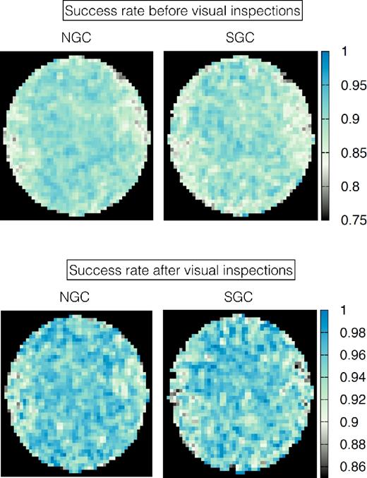
Redshift success rate as a function of plate position for the DR14Q catalogue after and before visual inspections, top and bottom panels, respectively. The higher failure rate (lower success rate) in the edges of the plate across the x-axis is caused by the less sensitive areas of the detector associated with those plate regions. The higher failure rate in the SGC plates is associated with a poorer photometric conditions in the SGC compared to those in the NGC. For each tile of the survey, the x-axis of the plate is aligned along the iso-declination lines, and the y-axis along the iso-right ascension lines, in such a way that the top areas of the plate in the figure correspond to objects with higher declination than the lower areas of the plate.
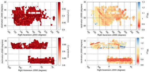
The observed objects are distributed along an angular footprint (see Fig. 3) with an effective area of 2112.9 deg2, with three disconnected regions: 1 in the Northern Galactic Cap (NGC) whose effective area is 1214.6 deg2, and two in the Southern Galactic Cap (SGC), with a total area of 898.3 deg2. The sub-region of the SGC with declinations <10 deg has an area of 412.2 deg2, and the other one has an area of 486.1 deg2.
In total, the DR14Q sample contains an effective volume3 of 0.246 Gpc3 that corresponds to an associated comoving volume of ∼32 Gpc3. The large difference between these two volumes is caused by the factor |$\lbrace P_0\bar{n}(r)/[1+P_0\bar{n}(r)]\rbrace ^2$| in the effective volume definition. In case we had a high density number of objects, |$P_0\bar{n}\gg 1$|, both effective and comoving volume would be similar, as |$\lbrace P_0\bar{n}(r)/[1+P_0\bar{n}(r)]\rbrace ^2\rightarrow 1$|. On the other hand, for the DR14Q sample we have P0 ∼ 6 × 10³ [h−1 Mpc]3 and |$\bar{n}\sim 10^{-5}\,[h\,{\rm Mpc}^{-1}]^3$|, and therefore, |$P_0\bar{n}\ll 1$|, indicating that we are in a shot noise dominated regime and the two definitions are substantially different. The effective volume should be interpreted as the fraction of the associated comoving volume utilized for measuring the power at the wavenumber whose P(k) is P0. Therefore in terms of Fisher information, the covariance matrices scale according the effective volume.
All quoted distances in this work correspond to comoving and all quoted volumes are effective volumes according to Tegmark (1997) unless mentioned otherwise.
2.2 Weights
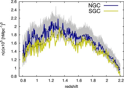
Mean density of 148 659 quasars in the DR14Q catalogue as a function of redshift, for the NGC and SGC regions in blue and yellow lines, respectively. The slight difference between the two regions is caused by differences in the target efficiency. The black dashed lines correspond to the adopted smoothed model for producing the mock catalogues. In grey, we have overplotted the mean density of 100 ez-mock realizations with the NGC selection function, which shows and excellent agreement with the data.
2.2.1 Spectroscopic weights
The spectroscopic completeness is mainly affected by two effects, the fibre collisions, and redshift failures. We have briefly described these processes above.
The physical size of the optical fibres prevents the observation of two quasars at an angular scale lower than 62 arcsec angular separation using a single tile. This effect is partially mitigated by overlapping tiles in those regions of the sky, where the concentration of targets is high. However, we still miss a small fraction of quasars due to this effect. We account for this effect by up-weighting the lost target to the nearest neighbour with a valid redshift and spectroscopic classification (always within 62 arcsec unless it has been flagged as a redshift failure). This weight is denoted as wcp, which is 1 by default for all those quasars that have not been up-weighted, and an integer >1 for the cases of fibre collisions. In total, 4 per cent and 3 per cent of the eBOSS quasar targets are flagged as fibre close pairs in the NGC and SGC, respectively. A fraction of these up-weighted quasars are true companions of the lost target in physical distance. In these cases, the up-weight is physically motivated: we displace the lost target by a small cosmological distance (few Mpc) along the line of sight (LOS), which barely distorts the clustering signal. However, for the cases where two targets are not true companions, and the LOS projected distance is large (hundreds of Mpc), moving targets along the LOS does produce a spurious clustering signal along the LOS with respect to the clustering across the LOS. More complex prescriptions based on the probability distribution of the close-pairs along the LOS have been recently presented in the literature (Bianchi & Percival 2017; Hahn et al. 2017). In this work, we do not implement these techniques, which may have a subdominant contribution with respect to the statistical errors, and leave their implementation for future data releases.
We have shown above that the efficiency in which the redshift of a quasar is inferred depends on its position in the plate. In previous data releases of the BOSS survey, the fraction of objects that were classified as redshift failures was less than |$1\hbox{ per cent}$|. For the DR14Q, the percentage of failures has increased up to 3.4 per cent and 3.6 per cent in the NGC and SGC, respectively, due to the more challenging task of measuring the redshift of a quasar at z ≃ 1.5, compared to, e.g., an LRG at z ≃ 0.5. In the recent BAO analysis of the DR14Q data (Ata et al. 2018), we opted to correct the redshift failures with a similar procedure as the one used to correct for fibre collisions: up-weighting the lost target to the nearest neighbour with a valid redshift and spectroscopic classification, what we designate wnoz. However, later we will show that this prescription produces a spurious signal in the LOS-dependent quantities, such as the quadrupole and hexadecapole, which are later transmitted to systematic shifts on the fσ8 value.
2.2.2 Imaging weights
We make use of the imaging weights defined in Laurent et al. (2017) and applied to the DR14Q catalogues in Ata et al. (2018). These weights are required in order to remove the spurious dependency on the 5σ depth magnitude, known as ‘depth’, and Galactic extinction. Laurent et al. (2017) found that quasars are more securely identified where the value of the depth larger, and Galactic extinction is the variable that most affects differences in depth among the SDSS imaging bands, as they were almost simultaneously observed. The most important observational systematics identified in Laurent et al. (2017) were those related to the depth in the g-band magnitude and Galactic extinction, which used the map determined by Schlegel, Finkbeiner & Davis (1998).
2.2.3 Targeting completeness and veto mask
We apply a veto mask to the DR14Q catalogue in order to exclude sectors in potentially problematic regions. For the DR14Q catalogues, we veto areas under the same conditions than those in BOSS DR12 (Reid et al. 2016). These veto conditions include bad photometric fields, cuts on seeing and on Galactic extinction. Further details on the veto mask areas are described in section of 3.2 of Ata et al. (2018), we do not repeat them here.
2.3 DR14Q synthetic catalogues
In this paper, we employ three types of synthetic catalogues, constructed to reproduce the observed DR14 quasar sample. We generically refer to them as ‘mocks’, although they are generated with different techniques and are thus characterized by distinct properties. The first two types of mock catalogues are indicated as the ‘Extended Zel'dovich mocks’ (or ‘ez mocks’; Chuang et al. 2015) and the ‘Quick Particle Mesh’ mocks (or ‘qpm mocks’; White, Tinker & McBride 2014). They both consist of hundreds of realizations and are constructed with approximate methods to avoid performing computationally expensive N-body simulations. We use these mocks to estimate the covariance matrix of measured quantities from actual data catalogues, to test our pipeline codes that extract cosmological parameters from the data, and to compute the correlation among parameters inferred at different redshift bins. Tests on our pipeline codes are further refined by a third set of high-fidelity mocks, constructed instead from a high-resolution N-body simulation (the OuterRim simulation; Habib et al. 2016). In what follows, we provide a brief description of the main features of all of these mock catalogues.
2.3.1 qpm mocks
The qpm mocks follow the procedure described in White et al. (2014). Briefly, a low-resolution particle mesh gravity solver is used to evolve a density field in time, partially capturing the non-linear evolution of the field, but with insufficient spatial resolution to resolve virialized dark matter haloes. Particles are sampled from the field to approximate the distribution of the small-scale densities of haloes, mimicking the one-point and two-point distribution of haloes and their mass and bias functions. We have adjusted the parameters of White et al. (2014) that map the local density into the halo mass in order to account for the actual redshift range of the catalogue, also extending this mapping to lower mass haloes, required by the halo occupation distribution (HOD) of quasars.
We parametrize the HOD of quasars through the five-parameter HOD presented in Tinker et al. (2012), which divides objects into central and satellite quasars. The HOD parameters are determined by matching (i) the peak of the n(z) curve observed (see Fig. 2) and (ii) the measured large-scale quasar bias, bQ = 2.45, in Laurent et al. (2017). This approach also allows the estimation of the fraction of haloes with a quasar object in their centres, usually named the duty cycle. The best-fitting parameters suggest that the satellite fraction is around 0.15 (see fig. 9 of Ata et al. 2018), although there is some expected degeneracy between the satellite fraction and the duty cycle, which remains unknown.
We simulated 100 cubic boxes of side Lb = 5120 h−1 Mpc, which we remapped to fit the volume of the full-planned survey using the code make survey (Carlson & White 2010; White et al. 2014). Since the DR14Q catalogues correspond to a smaller volume than the mocks, we can use different parts of the qpm cubic box to produce different realizations. We identify four configurations with less than 1.5 per cent overlap, which allow us to generate 400 qpm realizations per Galactic cap. Since the same 100 cubic boxes are used for the NGC and SGC, we need to combine them by shifting the indices of the four realizations produced out of each cubic box. After this action, the overlap among NGC and SGC could be as high as 10 per cent, although we identified pairs of configurations where the overlap is less than |$2\hbox{ per cent}$|. The veto mask and the survey geometry of both Galactic caps are applied also using the code make survey, which downsamples the redshift distributions to match a smoothed distribution in agreement with the observed one (black dashed lines of Fig. 2). Finally, we apply a Gaussian smearing that accounts for the spectroscopic redshift errors (Dawson et al. 2016), whose Gaussian width is, σz = 300 km s−1 for z < 1.5 and σz = [400 × (z − 1.5) + 300] km s−1 for z ≥ 1.5. Comparisons among qpm mocks and DR14Q measurements are displayed later in the bottom panel of Fig. 6.
The underlying cosmological model in which the density field has been generated and evolved follows a flat ΛCDM with the following parameters, |$\mathbf {\Delta }^{\rm {\small QPM}}=\lbrace \Omega _m, \Omega _bh^2,h, \sum m_\nu , \, \sigma _8,n_s\rbrace =\lbrace 0.31,0.022,0.676,0,0.8,0.97\rbrace$|, where the subscripts m, b, and ν stand for the matter, baryon, and neutrino, respectively, h is the standard dimensionless Hubble parameter, σ8 is the amplitude of dark matter perturbations, and ns is the spectral index. Additionally, other derived parameters, such as the Hubble parameter, the angular and isotropic-BAO diameter distances, and the sound horizon at drag redshift, are displayed in Table 2.
2.3.2 ez mocks
Following the methodology described by Chuang et al. (2015), we generated 1000 ez-mock realizations for each Galactic cap, matching the DR14Q footprint and redshift evolution. These mocks are produced via the Zel'dovich approximation of the density field, which is able to account for non-linear effects and also halo bias. In particular, non-linearities and halo bias are modelled through effective free parameters directly calibrated from DR14Q measurements, independently treating the NGC and SGC regions. Using this technique we are able to rapidly generate catalogues that reproduce the two- and three-point correlation functions of the desired sample. Each light-cone mock is constructed from seven redshift shells generated from ez mock cubic volumes of Lb = 5000h−1 Mpc at different epochs using make survey. Each of these cubic boxes is computed using different internal parameters, but they share the same initial Gaussian density field, making the background density field continuous. More details on the generation of the ez mocks can be found in section 5.1 of Ata et al. (2018). Comparisons among ez mocks and DR14Q measurements are displayed later in the top panel of Fig. 6.
The underlying cosmological model of the ez mocks follows a flat ΛCDM with the following parameters, |$\mathbf {\Delta }^{\rm {\small EZ}}= \lbrace \Omega _m, \Omega _bh^2,h, \sum m_\nu , \, \sigma _8,n_s\rbrace\, =\,\lbrace 0.307115,0.02214,0.6777,0, 0.8288,0.96\rbrace$|. Other derived parameters, such as the Hubble parameter, the angular and isotropic-BAO diameter distances, and the sound horizon at drag redshift, are displayed in Table 2.
2.3.3 OuterRimN-body mock
We perform an accurate systematic test of our pipeline code using a small set of high-fidelity mocks, constructed from a high-resolution N-body simulation. Unlike ez and qpm mocks, synthetic catalogues directly constructed from N-body simulations fully capture the non-linear signal of the clustering at all scales of interest, and are thus more reliable to assess the validity of our pipeline. Clearly, N-body simulations are expensive to run, but they do contain the correct non-linear dark matter evolution field, and they may be able to resolve dark matter haloes with sufficiently small mass to host quasars, depending on their actual resolution power. In this work, we use the OuterRimN-body simulation (or; Habib et al. 2016), a cubic box of size Lb = 3000 h−1 Mpc with 10 2403 dark matter particles with a force resolution of 6 h−1 kp, implying a mass resolution per particle mpart = 1.82 × 10⁹ h−1M⊙; hence, dark matter haloes with sufficient mass to host quasars (i.e. M = 1012.5M⊙) are well resolved.
We construct the or-skycut from a single snapshot at z = 1.433, applying the same HOD parametrization used in the qpm mocks (Rodríguez-Torres et al. 2017), except for the fraction of satellite quasars, which we fix at distinct values to test its effect. The concentration of each halo is determined from its mass using the Ludlow et al. (2014) prescription. The positions and velocities of the satellites are drawn from an NFW profile (Navarro, Frenk & White 1996). Finally, the fraction of satellites is chosen to be 0 per cent (fno-sat), 13 per cent (fstd), and 22 per cent (fhigh) and the fraction used on the qpm mocks HOD is 15 per cent. Finally, sky geometry cuts are applied so that the final or-skycut derived from the or cubic box covers an angular area of 1888 deg2, and the downsampling of objects is performed to match the redshift distribution of the data. Taking advantage that the DR14Q measurements are shot noise dominated due to the low density of objects and that the duty cycle for quasars is low, we draw 20 realizations out of the same single parent box, which we consider to be independent. Additionally, to each configuration, we do and do not apply a Gaussian smearing in order to mimic the effect of spectroscopic redshift errors, in the same manner done for the qpm mocks. Using this procedure, we generate 20 independent realizations for 3 × 2 cases, although the realizations are not independent across the different HOD or smearing parameters. Fig. 4 displays the mean of the 20 measurements of the monopole and quadrupole signal of the or-skycut, for the different satellite fractions, and for the smeared for the fstd case.
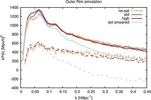
OuterRimN-body simulation power-spectrum monopole (solid lines) and quadrupole (dashed) lines, computed as the mean of 20 realizations. The colours represent different satellite fractions used, no-sat with f = 0 (orange lines), std with f = 0.13 (dark-blue lines), and high with f = 0.22 (red lines), with no smearing. The light blue lines correspond to the smearing case for the fstd satellite fraction. At large scales increasing the satellite fraction increases the amplitude of the monopole, consistent with an enhancement of the linear bias parameter. At small scales, the satellites induce a non-linear damping term consistent with the expected by a intra-halo velocity dispersion. This effect is saturated when the redshift smearing effect is included, making it difficult to distinguish among the cases with different fractions at small scales (not plotted for clarity).
The underlying cosmological model of the or simulations follows a flat ΛCDM with the following parameters, |$\mathbf {\Delta }^{\rm {\small OR}}=\lbrace \Omega _m, \Omega _bh^2,h, \sum m_\nu , \, \sigma _8,n_s\rbrace =\lbrace 0.26479,0.02258,0.71, 0,0.8,0.963\rbrace$|, which is consistent with the WMAP7 cosmology (Komatsu et al. 2011).
Bear in mind that the or-skycuts are derived from a single snapshot at z = 1.433, which does not match the effective redshift5 derived from the DR14Q range (0.8 ≤ z ≤ 2.2). Since here we are interested in using the or just to perform systematic tests on the model, it is not really important that DR14Q and or match perfectly the redshift range. Because of this freedom, we reduce the redshift range of the or-skycut to be 0.8 < z < 2.0, which has an effective redshift of zeff = 1.43, matching the cubic snapshot epoch. With these parameters, the expected value for fσ8 is 0.38216, and the expected values for the αs are 1, as we analyse the or-skycut using the simulated cosmology as fiducial cosmology.
2.3.4 Synthetic observational features
We include the fibre collision and redshift failures in the ez and qpm mocks in order to (i) have a more realistic covariance matrices that match the actual number of observed targets and (ii) quantify the systematic shifts (if any) that the weights described in the Section 2.2.1 produce in the cosmological parameters of interest.
We start by imprinting the same tile distribution of the data in the mocks. In practice, the tile distribution of the data is applied in order to minimize the number of untargeted objects by overlapping the tiles in the densest regions of the survey, which makes the tiling process cluster dependent. We do not follow the same procedure on the mocks, which would require us to run the same algorithm for every mock, producing a different tiling pattern each time. For simplicity, we apply the DR14Q tiling distribution.
We start by assigning each mock particle to a specific plate. In case the mock particle falls in an overlap region, it is randomly assigned to an overlapping plate, but with higher probability of falling to the plates whose centre is closer. The collision pair effect is applied to those particles within 62 arcsec and which both fall into non-overlapping regions (and to those particles that have not been already removed by the close pair selection algorithm). One particle is removed and the other is assigned a +1 wcp weight. The redshift failure effect is applied following the pattern of bottom panels of Fig. 1. We assign the plate coordinates (xfoc, yfoc) to each mock particles and from those a probability of failing (1 − Psuccess). The particles tagged as failure are removed from the catalogue. At the end of these two processes, the remaining particles are assigned a wfoc weight according to the same pattern, as it is done for the DR14Q catalogue.
These two processes do not change the effective number of particles (Neff = ∑iwcpwfoc), although they remove actual particles from the mocks. Since the covariance matrix of the DR14Q sample is dominated by shot noise, by producing the mocks with the same number of particles that the DR14Q catalogue, the covariances derived from the mocks contain the same level of shot noise.
3 METHODOLOGY
3.1 Fiducial cosmology
We analyse all the ez, qpm mocks and data in a flat, ΛCDM cosmological model with |$\mathbf {\Delta }^{\rm fid}=\lbrace \Omega _m, \Omega _bh^2,h, \sum m_\nu , \, \sigma _8,n_s\rbrace =\lbrace 0.31, 0.022, 0.676, 0.06eV, 0.8, 0.97\rbrace$|, which matches the fiducial cosmology used for the BOSS DR12 analysis (Alam et al. 2017) and for the eBOSS DR14Q BAO analysis (Ata et al. 2018). The cosmology of the mocks is similar to the chosen fiducial cosmology and, as a consequence, the expected shift in the dilation scale factors parameter is |$\le {}1\hbox{ per cent}$|.
Table 1 displays the expected values for the dilation scale factors and fσ8 for qpm and ez mocks when analysed under the fiducial cosmology model. Since the ez mocks light-cone is produced using snapshots at different epochs, we display the expected parameters at the different redshift ranges that are later used in the analysis of the data.
Expected values of cosmological parameters for the qpm and ez mocks at different redshift ranges, when analysed using the fiducial cosmology model.
| Type | z-range | zeff | αiso | α∥ | α⊥ | f(z)σ8(z) |
|---|---|---|---|---|---|---|
| ez | 0.8–1.5 | 1.19 | 1.000 72 | 1.001 79 | 1.000 18 | 0.415 82 |
| ez | 1.2–1.8 | 1.50 | 1.001 00 | 1.002 13 | 1.000 43 | 0.380 50 |
| ez | 1.5–2.2 | 1.83 | 1.001 22 | 1.002 37 | 1.000 64 | 0.346 42 |
| ez | 0.8–2.2 | 1.52 | 1.001 01 | 1.002 15 | 1.000 45 | 0.378 36 |
| qpm | 0.8–2.2 | 1.52 | 1.001 08 | 1.001 08 | 1.001 08 | 0.364 32 |
3.2 Power-spectrum estimator
The radial distribution, n(z) of the random catalogue associated with the actual data catalogue, matches the observed NGC and SGC n(z) distributions, plotted in blue and yellow lines in Fig. 2. On the other hand, the n(z) of the random catalogue associated with the quasar mock catalogues matches the smoothed n(z) represented by black dashed lines in Fig. 2. The potential impact on the choice of the degree of smoothing of the n(z) distribution has been previously studied within the BOSS survey (Wang, Guo & Cai 2017 in the context of BAO detection) and within the 2 deg Field Galaxy Redshift Survey (see section 3.1 of Cole et al. 2005b). We have tested the impact of using both set of randoms on the actual DR14Q data catalogue, without observing any significant deviation with respect the typical size of the error-bars. We leave for a future work a more detailed study on the optimal choice of the n(z) of the random catalogue.
In order to measure the power-spectrum multipoles of the quasar distribution, we begin by assigning the objects of the data and random catalogues to a regular Cartesian grid. This approach allows the use of Fourier Transform (FT)-based algorithms. In order to avoid spurious effects of the Cartesian grid, we developed a convenient interpolation scheme to convert particle position in grid overdensity field.
We embed the full survey volume into a cubic box of side Lb = 7200 h−1 Mpc, and subdivide it into |$N_g^3=1024^3$| cubic cells, whose resolution and Nyqvist frequency are 7 h−1 Mpc and kNy = 0.447 h Mpc−1, respectively. We assign the particles to the cubic grid cells using a 5th-order B-spline mass interpolation scheme, where each data/random particle is distributed among 63 surrounding grid cells. Additionally, we interlace two identical grid cells schemes displaced by half of the size of the grid cell; this allow us to reduce the aliasing effect below 0.1 per cent at scales below the Nyqvist frequency (Hockney & Eastwood 1981; Sefusatti et al. 2016).
![Top panel: The DR14 quasar power-spectrum monopole (green), quadrupole (orange), and hexadecapole (purple) in the redshift range 0.8 ≤ z ≤ 2.2, including both NGC and SGC sky patches. The displayed error-bars are the rms of 1000 realizations of the ez mocks. The dashed black lines represent the best-fitting model for the k-range 0.02 ≤ k [h Mpc−1] ≤ 0.30. The bottom sub-panel shows the differences between the model and data, divided by the diagonal errors, using the same colour scheme. The 2σ and 3σ confidence levels are marked with dashed and dotted black lines, respectively. Bottom panel: Monopole and quadrupole measurement of the data for the different redshift estimates described in Section 2.1.1: zfid in black symbols, $z_{\rm Mg\, {{\small II}}}$ in red symbols, and zPCA in blue symbols. The bottom sub-panels display the difference with respect to the fiducial redshift estimate relative to the statistical errors for the monopole and quadrupole. For clarity, we do not display the results for the hexadecapole, where the degree of agreement is similar to the other two multipoles.](https://oup.silverchair-cdn.com/oup/backfile/Content_public/Journal/mnras/477/2/10.1093_mnras_sty453/2/m_sty453fig5.jpeg?Expires=1716429279&Signature=qHRZkgEA~GCxV1NBUrgtVeWqW-DwNFZeU6HogplQLSIEBnfNDNSXHjH59-MMi7DMycPlewzHLzEFMhXx-9MMEqph06NxCMq4jCFIWtT6DELTzdojtoGr-oS5uPOgs94Sx3DQlkRn5y3G34N7SGBOCYCaVwvi2rhjE6ZgEON-v6s5~G350qgKU~GIVEjGM9JnIJZB0pIo8bfkJ6GZVz1FmDhpRL1udP3bCnjJREB5VKR-aOM8Gn2oRxvby3NIwUcb2tv4LLItzajwSIQkJTuqVYf2M-XLIE6zD4w1ux35W-AGOqt9Y8u7x75vdWcOa3J2xeMc8wgS7Y3Irge0YvKmjQ__&Key-Pair-Id=APKAIE5G5CRDK6RD3PGA)
Top panel: The DR14 quasar power-spectrum monopole (green), quadrupole (orange), and hexadecapole (purple) in the redshift range 0.8 ≤ z ≤ 2.2, including both NGC and SGC sky patches. The displayed error-bars are the rms of 1000 realizations of the ez mocks. The dashed black lines represent the best-fitting model for the k-range 0.02 ≤ k [h Mpc−1] ≤ 0.30. The bottom sub-panel shows the differences between the model and data, divided by the diagonal errors, using the same colour scheme. The 2σ and 3σ confidence levels are marked with dashed and dotted black lines, respectively. Bottom panel: Monopole and quadrupole measurement of the data for the different redshift estimates described in Section 2.1.1: zfid in black symbols, |$z_{\rm Mg\, {{\small II}}}$| in red symbols, and zPCA in blue symbols. The bottom sub-panels display the difference with respect to the fiducial redshift estimate relative to the statistical errors for the monopole and quadrupole. For clarity, we do not display the results for the hexadecapole, where the degree of agreement is similar to the other two multipoles.
3.3 Modelling
The theoretical model used in this paper to describe the power-spectrum multipoles is identical to the one used in previous analyses of the BOSS survey for the redshift range 0.15 < z < 0.70 (Gil-Marín et al. 2015; Gil-Marín et al. 2016), so we briefly present the model without details to avoid repetition. We refer the reader to the references of this section for a further description.
3.3.1 Bias model
We assume the Eulerian non-linear bias model presented by McDonald & Roy (2009). The model has four bias parameters: the linear bias b1, the non-linear bias b2, and two non-local bias parameters, |$b_{s^2}$| and b3nl. As in previous works, we assume b1 and b2 to be free parameters of the model. The remaining two non-local bias parameters can be constrained by assuming that the bias model is local in Lagrangian space, which sets |$b_{s^2}$| and b3nl as a function of b1: |$b_{s^2}=-4/7\,(b_1-1)$| (Baldauf et al. 2012) and b3nl = 32/315 (b1 − 1) (Saito et al. 2014).
3.3.2 Redshift space distortions
We model the redshift space distortions in the power-spectrum multipoles following the approach presented by Taruya, Nishimichi & Saito (2010) (TNS model). We assume that there is no velocity bias between the galaxy field and the underlying dark matter field, at least on the scale of interest for this paper. The TNS model provides a prescription for the redshift space power spectrum in terms of the real space quantities: the matter–matter, velocity–velocity, and the cross-matter–velocity non-linear power spectra. These non-linear quantities are computed using the resumed perturbation theory at two-loop order as described in Gil-Marín et al. (2012). All these non-linear power-spectrum quantities are fuelled with the linear matter power spectrum computed using camb (Lewis, Challinor & Lasenby 2000). The power-spectrum multipoles encode the coherent velocity field through the redshift space displacement and the logarithmic growth of structure parameter, |$f\equiv \frac{\text{d}\log D(z)}{\text{d}\log a(z)}$|. The effect of this parameter is to increase the clustering along the LOS with respect to the transverse direction, boosting the amplitude of the isotropic power spectrum and generating an anisotropic component.
3.3.3 The Alcock–Paczynski effect
The dilation scale factors α∥ and α⊥ describe how the true frequencies k΄ have been distorted into the observed ones k, (|$k_\parallel =\alpha _\parallel k^{\prime }_\parallel$| and |$k_\perp =\alpha _\perp k^{\prime }_\perp$|), by the effect of assuming an incorrect cosmological model.
Table 2 displays the fiducial values for DA, H, and DV for the different cosmologies used in this paper at their effective redshifts.
Values of the BAO isotropic distance, DV, the angular diameter distance DA, the Hubble parameter H and the sound horizon at drag redshift, rs(zd) for the fiducial, ez- and qpm-mock true cosmology at their effective redshifts, zeff = 1.52 for fiducial and ez mocks, and zeff = 1.51 for qpm mocks. Units of DV, DA, and rs are in Mpc, whereas H is in km s−1 Mpc−1.
| DV(zeff) | H(zeff) | DA(zeff) | rs | |
|---|---|---|---|---|
| Fiducial | 3871.0 | 160.70 | 1794.7 | 147.78 |
| qpm mocks | 3858.5 | 159.85 | 1794.4 | 147.62 |
| ez mocks | 3871.8 | 160.48 | 1794.1 | 147.66 |
| DV(zeff) | H(zeff) | DA(zeff) | rs | |
|---|---|---|---|---|
| Fiducial | 3871.0 | 160.70 | 1794.7 | 147.78 |
| qpm mocks | 3858.5 | 159.85 | 1794.4 | 147.62 |
| ez mocks | 3871.8 | 160.48 | 1794.1 | 147.66 |
3.3.4 Survey geometry
The last step to be included in the model is the effect of the window function produced by the non-uniform distribution of quasars, both angularly and radially. We account this effect by following the procedure described by Wilson et al. (2017). In practise, the window has two main effects: (i) to reduce the observed power at large scales, being more severe as one increases the value of the ℓ-multipole and (ii) to increase the covariance among adjacent k-modes, specially at large scales. We follow the same formalism used by Beutler et al. (2017), which is fully described in Appendix B.
3.3.5 Free parameters of the model
In addition to the free parameters of the model described above, we also marginalize over the amplitude of the linear power spectrum through the amplitude of the dark matter fluctuations filtered with a top-hat filter of 8 Mpc, σ8(z). This parameter is highly degenerate with other parameters such as the bias parameters and the logarithmic growth of structure. Thus, we set σ8 to the fiducial value of our cosmology in the non-linear terms of the model, and constrain the combination of σ8 times the bias parameters or the logarithmic growth of structure from the large-scale modes.
To summarize, the full power-spectrum model described in the sections above has seven free parameters: two bias parameters, b1σ8 and b2σ8; two nuisance parameters, Anoise and σP; and three cosmological parameters, fσ8, α∥, and α⊥. For those cases where ε is set to 0, α⊥ = α∥ ≡ αiso, and the number of free parameters is reduced by one.
3.4 Parameter estimation
The covariance matrix is computed using a large number of mock quasar samples described in Section 2.3. For our fiducial results, we use the 1000 realizations of the ez mocks, unless otherwise noted. Due to the finite number of mock realizations when estimating the covariance, we expect a noise term to be present that requires a correction to the final χ2 values. We apply the corrections described in Hartlap, Simon & Schneider (2007). Such corrections represent a |${\sim }15\hbox{ per cent}$| factor in the χ2 values; we use 1000 mock realizations to estimate the full covariance of 84 k-bins, including monopole quadrupole and hexadecapole. We do not apply any extra corrections, such the ones described in Percival et al. (2014), which have a minor contribution to the final errors.
Using a simplex minimization algorithm (Nelder & Mead 1965; Press et al. 2002), we explore the surface of the likelihood function to find the best-fitting value for each of the p-parameters and its 1σ marginalized error. We ensure that the minima found are global and not local by running the algorithm multiple times with different starting points and different variation ranges.
As mentioned above, the value of σ8 is set constant to its fiducial value in the non-linear terms of the model, so the parameter fσ8 is effectively fitted. We have checked that due to the high degree of degeneracy between f and σ8, the impact of following this procedure does not change our results for physical values of σ8.
In order to compute the full likelihood surface of a set of parameters, we also run Markov chains (mcmc chains). We use a simple Metropolis–Hasting algorithm with a proposal covariance and ensure its convergence performing the Gelman–Rubin convergence test, R − 1 < 10−3, on each parameter. We apply the flat priors listed in Table 3 otherwise stated.
Flat priors ranges on the parameters of the model. The priors on α∥ and α⊥ are modified when the three redshift bins are analysed as described in Table 10. Since σ8 is fixed to its fiducial value during the fit (see the text), the priors are effectively applied to the parameters f, b1, and b2. In order to obtain the priors on fσ8, b1σ8, and b2σ8, the priors need to be re-scaled by the fiducial value of σ8, 0.397.
| Parameter | Flat prior range |
|---|---|
| αiso | [0, 2] |
| α∥ | [0, 2] |
| α⊥ | [0, 2] |
| f | [0, 5] |
| b1 | [0, 5] |
| b2 | [ − 10, 10] |
| σP | [0, 30] |
| 10−3Anoise | [ − 1, 1] |
| Parameter | Flat prior range |
|---|---|
| αiso | [0, 2] |
| α∥ | [0, 2] |
| α⊥ | [0, 2] |
| f | [0, 5] |
| b1 | [0, 5] |
| b2 | [ − 10, 10] |
| σP | [0, 30] |
| 10−3Anoise | [ − 1, 1] |
4 MEASUREMENTS
In this section, we present the measurement of the power-spectrum multipoles of the DR14 quasar sample, as well as the performance of the model and the mocks. We start by discussing the measurements in the whole redshift bin, 0.8 ≤ z ≤ 2.2; and we later divide the full redshift range into three overlapping redshift bins: lowz, 0.8 ≤ z ≤ 1.5; midz, 1.2 ≤ z ≤ 1.8; highz, 1.5 ≤ z ≤ 2.2. Following the second approach, we are in principle sensitive to redshift-evolution quantities, such as b1(z)σ8(z) and f(z)σ8(z). In Section 7, we will explore how the two different approaches, the single and multiple redshift bins, performed when constraining cosmological parameters.
4.1 Single redshift bin
The top panel of Fig. 5 displays the DR14Q measured power-spectrum monopole (green circles), quadrupole (orange squares), and hexadecapole (purple triangles) in the redshift range of 0.8 ≤ z ≤ 2.2. The error-bars correspond to the diagonal elements of the covariance matrix estimated from the rms of the 1000 realizations of the ez mocks. The black dashed lines represent the best-fitting theoretical model. Although the power spectrum has been measured in the range 0 < k [h Mpc−1] < 0.40, only those k-bins in the range 0.02 < k [h Mpc−1] < 0.30 have been used to fit the theoretical model; therefore, the black dashed lines only cover this specific range. The lower sub-panels display the difference between the measured power spectrum and the best-fitting theoretical model divided by the 1σ error. The associated χ2 with this fit is 84.0/(84 − 7). The contribution from the monopole-only data points is |$\chi ^2_{P^{(0)}}=20.1/(28-7)$|, from the quadrupole |$\chi ^2_{P^{(2)}}=30.2/(28-6)$|, and from the hexadecapole |$\chi ^2_{P^{(4)}}=34.6/(28-4)$|.8 Ignoring the covariance between the multipoles would reduce the χ2 by just 0.9, suggesting that the three power-spectrum multipoles are barely correlated (see Fig. D1 in Appendix D for a further description of the correlation among k-bins).
The bottom panel of Fig. 5 displays the impact of changing the redshift estimate of the DR14Q sample from its fiducial methodology, zfid to the one based on the maximum of the Mg ii line, |$z_{\rm Mg\, {\small II}}$| (red symbols) and to the one based on the PCA decomposition technique that also uses the position of the Mg ii line, zPCA (blue symbols). The three redshift estimates display a consistent behaviour for both the monopole and quadrupole, not revealing any specific systematic trend, and the differences on specific k-modes are always below 2σ. We must bear in mind that these measurements must be correlated up to some extent, and therefore we cannot quantify in terms of χ2 the agreement among them, nor their correlation, as we lack different redshift estimates for the mocks. Producing mocks that capture such behaviour would require a simulation of realistic quasar spectra at a given redshift for each particle in the mocks, which is beyond the scope of this paper. For simplicity, we do not show the hexadecapole measurements, as the degree of agreement is similar to the one found in the monopole and quadrupole. In Section 6, we will present the cosmological derived parameters based on these three redshift estimates.
The top panel of Fig. 6 shows the power-spectrum monopole and quadrupole measured on the NGC and SGC separately. Since the two samples are well disconnected they can be considered fully independent. The different colours and symbols distinguish between the NGC and SGC region and the power-spectrum multipole, as indicated. The best-fitting theoretical model is indicated by a solid black line for NGC, and a dashed black line for SGC. The middle and lower sub-panels display the difference between the model and the data divided by the corresponding 1σ error. For clarity, we do not induce the results on the hexadecapole.
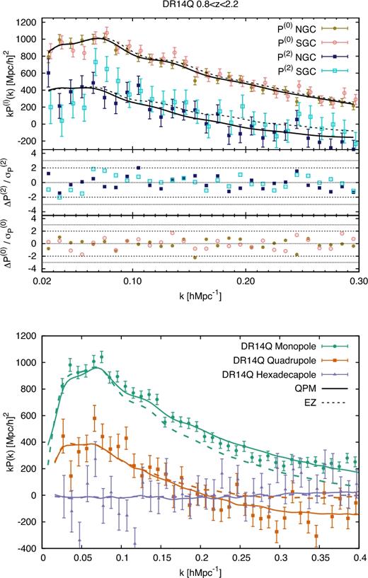
Top panel: DR14 quasar sample measurement for the power-spectrum monopole (circle symbols) and quadrupole (square symbols), for the NGC region (filled symbols) and SGC region (empty symbols) using the full redshift range, 0.8 ≤ z ≤ 2.2. The solid and dashed lines indicate the best-fitting model for the NGC and SGC, respectively. The error-bars display the rms from the ez mocks. The middle and bottom sub-panels display the difference between the model and the measurement divided by the errors, for the quadrupole and monopole, respectively. The horizontal dashed and dotted lines represent the 2 and 3σ confidence levels. Bottom panel: The measured DR14Q data power-spectrum monopole, quadrupole, and hexadecapole are shown for the NGC+SGC region in green, orange, and purple, respectively. The solid and dotted curves are the measured multipoles from the mean of the qpm (400 realizations) and ez mocks (1000 realizations), respectively, using the same colour notation. Since the error-bar for the mean of the mocks is small, it is not plotted. At large scales, both mocks and data show a good agreement, but at small scales, both qpm and ez mocks fail to accurately reproduce the data. However, this behaviour can be partially fixed in the monopole by modifying the shot noise value of the mocks, as it demonstrated in fig. 6 of Ata et al. (2018).
We observe that the data from the SGC presents a slightly higher amplitude than in the NGC, especially for k ≳ 0.15 h Mpc−1 and in the quadrupole. This effect translates into a best-fitting theoretical model with higher bias in the SGC quadrupole. In Section 6, we will quantify this discrepancy and conclude that these differences are not statistically significant. As for the combined NGC+SGC sample, there is no k-bin that deviates more than 3σ with respect to the prediction of the model, and just three points at more than 2σ. The χ2 values for NGC and SGC are 64.5/(84 − 7) and 76.6/(84 − 7), respectively. For the NGC, the separate contribution for the monopole, quadrupole, and hexadecapole are |$\chi ^2_{P^{(0)}}=19.8/(28-7)$|, |$\chi ^2_{P^{(2)}}=22.0/(28-6),$| and |$\chi ^2_{P^{(4)}}=25.0/(28-4)$|; and for the SGC |$\chi ^2_{P^{(0)}}=25.6/(28-7)$|, |$\chi ^2_{P^{(2)}}=24.0/(28-6),$| and |$\chi ^2_{P^{(4)}}=27.6/(28-6)$|.
The bottom panel of Fig. 6 displays the performance of the mean of the 1000 realizations of the ez mocks (dashed lines) and the mean of the 400 realizations of the qpm mocks (solid lines) along with the DR14Q measurements. For the monopole, the ez and qpm underestimate and overestimate, respectively, the measurement from the data. This behaviour was also reported the fig. 6 of Ata et al. (2018).9 When a constant value is added to the mocks, the agreement improves significantly. We also observe differences in the behaviour of the quadrupole at small scales, k > 0.20 h Mpc−1, where the ez mocks tend to overestimate the DR14Q measurements. The hexadecapole measurements are similar for both ez and qpm mocks, and consistent along with the data. In Section 5.3, we quantify the impact of these two covariance matrices in the cosmological parameters of interest.
4.2 Multiple redshift bins
In the previous section, we have presented the measured power-spectrum multipoles for the entire redshift bin, 0.8 ≤ z ≤ 2.2, with an effective redshift of zeff = 1.52. However, the size of this redshift bin is large, which covers a wide range of epochs. During these epochs, we expect that the cosmological parameters, such as fσ8 and b1σ8, will significantly evolve with redshift. Constraining the evolution of these parameters with redshift will better constrain potential departures from the standard cosmological model than just the average measurements of the whole redshift bin.
Following this approach, we divide the DR14Q NGC+SGC sample in three overlapping redshift bins with similar effective volumes: lowz, which covers 0.8 ≤ z ≤ 1.5 and whose effective volume is |$V_{\rm eff}^{lowz}=0.126\,{\rm Gpc}^3$|; midz, which covers 1.2 ≤ z ≤ 1.8 and whose effective volume is |$V_{\rm eff}^{midz}=0.131\,{\rm Gpc}^3$|; and highz, which covers 1.5 ≤ z ≤ 2.2 and whose effective volume is |$V_{\rm eff}^{highz}=0.119\,{\rm Gpc}^3$|. Since the midz range overlaps with both lowz and highz, we expect a significant correlation among these measurements, and their derived cosmological parameters. Using the ez mocks, which contain an intrinsic evolution of the bias and cosmological parameters with redshift, we can compute the cross-correlation coefficients among the parameters of the different redshift bins.
The three panels of Fig. 7 display the power-spectrum monopole (left-hand panel), quadrupole (middle panel), and hexadecapole (right-hand panel) for the DR14Q, for the different redshift bins, as indicated, in the coloured symbols. The coloured dashed lines indicate the best-fitting model, with the same colour notation.
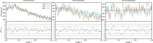
Power-spectrum monopole (left-hand panel), quadrupole (middle panel), and hexadecapole (right-hand panel), for different z-bins: lowz 0.8 ≤ z ≤ 1.5 (green), midz 1.2 ≤ z ≤ 1.8 (purple), highz 1.5 ≤ z ≤ 2.2 (orange). The coloured symbols display the measurements from the NGC+SGC DR14Q sample, whereas the dashed lines indicate the best-fitting model. The lower sub-panels show the differences between the model and the data in terms of 1σ confidence levels.
For the power-spectrum monopole, at large scales the amplitude of the power spectrum increases with redshift. The Kaiser boost factor for the monopole is ([b1σ8]2 + 2/3[fσ8][b1σ8] + 1/5[fσ8]2). The quantity b1σ8(z) is a slightly increasing function with redshift in 0.8 ≤ z ≤ 2.2 (b1 increases with z and σ8 decreases), whereas fσ8(z) is a decreasing function with redshift. However, the bias has a dominant effect over the logarithmic growth factor, and the overall effect is an increase of the amplitude, as observed on the data. At small scales, we observe the opposite effect: the highz redshift bin presents a more important damping factor than the lowz bin. This behaviour is also expected, as the parameter σP in our model accounts not only for the damping caused by the intra-halo velocity dispersion of the satellite quasars but also for the effect of spectroscopic redshift errors. It is expected that these errors will increase with redshift, as the more distant objects tend to have lower signal-to-noise ratio spectra, which can lead to significant errors in the measurement of their radial distance (see the Gaussian smearing redshift error model at the end of Section 2.3.1).
For the power-spectrum quadrupole, we observe the opposite behaviour at large scales. In this case, the Kaiser boost factor becomes, (4/3[b1σ8][fσ8] + 4/7[fσ8]2), where the dominant component is fσ8(z), which drives the whole factor to decrease with redshift, as seen in the data and best-fitting model. Indeed, the importance of the bias parameters decreases for high-order multipoles, which causes the Kaiser boost factor to be dominated by the z-evolution of the fσ8(z) parameter. At small scales, we observe the same behaviour in the monopole. The redshift failure effects that produce that the damping factor strongly increase with redshift.
Finally, in the hexadecapole the Kaiser boost factor is ∝ [fσ8]2, with no bias contribution at large scales. Because of the large statistical errors, we do not observe any particular trend of the hexadecapole as a function of the redshift bin. In addition, in the midz redshift bin, the hexadecapole at k ∼ 0.11 h Mpc−1 is a 4σ outlier with respect to the expected model. This tension is reduced to the 3σ discrepancy when the full redshift range is considered, as shown in the top panel of Fig. 5. In Section 6.3, we will discuss the impact of this frequency in the total χ2 and in the cosmological parameters.
5 SYSTEMATIC TESTS
We aim to identify potential systematic errors of our model, as well as potential systematics on the data, and quantify their effect on the measurements of cosmological interest. We start by using the ez and qpm mocks to recover the expected cosmological parameters. Although these mocks are not a proper N-body simulation, they can provide a first approximation on the performance of how the model works at these redshifts, and, more importantly, can test the effect of the potential systematics introduced by the spectroscopic weights. We will later use the OuterRimN-body simulations to test the performance of the model using different prescriptions for the fraction of satellite quasars.
5.1 Isotropic fits on mocks
Table 4 displays the shifts between the measured αiso and fσ8 parameters, and the expected value from the known cosmology of the mocks and or-skycut, when ε is fixed to 0. The expected values for both qpm and ez mocks can be found in Table 1. For or, the expected αiso is 1 as explained in Section 2.3.3. The 〈x〉i rows contain those quantities obtained by fitting the mean of all available realizations. In this case, the errors represent the errors of the mean, where all the elements of the covariance matrix have been re-scaled by the inverse of the total number of realizations 1000, 400, and 20 for the ez, qpm, and or-skycut mocks, respectively. The 〈xi〉 rows are the average of the best-fitting parameters individually on each realization. In this case, the errors represent the average of the errors of each individual fit. Additionally, the S columns display the rms among best-fitting values of αiso and fσ8 of each realization. The Ndet column is the number of mocks whose best-fitting values for αiso lie between 0.8 and 1.2. We consider those realizations as mocks with detection of αiso (this is the same definition in table 4 of Ata et al. 2018). The average quantities 〈fσ8i〉 and 〈αisoi〉 (as well as the respective Si) are computed only using these ‘detection’ realizations, and discarding the rest. The Δαiso, Δfσ8, and S values are expressed in terms of 10−2 units. Thus, Δx = 1 corresponds, for instance, to a shift of 0.01 with respect to the true expected value.
Shifts on the cosmological parameters, x, with respect to their expected value, xexp, Δx ≡ x − xexp; for x = αiso and x = fσ8 on ez and qpm mocks in the redshift range 0.8 ≤ z ≤ 2.2 and on the or-skycut mock in 0.8 ≤ z ≤ 2.0. 〈xi〉 quantities are the average of the best-fitting values measured in individual realizations, whereas 〈x〉i are the quantities obtained by fitting the average of all the realizations. The errors correspond to the average value of the errors of individual fits and the error of the mean, in each case. For the 〈xi〉 rows, the average is only performed among those realizations whose best-fitting value for αiso are between 0.8 and 1.2, for the αiso and fσ8 columns. We call such fits a detection. The number of detection realizations is presented by the column Ndet. The Sx columns display the rms of αiso and fσ8, as indicated by the sub-index i. The units of Δx and Sx are 10−2, such that Δx = 1 corresponds to a shift of 0.01. All results use the 0.02 ≤ k [h Mpc−1] ≤ 0.30 range for the fits. For both qpm and ez mocks, the covariance elements have been computed using their own covariance, unless the contrary is explicitly stated. For the or-skycut mocks, the NGC ez covariance is used and is re-scaled to match the rms of the diagonal elements of the 20 or-skycut mock realizations. Additionally, we also present the effect of correcting the spectroscopic effects of fibre collision and redshift failures on the ez and qpm mocks (see the text for full description and notation), where the rows labelled ‘raw’ are those corresponding to the mocks with no observational effects applied. For the or-skycut mocks, no observational effects, other than a selection function, is applied.
| Δαiso | Sα | Δfσ8 | |$S_{f\sigma _8}$| | Ndet | |
|---|---|---|---|---|---|
| ez mocks | |||||
| 〈x〉i raw | −1.64 ± 0.13 | − | −1.14 ± 0.16 | − | − |
| 〈x〉iwnozwcp | −1.90 ± 0.13 | − | 2.53 ± 0.17 | − | − |
| 〈x〉izf | −1.73 ± 0.13 | − | −1.30 ± 0.16 | − | − |
| 〈x〉iwfocwcp | −1.80 ± 0.13 | − | −0.19 ± 0.16 | − | − |
| 〈x〉iwfocwcpqpm-Cov | −1.90 ± 0.12 | − | −0.06 ± 0.16 | − | − |
| 〈x〉iwfocwcp + P(4) | −1.64 ± 0.13 | − | −0.10 ± 0.17 | − | − |
| 〈xi〉 raw | −1.65 ± 3.91 | 4.41 | −1.09 ± 4.89 | 4.91 | 979 |
| 〈xi〉 wfocwcp | −1.63 ± 4.16 | 4.47 | −0.03 ± 5.24 | 5.12 | 973 |
| 〈xi〉 wfocwcpqpm-Cov | −1.69 ± 3.94 | 4.83 | +0.12 ± 5.12 | 5.69 | 945 |
| 〈xi〉 wfocwcp + P(4) | −1.49 ± 4.16 | 4.43 | −0.03 ± 5.30 | 5.10 | 970 |
| qpm mocks | |||||
| 〈x〉i raw | 0.28 ± 0.22 | − | 0.51 ± 0.21 | − | − |
| 〈x〉iwfocwcp | 0.15 ± 0.21 | − | 1.05 ± 0.24 | − | − |
| 〈xi〉 raw | 0.37 ± 4.1 | 4.48 | 0.84 ± 4.4 | 4.21 | 397 |
| 〈xi〉 wfocwcp | −0.28 ± 4.4 | 4.84 | 1.57 ± 5.0 | 4.80 | 396 |
| or-skycut mock w/o smearing | |||||
| no-sat 〈x〉i | 0.46 ± 0.79 | − | −1.25 ± 0.95 | − | − |
| std 〈x〉i | −1.80 ± 0.75 | − | −1.77 ± 0.86 | − | − |
| high 〈x〉i | −2.33 ± 0.64 | − | −1.02 ± 0.80 | − | − |
| or-skycut mock w/ smearing | |||||
| no-sat 〈x〉i | 0.82 ± 0.84 | − | −0.63 ± 1.02 | − | − |
| std 〈x〉i | −0.86 ± 0.75 | − | −0.60 ± 0.94 | − | − |
| high 〈x〉i | −2.05 ± 0.66 | − | 0.37 ± 0.88 | − | − |
For the ez and qpm mock cases, the rows labelled with ‘raw’ correspond to those results obtained when no spectroscopic effects, such redshift failures and fibre collision, are added (and therefore there is no need for these corrections). The rows labelled with zf correspond to those mocks with the redshift failure effect applied and corrected using the wfoc weight (according to equation 2). Those rows labelled as wfocwcp refer to mocks where both fibre collisions and redshift failures are applied and corrected following the prescription described in Section 2.2.1. The rows labelled as wnozwcp also contain both fibre collisions and redshift failures, but in this case, the redshift failures have been corrected using the near-neighbour technique. Those rows noted as +P(4) represent the analysis including the hexadecapole signal. The ez and qpm mocks are analysed using their own covariance. However, the ez mocks also include the case where the qpm-derived covariance is used in order to test its impact.
In general, there is a concordance between the shifts observed for the 〈xi〉 and 〈x〉i variables. The αiso variable is robust under the different analysis methods, and we observe a consistent |$1\text{--}2\hbox{ per cent}$| shift for the ez mocks to systematically lower values than expected, and |$<{}1\hbox{ per cent}$| shift for the qpm mocks. The systematic |$1\text{--}2\hbox{ per cent}$| shift observed on the ez mocks (and not observed in the qpm) may be due to either some systematic of the model or an intrinsic systematic of the mocks.
The fσ8 variable is more sensitive to the spectroscopic weights, in particular, to the redshift failures when they are corrected through the wnoz prescription. In this case, the systematic shifts on fσ8 can reach |${\sim }6\hbox{ per cent}$|, whereas the correction through wfoc does not produce any measurable systematic shift. Moreover, the impact of fibre collisions through the wcp weight correction is |$<{}2\hbox{ per cent}$|. Adding the hexadecapole does not produce any significant change on the fits. This is because we are performing fits with ε set to 0, whereas the main extra information of the hexadecapole comes for breaking the degeneracy among α∥ and α⊥. By adding the spectroscopic weights, the errors and the rms values increase because of the increase of the shot noise component in the covariance matrix, which is the dominant term. Finally, the fits on the ez mocks with either the ez-derived covariance matrix or the qpm-derived covariance matrix do not produce any significant shift.
The or-skycut mock results are also displayed in the lower columns of Table 4 for three different satellite fraction, fno-sat = 0, fstd = 0.13 and fhigh = 0.22, and with and without a redshift smearing effect, which would mimic the expected uncertainty in the model determination. The qpm mocks, which are also based on a HOD technique, have a satellite fraction similar to fstd. For the or-skycut mock analyses, no fibre collision or redshift failure effect has been included. The or-skycut mock results show that neither the satellite fraction nor the redshift error smearing has an important impact on fσ8; the systematic shifts are below |${\sim } 4\hbox{ per cent}$| (shift of ≤0.02). Similarly, the value of the αiso parameter does not produce shifts higher than |$2\hbox{ per cent}$|, although the systematic shift increases as the satellite fraction increases.
The upper panel of Fig. 8 displays the distribution of the best-fitting solution corresponding to the 1000 realizations of the ez mocks with the wfocwcp weights applied (blue circles) and DR14Q data (for the same weighting scheme) for the different redshift estimates: zfid (orange cross), |$z_{\rm Mg \,{{\small II}}}$| (red cross), and zPCA (black cross) for the parameters αiso, fσ8, and b1σ8; as well as the corresponding histograms including the χ2 distribution. The figure shows the degeneracies among parameters, in particular the strong correlation between αiso and b1σ8, as both parameters are sensitive to the amplitude of the power spectrum at all scales. Given these results, the data accordingly fit into a typical realization of the mocks, and all the redshift estimates provide similar results on the studied parameters. The bottom panel of Fig. 8 displays the distribution of the 1σ error for αiso in the x-axis and fσ8 in the y-axis. The mocks show a positive correlation between the error of fσ8 and αiso, as expected, since αiso and fσ8 are correlated as well, i.e. αiso is well determined in a particular realization, the probability that fσ8 is well determined in that particular realization is high. The errors measured from the data when zfid and zPCA are used are consistent with the mocks. The measured errors on the data with redshift estimate |$z_{\rm Mg\, {\small II}}$| are ∼2σ larger than the distribution of the mocks. This behaviour may be caused by the broadening on spectroscopic redshift errors when estimating the redshifts using the Mg ii line with respect to the other two methodologies.
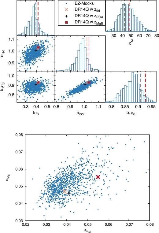
Top panel: Best-fitting solution for the 1000 realizations of the ez mocks (in blue circles) and DR14Q data set: orange cross for zfid, red for |$z_{\rm Mg\, {\small II}}$|, and black for zPCA, under the constraint ε = 0 for the parameters b1σ8, fσ8, αiso when the power-spectrum monopole and quadrupole are used. The histograms show the distribution of parameters, as well as the χ2 values. The panels display the correlation among parameters. Bottom panel: Distribution of the 1σ errors of the fσ8 and αiso parameters, for the ez mocks in blue circles, and DR14Q data using the same colour notation. The uncertainty of fσ8 and αiso parameters have a positive correlation. In both panels, the results from the DR14Q data, when the zfid and zPCA estimates are used, are a typical individual case of the mocks. The errors obtained from the |$z_{\rm Mg\, {\small II}}$| redshift estimates are ∼2σ larger than those expected from the mocks.
5.2 Anisotropic fits on mocks
In this section, we extend the above tests by relaxing the ε = 0 prior. We refer to the fit under these conditions as ‘full-AP’ fit. The results are shown in Table 5 for the ez, qpm, and or-skycut mocks, similarly as it was presented in the previous section.
Shifts of α∥, α⊥, and fσ8 with respect to the fiducial values when the full-AP test is performed. The notation is the same that the one used in Table 4, with the difference that the definition of detection has been relaxed to be 0.7 < α < 1.3. Fig. 10 summarizes the systematics shifts observed in this table.
| Δα∥ | Sα | Δα⊥ | Sα | Δfσ8 | |$S_{f\sigma _8}$| | Ndet | |
|---|---|---|---|---|---|---|---|
| ez mocks | |||||||
| 〈x〉i raw | −1.58 ± 0.30 | − | −1.71 ± 0.20 | − | −1.29 ± 0.25 | − | − |
| 〈x〉izf | −1.67 ± 0.31 | − | −1.75 ± 0.21 | − | −1.40 ± 0.26 | − | − |
| 〈x〉iwfocwcp | −2.02 ± 0.31 | − | −1.69 ± 0.22 | − | −0.13 ± 0.27 | − | − |
| 〈x〉i raw + P(4) | −2.24 ± 0.23 | − | −1.33 ± 0.17 | − | −0.82 ± 0.21 | − | − |
| 〈x〉iwfocwcp + P(4) | −4.36 ± 0.24 | − | 0.03 ± 0.19 | − | 1.92 ± 0.23 | − | − |
| 〈x〉izf +P(4) | −2.28 ± 0.24 | − | −1.38 ± 0.18 | − | −0.94 ± 0.22 | − | − |
| 〈xi〉 raw | −1.61 ± 9.64 | 8.11 | −1.69 ± 6.13 | 6.80 | −1.18 ± 8.06 | 8.20 | 809 |
| 〈xi〉 raw + P(4) | −2.50 ± 7.72 | 7.53 | −1.44 ± 5.38 | 6.34 | −0.56 ± 6.76 | 7.18 | 951 |
| 〈xi〉 wfocwcp + P(4) | −4.36 ± 8.32 | 7.70 | 0.10 ± 5.85 | 6.26 | 2.31 ± 7.44 | 7.39 | 902 |
| qpm mocks | |||||||
| 〈x〉i raw | 1.12 ± 0.47 | − | 0.25 ± 0.35 | − | 0.19 ± 0.41 | − | − |
| 〈x〉iwfocwcp | 0.22 ± 0.53 | − | 0.13 ± 0.36 | − | 0.87 ± 0.43 | − | − |
| 〈x〉i raw + P(4) | 1.18 ± 0.39 | − | 0.39 ± 0.30 | − | −0.14 ± 0.33 | − | − |
| 〈x〉iwfocwcp + P(4) | −1.34 ± 0.44 | − | 1.61 ± 0.33 | − | 1.88 ± 0.37 | − | − |
| 〈xi〉 raw | 0.94 ± 11.03 | 8.03 | 0.70 ± 6.27 | 7.24 | 1.26 ± 8.03 | 7.64 | 307 |
| 〈xi〉 raw + P(4) | 0.63 ± 8.87 | 8.09 | 0.27 ± 4.92 | 7.37 | 0.93 ± 6.48 | 7.57 | 345 |
| 〈xi〉 wfocwcp + P(4) | −2.43 ± 8.15 | 8.77 | 0.63 ± 4.89 | 8.43 | 2.61 ± 6.53 | 9.46 | 326 |
| or-skycut w/o smearing | |||||||
| 〈x〉i no-sat +P(4) | −0.07 ± 1.28 | − | 0.83 ± 1.04 | − | −0.89 ± 1.38 | − | − |
| 〈x〉i std +P(4) | −1.12 ± 1.27 | − | −2.23 ± 0.94 | − | −2.69 ± 1.30 | − | − |
| 〈x〉i high +P(4) | −3.09 ± 1.08 | − | −2.11 ± 0.84 | − | −0.39 ± 1.20 | − | − |
| or-skycut w/ smearing | |||||||
| 〈x〉i no-sat +P(4) | 0.28 ± 1.56 | − | 1.03 ± 1.13 | − | −0.45 ± 1.48 | − | − |
| 〈x〉i std +P(4) | 1.50 ± 1.63 | − | −1.82 ± 0.99 | − | −2.91 ± 1.41 | − | − |
| 〈x〉i high +P(4) | −2.13 ± 1.28 | − | −2.35 ± 0.86 | − | 0.09 ± 1.24 | − | − |
We start by describing the results on the ez and qpm mocks. When the power-spectrum monopole and quadrupole are used, the results on the ‘raw’ mocks present less than |$2\text{--}3\hbox{ per cent}$| systematic shifts, similar to what was observed in the isotropic case. By including the hexadecapole on the ez mocks, there is a slight increase on the systematics of the α∥ parameter, which reaches a |$2.5\hbox{ per cent}$| shift, but it does not have any effect on the rest of parameters or on the qpm mocks, other than reducing the statistical uncertainty by |${\sim }20\hbox{ per cent}$|.
We compare the observed shifts on the ‘raw’ mocks with the rest of the mocks using different weigh-based prescriptions. In the zf case, the wfoc weight perfectly accounts for the redshift failure effects (see also in Appendix C the effect on the signal from the power-spectrum multipoles), even when the hexadecapole signal is considered. For the wfocwcp case, when only the power-spectrum monopole and quadrupole are considered the inferred cosmological parameters shift slightly more than |$1\hbox{ per cent}$| both for ez and qpm mocks. When the hexadecapole is added, we observe a systematic |$2\hbox{ per cent}$| for both ez and qpm mocks towards lower values of α∥; |${\lesssim }1\hbox{ per cent}$| shift on α⊥ towards higher values; and ∼0.02 shift towards higher values of fσ8, which represent a |${\sim }5\hbox{ per cent}$| shift. We interpret these changes as uncorrected systematics caused by the LOS distortion by the nearest-neighbour correction for the fibre collisions.
Similarly to Fig. 8 for the isotropic case, Fig. 9 displays the scatter of the ez mocks with respect to the DR14Q for the three different redshift estimates studied in this paper. As for the isotropic case, the main values drawn from these three redshifts are similar and are consistent with typical realization of the mocks. Similarly, the errors associated with the DR14Q for |$z_{\rm Mg\, {\small II}}$| and zPCA estimates are larger than those corresponding to zfid for α∥, but in any case within the expected range from the mocks.
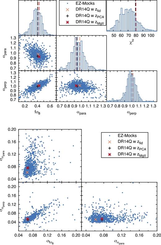
Same format as in Fig. 8, but for the full-AP fits, for the power-spectrum monopole, quadrupole, and hexadecapole. Unlike for the ε = 0 case of Fig. 8, for the full-AP case with the monopole, quadrupole, and hexadecapole are considered. The main values drawn from the different redshift estimates of the DR14Q data set (top panels) agree very well among themselves and represent a typical single example from the mocks. On the error panels (bottom panels), the data sets corresponding to the three redshift estimates present a typical behaviour with respect to the mocks.
As a summary, the observed shifts due to redshift failures are totally negligible for both the P(0) + P(2) and P(0) + P(2) + P(4) cases. The systematic shifts produced by fibre collisions on the P(0) + P(2) case are ≲ 0.01 for α∥, α⊥, and fσ8. Finally, the systematic shifts produced by fibre collisions when the hexadecapole is added are ∼0.02 for α∥ towards lower values, ∼0.01 for α⊥ towards higher values; and 0.027 on fσ8 towards higher values. These systematic shifts are below the statistical budget we expect from the data, given in the errors of the 〈xi〉 rows. However, we will add in quadrature these errors in Sections 6 and 7 when the covariances and cosmological results are presented.
We are also interested in testing the potential systematics of the theoretical modelling using full N-body mocks. We employ the same or-skycut mocks used in the section above, but now we perform a full-AP analysis on all three sets of mocks including the hexadecapole signal. The results are presented in Table 5 for the different satellite fractions, with and without the redshift smearing effect. When the fraction of satellite quasars is kept to 0, the |$f_{\rm no\text{-}sat}$| case, the systematic shifts observed for all the parameters are ≲ 0.01 for both with and without redshift smearing, and the model is able reproduce the expected signal. Introducing a satellite fraction produces some systematic shifts in some parameters. When the satellite fraction is kept to a value close to that used on the qpm mocks, fstd = 0.13, we observe shifts above 0.01 on all the parameters, which reaches deviations between 0.02 and 0.03 for all variables. When the fraction of satellites is high and no smearing is applied, the shifts on α∥ are ∼0.03, whereas on the rest of the cases are ≲ 0.02. We believe that these shifts are entirely due to a limitation of the theoretical model used to describe the clustering of quasars either by the adopted bias model or by the redshift space distortions. In this work, we do not investigate further the origin of these discrepancies, which in all cases are ≲ 1/3 of the expected statistical errors.
The top panel of Fig. 10 summarizes the systematic shifts of Table 5 along with the expected statistical errors (horizontal dashed lines) computed from the average errors of the 〈x〉i wcpwfoc row of ez mocks. For all the cases, the shifts are computed using the 〈xi〉 rows. The shifts obtained with the ez (dark blue) and qpm (light blue) mocks are driven by our treatment of observational inefficiencies with respect to their corresponding measured raw value. Therefore, these shifts display only the effects of fibre collisions and redshift failures on the measurements (any other systematic cancels). The effects are consistent among ez and qpm mocks, as expected, since they contain the same spectroscopic systematic effects. Examining the highest deviation on either ez or qpm mocks reveals that (i) for fσ8 the observational weights tend to produce a systematic shift towards higher values of 0.027; (ii) for α∥ these weights tend to reduce the measured quantity by 0.018; and (iii) for α⊥ the observational systematics tend to increase the measured quantity by 0.013. These values are summarized in Table 6 in the systematic observational budget column, σobs. The shifts obtained with the or-skycuts mocks and various satellite fractions, however, indicate modelling errors. We adopt as a systematic error the largest shift obtained with among the different satellite fractions and smearing effects, with respect to the true underlying value. Orange circle, red square, and green triangle symbols represent the results for |$f_{\rm no\text{-}sat}$|, fstd, and fhigh, respectively. The information in Fig. 10 does not display a clear correlation between the modelling systematic shift and the satellite fraction value. Although the true satellite fraction of the data is unknown, as a conservative choice we expect the upper limit to be less than fhigh, so we adopt the highest deviation among the six possible combinations as the modelling systematic contribution. These shifts are summarized in Table 6 under the modelling systematic column, σmod. As σobs and σmod are different sources of uncertainties, we add them in quadrature to our uncertainty budget |$\sigma ^2_{\rm systot}\equiv \sigma _{\rm obs}^2+\sigma _{\rm mod}^2$|. As both shifts tend to be of opposite signs and its origin is uncertain, we do not apply any shift to the best-fitting values of the measured quantities.
![Top panel: Systematic error shifts for fσ8, α∥, and α⊥ computed from the results presented in Table 5. The observational systematics represent the residual effects of the fibre collision + redshift failures. These shifts are computed as, [Δx]obs ≡ 〈xi〉 wcpwfoc − 〈xi〉 raw on both the ez and qpm mocks, as indicated; both sets have consistent systematic offsets. The modelling systematic results are computed only from the or-skycut mocks and they represent the uncertainties when recovering the true cosmological parameters due only to modelling limitations, [Δx]mod ≡ 〈xi〉 − xtrue. The different colours and symbols represent the satellite fractions, $f_{\rm no\text{-}sat}$, fstd, and fhigh for orange circles, red triangles, and green squares, respectively. The dashed black horizontal lines represent the expected statistical error for the data, computed as the average errors over the ez mocks. Bottom panel: The quantities of the top panel plotted as a function of the maximum k-wavenumber chosen to perform the fit. For simplicity, we only show the or-skycut mocks with smearing and we do not display the qpm mock results. The same colour code displayed in the top panel is used. Note that for the or-skycut mocks we display the deviation with respect to their expected value, whereas for the ez mocks the deviation is plotted with respect to the ‘raw’ case.](https://oup.silverchair-cdn.com/oup/backfile/Content_public/Journal/mnras/477/2/10.1093_mnras_sty453/2/m_sty453fig10.jpeg?Expires=1716429279&Signature=g3JjO-~ibcgiVgxidMA15ue6ohLf1qoMkJ4CzmewvWxBuGPsmQcF1x~VAu3~1f8HfFItPWyMxWR0W0vcY3bxd6jw6oyPUXRrOquLFtQXAtqXfauzk4Oj0gTIKW3keD8-t64FrBnJ3TYijzMOkjT4A7LYl7-mIuGzHGR3mLQi7qNdf5Fb0CywGvTyYH76z7EjOc-XBmIg3oAlXmIvelWdyFeD4mbq-u-YDCU4cXpJMMxZY~jUy9ym9G7zj-RJ7EVwYPS78xXffg8XscBLN8cZuwJRREVEjpse0tJOxr6RDwrvwvRUY7~AwQ5V~Q9d9kSjon4Ur3yLTqWmrJaA4qMH7w__&Key-Pair-Id=APKAIE5G5CRDK6RD3PGA)
Top panel: Systematic error shifts for fσ8, α∥, and α⊥ computed from the results presented in Table 5. The observational systematics represent the residual effects of the fibre collision + redshift failures. These shifts are computed as, [Δx]obs ≡ 〈xi〉 wcpwfoc − 〈xi〉 raw on both the ez and qpm mocks, as indicated; both sets have consistent systematic offsets. The modelling systematic results are computed only from the or-skycut mocks and they represent the uncertainties when recovering the true cosmological parameters due only to modelling limitations, [Δx]mod ≡ 〈xi〉 − xtrue. The different colours and symbols represent the satellite fractions, |$f_{\rm no\text{-}sat}$|, fstd, and fhigh for orange circles, red triangles, and green squares, respectively. The dashed black horizontal lines represent the expected statistical error for the data, computed as the average errors over the ez mocks. Bottom panel: The quantities of the top panel plotted as a function of the maximum k-wavenumber chosen to perform the fit. For simplicity, we only show the or-skycut mocks with smearing and we do not display the qpm mock results. The same colour code displayed in the top panel is used. Note that for the or-skycut mocks we display the deviation with respect to their expected value, whereas for the ez mocks the deviation is plotted with respect to the ‘raw’ case.
Total systematic error budget associated with the cosmological parameters, fσ8, α∥, and α⊥ computed from the results of Table 5 and Fig. 10. The sign and magnitude represent the over- or underestimated shift of the highest observed case, ez and qpm mocks for the observational systematics, and satellite fraction with and without smearing for the modelling systematics. Both contributions are added in quadrature, |$\sigma _{\rm systot}^2\equiv \sigma _{\rm obs}^2+\sigma _{\rm mod}^2$|, in order to produce a total systematic contribution that is added to the diagonal component of the covariance matrix of the data.
| σobs × 102 | σmod × 102 | |$\sigma _{\rm sys tot}^2\times 10^{3}$| | |
|---|---|---|---|
| fσ8 | +2.74 | −2.91 | 1.598 |
| α∥ | −2.12 | −3.09 | 1.404 |
| α⊥ | +1.36 | −2.35 | 0.737 |
| σobs × 102 | σmod × 102 | |$\sigma _{\rm sys tot}^2\times 10^{3}$| | |
|---|---|---|---|
| fσ8 | +2.74 | −2.91 | 1.598 |
| α∥ | −2.12 | −3.09 | 1.404 |
| α⊥ | +1.36 | −2.35 | 0.737 |
In addition, the bottom panel of Fig. 10 displays the same quantities of the top panel as a function of the maximum wavenumber used for the fit, kmax. For simplicity, we only show the results for the ez and or-skycut mocks with smearing. The systematic shifts reported in the top panel and Table 6 do not present any significant dependence with kmax, except for the extreme case of kmax = 0.37 h Mpc−1, which is outside the range of validity of the theoretical modelling at this redshift.
5.3 Isotropic fits on data
As an additional sanity check on our analysis procedure we perform a set of fits on the actual DR14Q data set changing different specifications in order to examine how strong the results are with respect to the data parametrization. For simplicity, we only perform these fits fixing ε to 0. We call the ‘standard’ (std) choice of specifications: (i) zfid as redshift estimates, (ii) the power-spectrum monopole and quadrupole as observables, (iii) of both NGC and SGC regions, (iv) sampled with a linear binning of Δk = 0.01 with k-centres at ki = (i + 0.5)Δk, (v) scale range considered between 0.02 ≤ k [h Mpc−1] ≤ 0.30, (vi) where the fibre collisions and redshift failures are corrected through wcpwfoc, and (vii) where the covariance matrix of the power-spectrum multipoles is inferred from 1000 ez mocks.
Table 7 and Fig. 11 display the measured fσ8, αiso, and b1σ8 measurements when some of these seven conditions are relaxed or modified. The +1/4, +2/4, and +3/4 rows correspond to the effect of shifting the centres of the k-bins by the respective fraction (with respect to the standard k-bin centre positions), and the ‘comb’ rows correspond to the result of combining these four results into a single measurement.10 Hereafter, we will refer to the ‘standard’ specification with the 4 k-bin centres combined as ‘comb’ or ‘combined’. Likewise, we refer to |$z_{\rm Mg\, {\small II}}$|-comb and zPCA-comb as the ‘combined’ specification with the redshift estimate changed from the fiducial case to the |$z_{\rm Mg\, {\small II}}$| and zPCA cases, respectively. The horizontal dashed lines in Fig. 11 correspond to the ±1σ errors of the ‘comb’ case. Along with the fiducial combined case, we present the combined measurements for the two other redshift estimates, |$z_{\rm Mg\, {\small II}}$| and zPCA. The NGC and SGC rows correspond to the measurements when only one Galactic Cap is used. Those rows labelled with log k correspond to changing the linear binning to logarithmic binning in the same k-range and with similar number of k-bins. Consequently, the log k cases have more k-measurements at large scales (low k-values) with respect the linear binning (and the covariance accounts for an extra statistical correlation because of this effect). The qpm row displays the result when the covariance matrix is changed by that inferred by the 400 realizations of the qpm mocks. For comparison, the results inferred from only 400 realizations of the ez mocks is also displayed. Finally, the effect of changing or turning off the imaging and spectroscopic weights is also presented. Bear in mind that all the results are highly correlated, as they are based on an identical data set, with the exception of those NGC and SGC cases, which can be considered as totally uncorrelated.
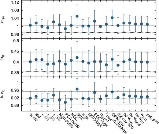
Impact of different parameters (see the text for definitions) on the measured b1σ8, fσ8, and αiso quantities, corresponding to those results presented in Fig. 7. For reference, the horizontal dashed lines correspond to the fiducial choice of parameters when the different k-bin centres results have been combined (comb option), and the horizontal dotted lines to the 1σ deviation for the same case.
Impact of different parameters (see the text for definitions) on the values of the DR14Q data set measurements: b1σ8, fσ8, and αiso, where the fits have been performed keeping ε = 0. The parameter which has the largest impact is the choice of covariance. The qpm covariance matrix shifts by 0.67σ the values of b1σ8 and αiso with respect to the ‘std’ case. However, further studies demonstrate that |${\sim }14\hbox{ per cent}$| of the mocks present such behaviour when the covariance matrix is changed from qpm- to ez-derived one. The SGC row also contains a 1σ shift, but in this case, the information content is significantly independent, as the std case contains more area than SGC, and therefore such ∼1σ shift is expected. For all cases, the mean value between the ±1σ edges is reported. The reported errors only represent the statistical error budget. Fig. 11 displays the values of this table.
| Case | b1σ8 | fσ8 | αiso | χ2/d.o.f |
|---|---|---|---|---|
| std | 0.928 ± 0.037 | 0.411 ± 0.047 | 1.017 ± 0.039 | 49/(56 − 6) |
| std +1/4 | 0.907 ± 0.034 | 0.411 ± 0.046 | 1.000 ± 0.035 | 51/(56 − 6) |
| std +2/4 | 0.908 ± 0.034 | 0.390 ± 0.045 | 0.994 ± 0.034 | 43/(56 − 6) |
| std +3/4 | 0.934 ± 0.035 | 0.392 ± 0.045 | 1.023 ± 0.035 | 47/(56 − 6) |
| std comb. | 0.918 ± 0.035 | 0.401 ± 0.046 | 1.006 ± 0.036 | 47/(56 − 6) |
| |$z_{\rm Mg\, {\small II}}$| comb. | 0.908 ± 0.045 | 0.404 ± 0.052 | 1.009 ± 0.050 | 48/(56 − 6) |
| zPCA comb. | 0.896 ± 0.037 | 0.390 ± 0.045 | 0.989 ± 0.038 | 45/(56 − 6) |
| NGC | 0.913 ± 0.044 | 0.408 ± 0.062 | 1.005 ± 0.046 | 41/(56 − 6) |
| SGC | 0.966 ± 0.055 | 0.421 ± 0.076 | 1.051 ± 0.056 | 42/(56 − 6) |
| logk | 0.918 ± 0.033 | 0.403 ± 0.044 | 1.002 ± 0.033 | 49/(54 − 6) |
| logk NGC | 0.915 ± 0.041 | 0.395 ± 0.060 | 1.002 ± 0.041 | 37/(54 − 6) |
| logk SGC | 0.948 ± 0.054 | 0.402 ± 0.073 | 1.026 ± 0.053 | 53/(54 − 6) |
| αiso = 1 | 0.914 ± 0.018 | 0.402 ± 0.041 | 1 | 49/(56 − 5) |
| kmax = 0.20 h Mpc−1 | 0.931 ± 0.045 | 0.387 ± 0.049 | 1.011 ± 0.040 | 34/(36 − 6) |
| qpm cov | 0.951 ± 0.037 | 0.413 ± 0.047 | 1.043 ± 0.039 | 46/(54 − 6) |
| ez cov 400 real. | 0.921 ± 0.039 | 0.385 ± 0.045 | 1.005 ± 0.040 | 43/(54 − 6) |
| no wsys | 0.936 ± 0.039 | 0.401 ± 0.047 | 1.017 ± 0.041 | 46/(56 − 6) |
| no wfoc | 0.929 ± 0.037 | 0.411 ± 0.047 | 1.017 ± 0.039 | 49/(56 − 6) |
| no wcp | 0.928 ± 0.036 | 0.401 ± 0.046 | 1.012 ± 0.037 | 48/(56 − 6) |
| wnoz | 0.924 ± 0.038 | 0.400 ± 0.046 | 1.013 ± 0.039 | 43/(56 − 6) |
| fid + P(4) | 0.926 ± 0.038 | 0.399 ± 0.045 | 1.011 ± 0.039 | 84/(84 − 6) |
We observe a ∼1σ deviation between NGC and SGC on the αiso and b1σ8 (both parameters are strongly correlated as is shown in Fig. 8), but since these two regions are statistically independent a 1σ shift is expected. The higher value of b1σ8 in the SGC is related to the observed excess of power in the power-spectrum monopole that is visible on top panel of Fig. 6. As stated previously, we conclude that this shift is not statistically significant.
For the rest of parameters studied, none have a strong effect on the cosmological parameters, with the exception of the redshift estimates (which we have already commented above) and the qpm covariance matrix, which produce a ∼1σ shift on b1σ8 and αiso, but no significant effect on fσ8. However, this 1σ shift appears only when we compare the ‘comb’ results with the qpm-cov results, which is drawn from the same k-bin centre condition as in ‘std’ case. Therefore, a fair comparison between ‘std’ and qpm-cov case yields only a 0.67σ offset. Further investigation on the potential impact of the choice of the covariance matrix suggests that this 0.67σ shift is not caused by the limited amount of realizations (400 on qpm versus 1000 on the ez mocks) nor by the differences in their off-diagonal elements that are sub-dominant in the total χ2 contribution. Therefore, the origin of this shift is located in the diagonal elements of the covariance, which present variations from 5–|$10\hbox{ per cent}$|.
Fig. D2 shows the ratio between the diagonal errors of ez and qpm mocks. In general, qpm-derived errors are |$5\hbox{ per cent}$| larger than ez-derived errors, but for the monopole at large scales, this tendency is inverted. Examining at the shifts on the ez mocks results presented in Table 4 when the ez- and qpm-derived covariances were applied, we find that 134/96211 of the mocks have shifts >0.67σ on αiso when the covariance matrix is changed, 75 towards lower values and 59 towards higher values, and consequently the average mean value of the inferred αiso is not significantly affected by the choice of the covariance (see Table 4). We conclude that the observed behaviour on the data is consistent with the behaviour of the mocks (occurs 14 per cent of times on the mocks) and that the origin of this effect is the 5–|$10\hbox{ per cent}$| differences in the diagonal terms of the two covariances, which in combination with the intrinsic statistical noise of the data can produce the observed ∼0.67σ fluctuation. In any case, we believe that the ez mocks are a better representation of the actual DR14Q data set, as they have been produced using different epoch snapshots, whereas the qpm is generated from a single one. Therefore, we assign a higher level of likelihood to those results derived from the ez-mock covariance, over those from the qpm.
We conclude that none of the studied specifications produce major systematic shifts in the studied parameters, and we consider that our results are robust under the change of the specifications presented in this section.
6 RESULTS
In this section, we describe the results on the DR14Q data sample. We present the results for both isotropic fits (keeping ε = 0) and full-AP fits. Additionally, we perform two parallel analyses, (i) we consider the full 0.8 ≤ z ≤ 2.2 redshift range as a single redshift bin, (ii) we divide this redshift range into three overlapping redshift bins, as described above in Section 4.2.
6.1 Isotropic fits
We start by performing an isotropic fit to the power-spectrum monopole and quadrupole of the DR14Q data set, keeping ε = 0. Here, we do not consider to use the hexadecapole because, as demonstrated in Section 5.1, it does not add any extra information when ε is set to a constant value. Table 8 displays the mean value between the 1σ errors, xmean ≡ [(xbf + σ+) + (xbf − σ−)]/212 for the free parameters of the model. The different columns display the results using the fiducial redshift estimate, zfid, applied to the individual NGC and SGC, along with the combination of both. In addition, the results for the two extra redshift estimates, |$z_{\rm Mg\, {\small II}}$| and zPCA are presented. For all the cases, the rest of the specifications correspond to the ‘standard’ case defined in Section 5.3, unless otherwise stated. Fig. 8 has previously shown the results on the three redshift estimates corresponding to the entire NGC+SGC sample for the parameters b1σ8, fσ8, and αiso, along with the ez mocks. As described in Section 5.3, the results of the NGC and SGC are consistent within 1σ for all the parameters. The results on the different redshift estimates are also consistent and there is no observed evident tension in any of the parameters. The errors associated with the parameters inferred from the |$z_{\rm Mg\, {\small II}}$| redshifts are in general higher, as already discussed in Section 5.1.
Inferred parameters of the model for the isotropic fit (ε = 0) when the power-spectrum monopole and quadrupole are used. We report the results for the DR14Q data set for a fiducial redshift estimate, zfid, along with two additional redshift estimates, |$z_{\rm Mg\, {\small II}}$| and zPCA. For the zfid case, we present the results of fitting the NGC and SGC independently. For all cases, the ez-derived covariance is used. The rest of specifications are fixed to the ‘standard’ choice (see the definition in Section 5.3). The units of σP are [h−1 Mpc]. The errors shown only represent the statistical error budget. For all parameters, we report the mean value between the 1σ errors, xmean ≡ [(xbf + σ+) + (xbf − σ−)]/2.
| zfid | zfid (NGC) | zfid (SGC) | |$z_{\rm Mg\, {\small II}}$| | zPCA | |
|---|---|---|---|---|---|
| b1σ8 | 0.928 ± 0.037 | 0.913 ± 0.044 | 0.966 ± 0.055 | 0.933 ± 0.049 | 0.909 ± 0.039 |
| fσ8 | 0.411 ± 0.047 | 0.408 ± 0.062 | 0.421 ± 0.076 | 0.414 ± 0.055 | 0.393 ± 0.046 |
| αiso | 1.017 ± 0.039 | 1.005 ± 0.046 | 1.051 ± 0.056 | 1.034 ± 0.055 | 1.003 ± 0.041 |
| b2σ8 | 0.60 ± 0.57 | 0.75 ± 0.63 | −0.24 ± 1.13 | 0.20 ± 0.72 | 0.58 ± 0.53 |
| σP | 5.20 ± 0.42 | 5.54 ± 0.58 | 4.75 ± 0.77 | 5.30 ± 0.52 | 4.98 ± 0.42 |
| Anoise | 7.2 ± 2.3 | 6.0 ± 3.3 | 8.1 ± 7.3 | 5.4 ± 3.8 | 4.6 ± 2.6 |
| χ2/d.o.f | 49/(56 − 6) | 41/(56 − 6) | 42/(56 − 6) | 48/(56 − 6) | 43/(56 − 6) |
These results are affected by the prior condition of ε = 0. These results imply that H(z)DA(z) is equal to |$H^{\rm fid}(z)D_A^{\rm fid}(z)$|, which is similar to the best-fitting Planck cosmology. Therefore, the isotropic derived results are not independent from Planck results, and thus, Planck-cosmic microwave background (CMB) data should not be added to these results as an extra uncorrelated data set.
6.2 Anisotropic fits
We consider the power-spectrum monopole, quadrupole, and hexadecapole, and perform a full-AP fit, relaxing the ε = 0 condition of the previous section. Thus, α∥ and α⊥ can freely vary, which enable constraints to be placed on H(z)rs(zd) and DA(z)/rs(zd) independent of the CMB data.13 Table 9 displays these results using the same notation as in Table 8. The first three columns show the results for the different redshift estimates when only the power-spectrum monopole and quadrupole have been fitted. The following three columns present the results when the power-spectrum hexadecapole is added to the analysis. For all the cases, we fix the rest of specifications to ‘combined’, as they are described in Section 5.3, which consist on the ‘standard’ specifications combining the four shifts on the k-bin centres.
Parameters of the model for the full-AP fit. We report the results for the DR14Q data set for a fiducial redshift estimate, zfid, along with two extra redshift estimates, |$z_{\rm Mg\, {\small II}}$| and zPCA. The first three columns correspond to the results when the power-spectrum monopole and quadrupole are used; the three following columns are produced when the power-spectrum hexadecapole is added to the analysis. For all cases, the ez-derived covariance is used, and the rest of specifications correspond to ‘comb’ as described in Section 5.3. The units of σP are [Mpc h−1]. The errors shown only represent the statistical error budget.
| zfid | |$z_{\rm Mg\, {\small II}}$| | zPCA | zfid + P(4) | |$z_{\rm Mg\, {\small II}}+P^{(4)}$| | zPCA + P(4) | |
|---|---|---|---|---|---|---|
| b1σ8 | 0.930 ± 0.041 | 0.965 ± 0.059 | 0.941 ± 0.059 | 0.908 ± 0.038 | 0.859 ± 0.049 | 0.871 ± 0.046 |
| fσ8 | 0.366 ± 0.072 | 0.329 ± 0.083 | 0.314 ± 0.079 | 0.412 ± 0.064 | 0.427 ± 0.065 | 0.404 ± 0.066 |
| α∥ | 1.040 ± 0.089 | 1.17 ± 0.12 | 1.13 ± 0.11 | 0.976 ± 0.062 | 0.919 ± 0.076 | 0.937 ± 0.076 |
| α⊥ | 0.977 ± 0.056 | 0.953 ± 0.063 | 0.941 ± 0.054 | 1.015 ± 0.052 | 1.011 ± 0.055 | 0.994 ± 0.050 |
| b2σ8 | 0.49 ± 0.58 | −0.21 ± 0.65 | 0.33 ± 0.55 | 0.56 ± 0.55 | 0.51 ± 0.65 | 0.61 ± 0.52 |
| σP | 5.18 ± 0.49 | 5.73 ± 0.95 | 5.22 ± 0.65 | 4.98 ± 0.41 | 5.05 ± 0.46 | 4.75 ± 0.40 |
| Anoise | 6.8 ± 3.5 | 2.2 ± 4.5 | 3.8 ± 3.2 | 6.5 ± 2.7 | 4.2 ± 2.9 | 3.7 ± 2.5 |
| χ2/d.o.f | 47/(56 − 7) | 47/(56 − 7) | 43/(56 − 7) | 81/(84 − 7) | 80/(84 − 7) | 81/(84 − 7) |
The performance of the model corresponding to column zfid + P(4) was previously displayed in the top panel of Fig. 5 for the full NGC+SGC data set along with the DR14Q measurements. Likewise, Fig. 9 presents the results from the different +P(4) columns along with the results from the ez mocks for the parameters of cosmological interest, fσ8, α∥, and α⊥.
When the power-spectrum hexadecapole is added to the analysis some parameters shift their value at the 1σ level. When adding the hexadecapole signal we are introducing 28 new data points (to the 56 already from monopole and quadrupole), which are highly independent, as indicated by the off-diagonal terms of the covariance matrices in Fig. D1. We investigate the significance of those shifts using the ez mocks. The top panel of Fig. 12 displays the quantity Δx ≡ xMQ − xMQH, where xMQ is the variable estimated from the monopole and quadrupole measurement, and xMQH is the value when the hexadecapole is added. The bottom panel shows the same information but for the errors of the x-corresponding quantity. From the top panel, the shifts presented by the results for the zfid redshift estimate (orange symbols) are typical with respect to the observed shifts of the mocks for the three variables of interest. For the |$z_{\rm Mg\, {\small II}}$| and zPCA cases, however, the shifts on α∥ deviate by 2σ from the expected behaviour of the mocks, although they are along the degeneracy region among the studied parameters. Certainly, the discrepancy among the different redshift estimates is larger when only the monopole and quadrupole are considered, as the values of α∥ estimated from |$z_{\rm Mg\, {\small II}}$| and zPCA are about 1σ from the value obtained with zfid. Adding the hexadecapole produces more consistent results among the three redshift estimators, as shown in Fig. 9. The bottom panel of Fig. 12 reveals that the reduction on the errors obtained by adding the hexadecapole are typical with respect to the behaviour observed by the mocks.
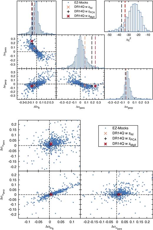
Top panel: Difference between the best-fitting value of the mocks (blue symbols) and the DR14Q data (different colour symbols for the different redshift estimates) when only the monopole and quadrupole are used, xMQ, and when the hexadecapole is added, xMQH, for the different cosmological parameters: Δx ≡ xMQ − xMQH. Bottom panel: The same format as the top panel but for the error associated with the each parameter, σx, |$\Delta \sigma _x\equiv \sigma _{x^{\rm MQ}}-\sigma _{x^{\rm MQH}}$|. On average, the expected shift on Δx should be 0 if no extra systematic is added by the hexadecapole. However, from Table 5, we know that adding the hexadecapole produces a systematic shift of −0.02 on α∥ and +0.01 on α⊥, which slightly shifts the centre of the measurements from the black dashed lines. We expect the hexadecapole to reduce the errors on the measured quantities (on average) and therefore |$\sigma _x^{\rm MQH}<\sigma _x^{\rm MQ}$|, which shifts the centre of the Δσx distribution towards the positive quadrant for all the variables.
Fig. 13 presents a further comparison among the different cases presented in Table 9 via 2D contour plots of the cosmological parameters of interest. All the measurements are made using 20 mcmc chains with half a million of steps each. For the case of monopole and quadrupole, a flat prior between 0.5 and 1.5 on α∥ and α⊥ is set to speed the convergence. Outside these ranges a ∼x2 function is added to the χ2, where x is the difference between the studied parameter (in this case α∥ and α⊥) and the limit of the prior (in this case 0.5 and 1.5). This condition correspond to flat priors within the range 15.83 ≤ H(z)rs(zd)[103 km s−1] ≤ 47.5 and 6.07 ≤ DA(z)/rs(zd) ≤ 18.22. For H(z)rs(zd) < 15.83 × 10³ km s−1, the prior is the responsible of the abrupt change in the shape of the likelihood function.
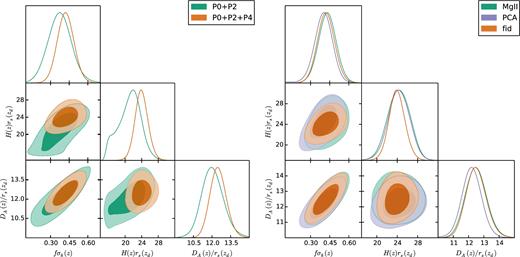
Posterior likelihood contours from the DR14Q data in the redshift range 0.8 ≤ z ≤ 2.2 for the fσ8, DA/rs, and Hrs cosmological parameters derived from the mcmc chains. The left-hand panels display the results when the power-spectrum monopole and quadrupole are used (green contours), and when the hexadecapole signal is added (orange contours). The right-hand panel shows the comparison for different redshift estimates, zfid (in orange), |$z_{\rm Mg\, {\small II}}$| (in green) and zPCA (in violet contours), for the power-spectrum monopole, quadrupole, and hexadecapole. When the power-spectrum monopole and quadrupole are used alone (green contours on the left-hand panel), we use a flat prior between 0.5 and 1.5 on the scale dilation factors, α∥ and α⊥, in order to improve the convergence of the chains. The units of H(z)rs(zd) are 103 km s−1.
The left-hand panel shows the comparison among DA(z)/rs(zd), H(z)rs(zd), and fσ8 for the redshift estimate, zfid when the power-spectrum monopole and quadrupole is used (green contours), and when the hexadecapole is added (orange contours). The information contained by the hexadecapole improves the constraint on H(z)rs(zd) and consequently breaks the degeneracy between H(z)rs(zd) and the other two parameters. The right-hand panel we show the constraints on the same variables for the case where the three multipoles are used, but now under different redshift estimates: zfid as before in orange contours, |$z_{\rm Mg\, {\small II}}$| in green and zPCA in purple contours. In summary, we obtain a good agreement among the different redshift estimates when the three power-spectrum multipoles are used, which strongly supports the idea that the results are not significantly affected by the choice of the automated redshift classification. However, we believe that zfid is the best procedure of obtaining the redshifts and we adopt those as the main results of this paper.
The marginalized errors for the cosmological parameters that contain the full error budget are fσ8(1.52) = 0.420 ± 0.076 and DA(1.52)/rs(zd) = 12.48 ± 0.71 and H(1.52)rs(zd) = [24.0 ± 1.8] × 103 km s−1 with a correlation coefficient of |$\rho _{[f\sigma _8-D_A/r_s]}=0.74$|, |$\rho _{[f\sigma _8-Hr_s]}=0.40$| and |$\rho _{[D_A/r_s-Hr_s]}=0.16$|
In Section 7, we will explore the cosmological constraints drawn from these results.
6.3 Multiple redshift bins
We perform a parallel analysis to that presented in the above Section 6.2, re-doing the full-AP fits in three overlapping redshift bins. We refer to them as lowz: 0.8 ≤ z ≤ 1.5 with effective redshift of zlowz = 1.19; midz 1.2 ≤ z ≤ 1.8 with effective redshift of zmidz = 1.50; and highz 1.5 ≤ z ≤ 2.2 with effective redshift zhighz = 1.83. Table 10 displays the best-fitting results for these three redshift bins. The measurements and best-fitting models were also given in Fig. 7 and briefly discussed in Section 4.2. The approach of dividing the full redshift range into overlapping redshift bins is complementary to the single broad redshift bin analysis presented above. Although some large-scale signal is lost when dividing the sample, the three redshift bin analysis has the advantage of capturing the redshift evolution of parameters, such as the structure growth factor or the galaxy bias. In the following section, we will compare the multiple z-bin approach with the single z-bin, showing the different power when constraining cosmological parameters. An alternative approach for analysing redshift-dependent quantities without sub-dividing the full redshift range was proposed by Zhu, Padmanabhan & White (2015) and developed specifically for redshift space distortions in Ruggeri et al. (2017b). Also in Ruggeri et al. (2017a), this technique was tested on the DR14Q ez mocks and it is presented for the same DR14Q data set in the companion papers Ruggeri et al. (2018) and Zhao et al. (2018).
Parameters of the model for the full AP fit when the DR14Q 0.8 ≤ z ≤ 2.2 sample is divided in three overlapping redshift bins. We report the results for a fiducial redshift estimate, zfid for the NGC+SGC sample. The results of the midz sample correspond to the vetoed sample (see the text). For all cases, we used the ez-derived covariance and the ‘standard’ specifications corresponding to the definition in Section 5.3. The correlation among the different parameters are presented in Fig. 14. The units of σP are [Mpc h−1]. The errors shown only represent the statistical error budget.
| N+S (zfid) | 0.8 ≤ z ≤ 1.5 | 1.2 ≤ z ≤ 1.8 | 1.5 ≤ z ≤ 2.2 |
|---|---|---|---|
| b1σ8 | 0.900 ± 0.056 | 0.945 ± 0.059 | 0.947 ± 0.077 |
| fσ8 | 0.440 ± 0.087 | 0.364 ± 0.093 | 0.468 ± 0.091 |
| α∥ | 0.994 ± 0.075 | 1.05 ± 0.12 | 0.98 ± 0.13 |
| α⊥ | 1.027 ± 0.075 | 1.014 ± 0.069 | 1.039 ± 0.067 |
| b2σ8 | 0.66 ± 0.85 | 0.71 ± 0.60 | 0.87 ± 0.55 |
| σP | 4.11 ± 0.58 | 5.25 ± 0.68 | 6.38 ± 0.77 |
| Anoise | 9.7 ± 5.6 | 7.8 ± 4.0 | 4.4 ± 3.3 |
| χ2/d.o.f | 71/(84 − 7) | 91/(82 − 7) | 99/(84 − 7) |
The first fit to the midz redshift bin produced a high value of χ2, 122/(84 − 7), which is a more than 3σ fluctuation, and none of the studied mocks have such high |$\chi _{\rm min}^2$| (the highest value for the best-fitting χ2 from the mocks on the midz redshift bin is 107) when they are analysed in the same manner as the DR14Q data set. Examining Fig. 7 (purple symbols for midz redshift bin), reveals that the origin of this high χ2 is two >3σ outliers, one in the quadrupole (3.2σ offset), the second one in the hexadecapole (4σ offset) at k ≃ 0.11 h Mpc−1. Although one outlier at ∼3σ is expected given the number of degrees of freedom (84 − 7), two >3σ offsets are very unlikely (|$<{}0.1\hbox{ per cent}$|). We believe that such deviations are caused by an uncorrected observational systematic of unknown origin. We have checked the shape of the hexadecapole for the two extra redshift estimates, and both present these two features at similar significance 3.2σ and 3.6σ for the |$z_{\rm Mg\, {\small II}}$| and zPCA redshifts estimates, respectively. Therefore, using a different redshift estimate does not modify the high χ2 issue (|$\chi ^2_{\rm PCA}=107$| and |$\chi ^2_{\rm Mg\, {\small II}}=103$|). We have also tested whether the smoothing of the n(z) distribution of the associated random catalogue could have an impact on these outliers, but observed no significant effect. We also have investigated these two features in the NGC and SGC patches separately. For example, the feature in the hexadecapole is equally present in the NGC and SGC patches, with measurements of |$P_{\rm NGC}^{(4)}(k=0.115\,h\,{\rm Mpc}^{-1})=-3444\pm 1608\,[h^{-1}\,{\rm Mpc}]^3$| and |$P_{\rm SGC}^{(4)}(k=0.115\,h\,{\rm Mpc}^{-1})=-5355\pm 2005\,[h^{-1}\,{\rm Mpc}]^3$|(and |$P_{\rm N+S}^{(4)}(k=0.115\,h\,{\rm Mpc}^{-1})=-5161\, \pm 1246[h^{-1}\,{\rm Mpc}]^3$| in the combined NGC+SGC sample), whereas the prediction from the mean of the 1000 realizations of the ez mocks is −116 ± 40 [h−1 Mpc]3. This result translates into a 2σ deviation for the NGC, and a 2.6σ deviation for the SGC, which are not particularly high if they are analysed individually. However, when both patches are combined, the fluctuation rises up to the reported 4σ. In the full-redshift range 0.8 ≤ z ≤ 2.2, such a systematic is probably diluted among the other two redshift bins, which reduces the tension between the model and the measurement, providing a consistent |$\chi _{\rm min}^2=81$| as reported in Table 9. In order to test the impact of these systematics in the parameters of the model, we remove these two frequencies in the corresponding multipole and redo the fitting process. After vetoing just these two >3σ outliers, the χ2 is reduced to 91, confirming that the origin of the high χ2 is produced by these frequencies at k ≃ 0.11 h Mpc−1. We check that the mean values of the model are not affected by more than 0.33σ statistical shifts, where fσ8 is the most affected parameter. We leave for a future work the study and characterization of this systematic effect. From this point, we proceed our analysis using the vetoed midz sample.
Table 10 displays the measurements of the cosmological parameters of interest for the different redshift bins. Some of these parameters indicate a redshift evolution across the three redshift bins. Of particular interest is σP, whose magnitude increases with redshift by 3σ. The σP parameter partially captures the uncertainty on the redshift estimation, as described before at the end of Section 2.3.1. Certainly, since the redshift error increases with redshift, σP necessarily has to increase as well. The other parameters have a negligible dependence with redshift, such as fσ8 and b1σ8. Although f(z) and b1(z) may have a strong increasing dependence with redshift, σ8(z) decreases with redshift, which counterbalances their effect. The quantities α∥ and α⊥ represent deviations with respect to a fiducial model that do change with redshift. Therefore, although we do not detect an explicit redshift dependence on these parameters, the fiducial model does change with redshift, and the cosmological information we obtained by having three measurements of DA/rs and Hrs instead of a single one is more interesting.
Since the midz redshift bin fully overlaps with lowz and highz, a large correlation among the different parameters is expected. Fig. 14 displays the correlation among the cosmological parameters fσ8(z), DA(z)/rs(zd), and H(z)rs(zd) computed from the ez mocks. We use these correlation factors to compute the off-diagonal coefficient terms across z-bins of the 9 × 9 covariance matrix of the data for the cosmological parameters fσ8(z), DA(z)/rs(zd), and H(z)rs(zd) at zlowz = 1.19, zmidz = 1.50, and zhighz = 1.83. For the off-diagonal coefficients terms belonging to the same z-bins, we keep the cross-correlation value obtained by the Gaussian approximation to the data, which is consistent with the one obtained with the mocks.
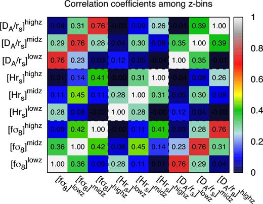
Cross-covariance for the lowz, midz, and highz redshifts bins for fσ8, Hrs, and DA/rs parameters derived from the mocks. The midz redshift bin fully overlaps with lowz and highz and therefore some correlation of parameters is expected. The typical cross-correlation factors are 0.3–0.4, in line with the fraction of overlapped volume. The lowz and highz data sets, however, are non-overlapping and therefore have small correlation (≪0.1) among their parameters.
As before, we present the results of this section in form of a data vector along with its covariance matrix. We run mcmc chains to the individual overlapping redshift bins, as was done in the previous sections. In this case, we set up different priors to avoid secondary minima at α∥ and α⊥ outside 0.8 ≤ α∥, ⊥ ≤ 1.2. These secondary minima arises as a consequence of having subsamples with smaller volumes compared to the single bin case. For example, we have identified a second minima in the highz sample, whose χ2 is |${\sim }\chi ^2_{\rm min}+2$|, and which is located at fσ8 ≃ 0.8 and α⊥ ≃ 1.4 (see Appendix E for further details). Table 11 summarizes the different priors set on the different samples.
Flat priors ranges set on the three redshift-bin samples on the AP dilation scales. The priors on the other parameters are the same than those described in Table 3.
| Sample | α∥-flat prior | α⊥-flat prior |
|---|---|---|
| 0.8 < z < 2.2 | [0.00, 2.00] | [0.00, 2.00] |
| lowz | [0.50, 1.50] | [0.50, 1.50] |
| midz | [0.65, 1.50] | [0.50, 1.50] |
| highz | [0.70, 1.70] | [0.80, 1.20] |
| Sample | α∥-flat prior | α⊥-flat prior |
|---|---|---|
| 0.8 < z < 2.2 | [0.00, 2.00] | [0.00, 2.00] |
| lowz | [0.50, 1.50] | [0.50, 1.50] |
| midz | [0.65, 1.50] | [0.50, 1.50] |
| highz | [0.70, 1.70] | [0.80, 1.20] |
The resulting data vector taking the mcmc steps whose |$\chi ^2\le \chi ^2_{\rm min}+14.16$| along with the corresponding 9 × 9 covariance matrix is presented in Table 12. The covariance is constructed using the diagonal terms, as well as the off-diagonal terms belonging to same redshift bin, extracted from the mcmc chains computed at the three redshift bins using the same criteria described for the data vector, combined with the cross-correlation coefficients from different redshift bins derived from the mocks and presented in Fig. 14. The systematic error contribution is already included in the values of Table 6.
Data vector and covariance matrix elements for the results derived from the three overlapping redshift bins lowz (L superindex), midz (M superindex), and highz (H superindex). The first row displays the data vector measurements, xi in the same units used on the data vector of equation (27). The second row displays the diagonal errors (with their systematic contribution), σi, of the covariance matrix corresponding to the data elements above. Below the cross-correlation among the data vector elements are presented.
| [fσ8]L | [fσ8]M | [fσ8]H | [Hrs]L | [Hrs]M | [Hrs]H | [DA/rs]L | [DA/rs]M | [DA/rs]H | |
|---|---|---|---|---|---|---|---|---|---|
| xi | 0.4736 | 0.3436 | 0.4998 | 19.6782 | 19.8637 | 26.7928 | 12.6621 | 12.4349 | 13.1305 |
| σi | 0.0992 | 0.1104 | 0.1111 | 1.5866 | 2.7187 | 3.5632 | 0.9876 | 1.0429 | 1.0465 |
| [fσ8]L | 1.0000 | 0.3563 | 0.0917 | 0.3156 | 0.1103 | 0.0081 | 0.7192 | 0.2882 | 0.0425 |
| [fσ8]M | − | 1.0000 | 0.4244 | 0.0820 | 0.5231 | 0.1388 | 0.2280 | 0.7446 | 0.3089 |
| [fσ8]H | − | − | 1.0000 | −0.0239 | 0.1083 | 0.2490 | 0.0323 | 0.2795 | 0.7954 |
| [Hrs]L | − | − | − | 1.0000 | 0.2836 | −0.0005 | 0.1024 | 0.0385 | −0.0304 |
| [Hrs]M | − | − | − | − | 1.0000 | 0.3144 | 0.0462 | 0.3462 | 0.0904 |
| [Hrs]H | − | − | − | − | − | 1.0000 | −0.0399 | 0.0819 | 0.0637 |
| [DA/rs]L | − | − | − | − | − | − | 1.0000 | 0.3490 | −0.0065 |
| [DA/rs]M | − | − | − | − | − | − | − | 1.0000 | 0.3890 |
| [DA/rs]H | − | − | − | − | − | − | − | − | 1.0000 |
Fig. 15 displays the full non-Gaussian posterior corresponding to the different redshift bins on the cosmological parameters of interest. The contours have been produced using the full set of mcmc chains and not the Gaussian approximation provided by Fig. 15 (see Appendix E for the differences between the actual likelihood posterior shape and its corresponding Gaussian approximation). In Fig. 17, we display these measurements as a function of redshift along with other probes.
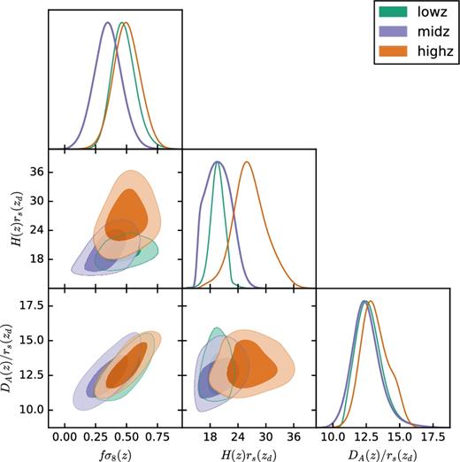
Posterior likelihood contours from the DR14Q data corresponding to the different redshift bins: lowz zeff = 1.19 (green contours); midz zeff = 1.50 (purple contours); zeff = 1.83 (orange contours); for fσ8, DA/rs, and Hrs derived from the mcmc chains. In all cases, the power-spectrum monopole, quadrupole, and hexadecapole have been used. In the case of the midz two k-wave numbers have been vetoed as described in the main text. The priors set on the different parameters are displayed in Table 11. The units of H(z)rs(zd) are 103 km s−1.
6.4 Bias evolution
In this section, we aim to compare the results on the measured linear bias of the quasars with previous measurements. Laurent et al. (2017) measured the quasar correlation function monopole on the redshift range 0.9 ≤ z ≤ 2.2 for the eBOSS DR13 quasar sample (Albareti et al. 2017) and obtained b1(z = 1.55) = 2.45 ± 0.05 when the full redshift range was considered as a single bin, and when the sample was divided in several redshift bins (see black symbols and lines of Fig. 16). In this paper, we have measured b1σ8(z) in a similar redshift range using the DR14 that contains ∼80 000 more quasars and approximately twice the DR13 effective volume. Simply taking the ratio of our b1σ8 measurement and the Planck cosmology prediction for σ8, |$\sigma _8^{\rm Planck}$| produces |$b_1\sigma _8(z)/\sigma _8^{\rm Planck}(z)\equiv b_1(z)$|. When the isotropic fit is performed (i.e. setting ε = 0) using the power-spectrum monopole and quadrupole measurements, b1(z = 1.52) = 2.30 ± 0.11, whereas the full-AP analysis using the three power-spectrum multipoles yields b1(z = 1.52) = 2.32 ± 0.10. Both results are consistent, demonstrating that the bias measurements and errors do not depend on the type of fit used, or whether the hexadecapole is added. Also, our results are in good agreement with those presented in Laurent et al. (2017). We believe that the reason our errors are larger than those from Laurent et al. (2017) is because we marginalize over a larger set of nuisance parameters, such as b2 and σP. Fig. 16 displays the measurements by Laurent et al. (2017) when they sub-divide the full redshift range in four non-overlapping redshift bins (black symbols) along with the best-fitting model as a function of redshift (solid black lines for the best-fitting model and dashed lines for 1σ confidence level). The coloured symbols display the measurements we report in this paper: purple symbols when the full redshift range is considered as a single bin and orange symbols when the redshift range is divided in the three previously mentioned redshift bins. The triangle symbols represent the measurements when the full-AP fits are performed, whereas the circle symbols indicate the isotropic fit. In all the cases, there is an excellent agreement among the two analyses, demonstrating the consistency among the DR13Q and DR14Q and the two bias models used.
![Coloured symbols display the measured linear bias parameter for the DR14Q sample, as a function of redshift when the function σ8(z) from Planck cosmology is assumed, b1(z) ≡ [b1σ8(z)]/σ8(z)Planck, where b1σ8(z) is the actual parameter measured in this paper. Orange symbols display the results when the DR14Q sample is divided in three overlapping redshift bins: lowz, midz, and highz. Purple symbols display the results when the full redshift range (0.8 ≤ z ≤ 2.2) is considered as a single bin. Circles display the results when b1σ8(z) is computed assuming ε = 0 (isotropic fit) and triangle symbols when this condition is relaxed (full-AP fit). Black empty symbols display the results found by Laurent et al. (2017) on the DR13Q sample using four different non-overlapping redshift bins, along with its best fit (solid black lines and dashed black lines for 1σ uncertainties). For the three overlapping redshift bins, the correlation parameters are (i) for the isotropic case, ρlow-mid = 0.42, ρlow-high = 0.04, ρmid-high = 0.42; (ii) for the full-AP case, ρlow-mid = 0.30, ρlow-high = −0.02, ρmid-high = 0.32.](https://oup.silverchair-cdn.com/oup/backfile/Content_public/Journal/mnras/477/2/10.1093_mnras_sty453/2/m_sty453fig16.jpeg?Expires=1716429279&Signature=4VPMAdCVlnES~MPLzo70uc5i9N10VawIRnVJSi2AYZeGdTkUc9czbDESDkD2-UG9bQ8FBaQbrvFn2aPi~Fpr9LV37zoBtDiX90EBJaDn0pL75mMsy-ZKhA5R3DKInub6D7F~dz1pGVwItb3UFYSLsmzZfZhfDFPgUfnJG~GiuKtTaIDl6IJ1ChGvnhgET1d4-8UQ3YujZ4r3F3Fj-7-BGD4uA9NnIQT9mZUggJ8sNAewPL88F0xqGvbngFLWbXSS1M8YQ-n1SZv029LnqE~p8nrc8MKEpJaB3b8GLwMh0wh0qoQCD25Muis0Sk4J5aKFci1lttGPX4Yq0faZrP7TzA__&Key-Pair-Id=APKAIE5G5CRDK6RD3PGA)
Coloured symbols display the measured linear bias parameter for the DR14Q sample, as a function of redshift when the function σ8(z) from Planck cosmology is assumed, b1(z) ≡ [b1σ8(z)]/σ8(z)Planck, where b1σ8(z) is the actual parameter measured in this paper. Orange symbols display the results when the DR14Q sample is divided in three overlapping redshift bins: lowz, midz, and highz. Purple symbols display the results when the full redshift range (0.8 ≤ z ≤ 2.2) is considered as a single bin. Circles display the results when b1σ8(z) is computed assuming ε = 0 (isotropic fit) and triangle symbols when this condition is relaxed (full-AP fit). Black empty symbols display the results found by Laurent et al. (2017) on the DR13Q sample using four different non-overlapping redshift bins, along with its best fit (solid black lines and dashed black lines for 1σ uncertainties). For the three overlapping redshift bins, the correlation parameters are (i) for the isotropic case, ρlow-mid = 0.42, ρlow-high = 0.04, ρmid-high = 0.42; (ii) for the full-AP case, ρlow-mid = 0.30, ρlow-high = −0.02, ρmid-high = 0.32.
7 COSMOLOGICAL IMPLICATIONS
In this section, we compare and combine our cosmological results with other probes such as the BOSS DR12 results (Alam et al. 2017; Bautista et al. 2017b; du Mas des Bourboux et al. 2017) and CMB constraints from Planck Collaboration et al. (2016).
The panels of Fig. 17 display the DR14Q measurement of fσ8, DA, and H in purple circles, where the empty symbols represent the three overlapping redshift bin measurements of Section 6.3, and the filled symbols the measurement considering the full range as a single redshift bin as described in Section 6.2. Along with these measurements, we display the RSD results from the Main Galaxy Sample (MGS) DR7 SDSS-II (Howlett et al. 2015), the BOSS LRGs DR12 SDSS-III consensus results derived from RSD and BAO analyses (Ata et al. 2018); and the measurement from the BOSS Ly α DR12 SDSS-III auto- and cross-correlation result derived from BAO-only analyses (Bautista et al. 2017b; du Mas des Bourboux et al. 2017). The black dashed line along with the green bands areas represents the ΛCDM-Planck prediction when a flat Universe is assumed (Planck Collaboration et al. 2016). The DR14Q measurements cover the, currently, unexplored region (in terms of fσ8, H, and DA measurements) between redshifts 1 and 2, and are in fairly good agreement with the predictions from Planck.
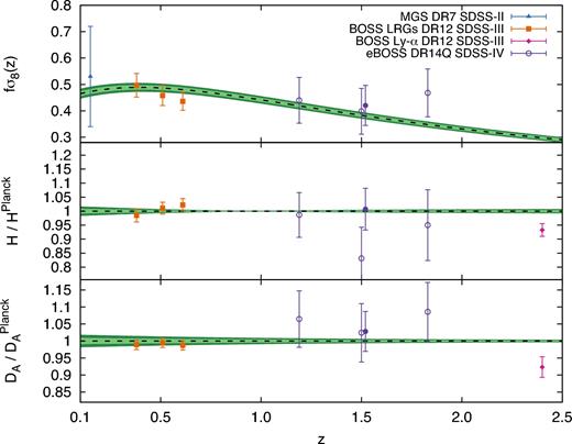
The three panels show the redshift dependence of fσ8, H, and DA inferred from a number of SDSS galaxy and quasar surveys. The black dashed lines along with the green bands display the predictions assuming a flat-ΛCDM Planck cosmology (Planck Collaboration et al. 2016). The blue triangle represents the RSD analysis of the SDSS-II MGS DR7 at zeff = 0.15 (Howlett et al. 2015); the orange squares display the BAO and RSD analyses from SDSS-III BOSS DR12 LRGs (Alam et al. 2017) in the range 0.15 ≤ z ≤ 0.75; the magenta symbols represent the SDSS-III Ly α measurement at zeff = 2.4 from the auto- and cross-correlation analyses (Bautista et al. 2017b; du Mas des Bourboux et al. 2017). The results derived from DR14Q SDSS-IV (this work) are represented by the purple symbols, where the filled symbols indicate the measurements from a single-redshift bin analysis at zeff = 1.52, and the empty symbols from the three overlapping redshift bins at zeff = 1.19, zeff = 1.50, and zeff = 1.83. For clarity, the DA and H quantities have been normalized to the fiducial prediction by the ΛCDM Planck cosmology.
The methodology used to derive the cosmological parameters of this paper (as well as those of BOSS DR12) assumes General Relativity (GR) as the theory of gravity. In a ΛCDM scenario, we relate the parameter for the growth of structure, f, with the matter density of the Universe, Ωm, through the parametrization, f(z) = Ωm(z)γ (Kaiser 1987; Linder 2005), where γ is the growth index; for GR γ = 0.55. Therefore, determining Ωm and f through different physical processes allow us to perform a consistency test on the γ parameter, which could potentially show departures from the GR prediction. We infer f through the distortions of the peculiar velocities of the galaxies; and the value of Ωm through the anisotropy generated by the AP effect and the CMB data. In the top panel of Fig. 18, we perform a null test of GR studying the dependences between Ωm and γ, where the contours display different combinations among eBOSS DR14Q, BOSS LRGs DR12, and Planck,14 assuming a flat Universe model |$\Omega _\Lambda +\Omega _m=1$|. For each data set, a Gaussian likelihood has been assumed, and the total likelihood has been constructed as the product of the individual likelihoods, as the different data sets are uncorrelated. For simplicity, we do not exploit the Integrated Sachs-Wolfe effect (ISW) to place constraints on γ using CMB measurements.
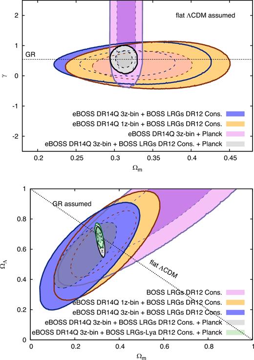
Top panel: Constraints on the gravity model through the dependence between Ωm and the γ index, when a flat ΛCDM model is assumed. The black horizontal dashed line displays the prediction for GR. All results are consistent with ΛCDM-Planck cosmology + GR. Bottom panel: Constraints on the flatness of the Universe and through the relation between Ωm and |$\Omega _\Lambda$| when GR is assumed as the theory of gravity. The black dashed line indicates the prediction for a flat Universe, |$\Omega _m+\Omega _\Lambda =1$|. The colour contours display different probe combination among eBOSS DR14Q (this work), the BOSS DR12 LRGs (Alam et al. 2017), BOSS DR12 Ly-α (du Mas des Bourboux et al. 2017; Bautista et al. 2017b), and CMB data from Planck Collaboration et al. 2016. All results are consistent with a flat-ΛCDM Universe.
The constraints derived by combining LRG BOSS results with DR14Q provide a measurement of γ with |$60\hbox{ per cent}$| precision and Ωm with |${\sim }10\hbox{ per cent}$|. These constraints become slightly better when we consider the DR14Q in three redshift bins (dark-blue contours), than in a single redshift bin (orange contours). The two top rows of Table 13 display the results for these two cases. Combining the DR14Q results with Planck measurements (magenta contours) does not provide a competitive constraint on γ due to the large errors of the fσ8 measurements. Certainly, γ regulates the amplitude of the fσ8 parameter as a function of redshift, and it is particularly sensitive to γ at low redshifts (see e.g. fig. 12 from Gil-Marín et al. 2016), where the BOSS LRG DR12 measurements dominate. Finally, we add all these three probes (grey contours) to obtain a |$35\hbox{ per cent}$| measurement on γ, as shown in the two bottom rows of Table 13, γ = 0.55 ± 0.19. All the studied probe combinations are consistent with GR predictions.
Measurements on Ωm and γ produced by combining various data sets, when a flat-ΛCDM Universe has been assumed. These measurements are indicated by the corresponding colour contours of Fig. 18. Using the eBOSS DR14Q at a single or at three overlapping redshift bins does not significantly affect the results, although the three redshift bin measurements have a slight larger constraining power on γ if Planck results are not used. In all the cases, the agreement of the measured cosmological parameters is in excellent agreement with GR predictions.
| Data set / Model | Ωm | γ |
|---|---|---|
| eBOSS DR14Q 3z-bin + BOSS LRGs DR12 Cons. + flat ΛCDM | |$0.313^{+0.040}_{-0.043}$| | 0.41 ± 0.28 |
| eBOSS DR14Q 1z-bin + BOSS LRGs DR12 Cons. + flat ΛCDM | |$0.332^{+0.041}_{-0.045}$| | 0.34 ± 0.31 |
| eBOSS DR14Q 3z-bin + BOSS LRGs DR12 Cons. + Planck + flat ΛCDM | |$0.3123^{+0.0072}_{-0.0074}$| | 0.55 ± 0.19 |
| eBOSS DR14Q 1z-bin + BOSS LRGs DR12 Cons. + Planck + flat ΛCDM | |$0.3127^{+0.0075}_{-0.0071}$| | 0.54 ± 0.19 |
In the bottom panel of Fig. 18, we relax the flatness condition and fix γ to be the predicted value by GR. We show the constraints on Ωm and |$\Omega _\Lambda$| when only the BOSS LRGs DR12 results are used (magenta contours). In this case, |$\Omega _\Lambda$| and Ωm present a large degeneracy that extends towards higher values of the Ω. Adding eBOSS DR14Q data, in orange contours when only a single redshift bin is used, and in blue contours when the three redshift bins are considered, considerably breaks this degeneracy. The resulting constraints are |$\lbrace \Omega _m, \, \Omega _\Lambda \rbrace =\lbrace 0.322^{+0.095}_{-0.101}, \, 0.64^{+0.15}_{-0.14} \, \rbrace$| for BOSS LRGs DR12 + eBOSS DR14Q using a single redshift bin, and |$\lbrace \Omega _m, \, \Omega _\Lambda \rbrace =\lbrace 0.239^{+0.091}_{-0.098}, \,0.57^{+0.15}_{-0.14} \, \rbrace$| when three redshift bins are used. Both results are similar and are in good agreement with a flat-ΛCDM Universe with Planck best-fitting parameters. In both cases, a Universe without Dark Energy (|$\Omega _\Lambda =0$|) is disfavoured by 4σ when only the BOSS LRGs DR12 and eBOSS DR14Q data sets are included. Adding the Planck and BOSS DR12 Ly α results to these two data sets provides tighter constraints on the density of matter, |$\Omega _m=0.3094^{+0.0076}_{-0.0080}$| (|$2.5\hbox{ per cent}$| precision), and on the density of Dark Energy |$\Omega _\Lambda =0.697^{+0.035}_{-0.032}$| (|$0.5\hbox{ per cent}$| precision), again in full agreement with a Universe with no curvature, Ωk = −0.007 ± 0.030.
8 CONSENSUS RESULTS
The RSD analysis in this paper is based on the eBOSS DR14 quasar sample in the redshift range 0.8 ≤ z ≤ 2.2, using the power-spectrum monopole, quadrupole, and hexadecapole measurements on the k-range, 0.02 ≤ k [h Mpc−1] ≤ 0.30, shifting the centres of k-bins by fractions of 1/4 of the bin size and averaging the four derived likelihoods. Applying the TNS model along with the 2-loop resumed perturbation theory, we are able to effectively constrain the cosmological parameters fσ8(z), H(z)rs(zd), and DA(z)/rs(zd) at the effective redshift zeff = 1.52, along with the remaining ‘nuisance’ parameters, b1σ8(z), b2σ8(z), Anoise(z) and σP(z), in all cases with wide flat priors.
This work is released along with four other complementary RSD analyses based on the exact same sample, including identical weighting schemes (described in Section 2.2), but using slightly different techniques and observables. The fiducial cosmology in which the sample has been analysed is also the same across papers. We briefly describe the other DR14Q works below.
Hou et al. (2018) perform a RSD analysis using Legendre polynomial with order ℓ = 0, 2, 4, and clustering wedges. They use ‘gRPT’ to model the non-linear matter clustering. For the RSD, they use a streaming model extended to one-loop contribution developed by Scoccimarro (2004) and Taruya et al. (2010) and a non-linear corrected FoG term. Finally, the bias modelling adopted is the one described in Chan & Scoccimarro (2012), which includes both local and non-local contributions. A modelling for spectroscopic redshift error is also included.
Ruggeri et al. (2018) present an RSD analysis using an optimized redshift-dependent weighting scheme presented in Ruggeri et al. (2017a,b). A Fourier space analysis is then applied, using evolving power-spectrum multipoles to measure cosmological parameters alongside with its evolution across the redshift bin.
Zarrouk et al. (2018) describe an RSD analysis using Legendre multipoles with ℓ = 0, 2, 4 and three wedges of the correlation function on the s-range from 16 h−1 Mpc to 138 h−1 Mpc. They use the Convolution Lagrangian Perturbation Theory with a Gaussian Streaming model and demonstrate its applicability for dark matter haloes of masses of the order of 1012.5 M⊙ hosting eBOSS quasar tracers at mean redshift z ≃ 1.5 using the or simulation.
The combined BAO and RSD analysis presented in Zhao et al. (2018) takes only into account the power-spectrum monopole and the quadrupole in the k-range of 0.02 ≤ k [h Mpc−1] ≤ 0.30. The power-spectrum template utilized is based on the regularized perturbation theory up to second order. With the optimal redshift weights, they constrain DA, H, and fσ8 at four effective redshifts 0.98, 1.23, 1.53, and 1.94.
All these papers provide constraints on the same cosmological parameters, fσ8(zeff) DA(z)/rd, H(z)rd (at least) at the effective redshift zeff = 1.52, and therefore their constrain can be easily compared.
Fig. 19 displays the constraints represented as contours for those companion paper RSD analyses described above, which do not apply any redshift weighting scheme: Hou et al. (2018) and Zarrouk et al. (2018) (both using the three configuration space multipoles analyses) along with this work. We focus on the variables with higher interest, fσ8, DA/rs and Hrs along with the linear bias, b1σ8, all evaluated at zeff = 1.52. The different analyses yield consistent results for the different measurements for the cosmological parameters using the methodologies described above. The obtained precision (which does not include the systematic error budget) is also comparable among the methods, with no significant difference among configuration space, and Fourier space methodologies.
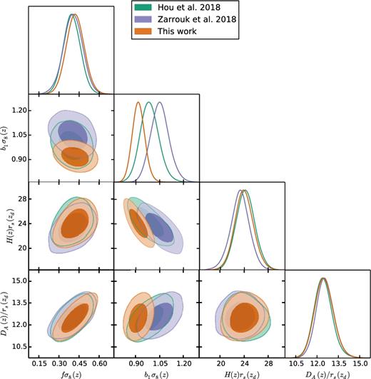
Parameter contours for b1σ8(zeff), fσ8(zeff), DA(zeff)/rs(zd), and H(zeff)rs(zd) for the predictions by the companion papers using the same DR14Q data set. Purple contours represent the prediction by Zarrouk et al. (2018) analysis and green contours the predictions by Hou et al. (2018); both analyses use the configuration space multipoles (see the text for details). Orange contours display the results presented in this work (using a single redshift bin). All the three analyses produce consistent values of cosmological parameters, fσ8, DA/rs, and Hrs, both in the actual measurement as well as in the size and shape of the confidence level contours. The ∼1σ difference on b1σ8 is caused by different prior conditions on the bias parameters and by the different bias models used (see the text for a further description).
The b1σ8 panels show a ∼1σ discrepancy between the Fourier space- and configuration space-based analyses. Further investigation has demonstrated that this behaviour is related to the different bias model assumptions used for the different papers. The configuration space model, as the one used by Zarrouk et al. (2018), depends on two bias parameters, F΄ and F΄, which are eventually related to b1 and b2. However, the two-point correlation function displays a limited sensitivity on F΄ so that this parameter is poorly constrained when fitting either Legendre multipoles with order ℓ = 0, 2, 4 or three wedges. Zarrouk et al. (2018) used mocks and N-body simulations to show that fixing the F΄ parameter to the peak-background split prediction improves the convergence of the fits without significantly shifting the cosmological parameters DA, H and fσ8. This prior on F΄ does, however, have an effect on F΄, and therefore on the derived b1σ8. Tests on the or mocks revealed a reduction on b1σ8 best-fitting value by a factor 0.037 when the described prior on F΄ is applied. Therefore, we conclude that the discrepancy among models in terms of b1σ8, at least for the configuration space model used by Zarrouk et al. (2018), can be understood by difference in bias prescriptions and does not affect the cosmological parameters studied in this set of papers.
For complementary comparisons among the wedges approach, as well as the comparison among weighting versus non-weighting schemes, we refer the reader to Zarrouk et al. (2018).
Two BAO additional analyses on the same DR14Q sample are released along with this paper: Wang et al. (2018) and Zhu et al. (2018), which are complementary to the isotropic analysis recently presented by Ata et al. (2018). These two analyses utilize the redshift weights proposed in Zhu et al. (2015) to compress the BAO information in the redshift direction on to a set of weighted correlation functions. These estimators provide optimized angular diameter distance and Hubble parameter measurements at all redshifts within the range of the quasar sample. Thus, this approach complements the traditional BAO analysis presented in Ata et al. (2018) by providing a first BAO measurement of the Hubble parameter from this sample.
8.1 Consensus between RSDand isotropic BAO
We compare the αiso values derived from the BAO analysis on the power-spectrum monopole with those derived from the RSD full-AP analysis on the power-spectrum monopole, quadrupole, and hexadecapole.
Combining the values of α∥ and α⊥ from the RSD analysis presented in Table 9, according to equation (18) produces, |$\alpha ^{\rm RSD}_{\rm iso}=1.003\pm 0.035$|, which corresponds to, |$D^{\rm RSD}_V(1.52)/r_s(z_d)=26.27\pm 0.93$|.
Similarly to the analysis in Ata et al. (2018), we perform a BAO analysis on the power-spectrum monopole. Unlike the approach of Ata et al. (2018), we apply the weighting scheme described in Section 2.2. The sole difference with the previous BAO analysis is our use of focal plane weights instead of the nearest neighbour weights used in Ata et al. (2018). However, neither of these weighting schemes has demonstrated any dependency on αiso (see Table 4), and therefore both approaches are expected to provide unbiased measurements. Performing the BAO fit in the range of scales 0.02 ≤ k [h Mpc−1] ≤ 0.30 yields |$\alpha ^{\rm BAO}_{\rm iso}=1.003\pm 0.043$|, 15 which corresponds to |$D^{\rm BAO}_V(1.52)/r_s(z_d)=26.27\pm 1.11$|. We do not provide more details on the BAO fit in this paper, as the results are similar to those presented in Ata et al. (2018).
Both results are in excellent agreement, although, given the identical data set, we expect a high correlation between them.
The left-hand panel of Fig. 20 displays the inferred αiso parameter: from a BAO analysis using P(0) in the x-axis and from the RSD analysis using the three described power-spectrum multipoles in the y-axis. The symbols display the results for the 1000 ez mock realizations and the data using the different redshift estimates, represented by the coloured symbols following the same colour-notation than in Fig. 8. The right-hand panel displays the comparison between the 1σ error using the same plot-notation. As expected, the correlation between the two techniques is visibly large, and there is a correlation between the inferred errors in the right-hand panel. The results from the mocks show that the RSD analyses using the mentioned three power-spectrum multipoles tend to present a smaller error on αiso with respect to the BAO analysis on the monopole. For both cases, the quantities computed from the data are in good agreement with those observed from the mocks.
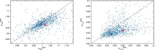
Comparison between the isotropic BAO scale parameter αiso (left-hand panel) and its error |$\sigma _{\alpha _{\rm iso}}$| (right-hand panel), inferred from a BAO fit on the power-spectrum monopole, and from an RSD analysis using the power-spectrum monopole, quadrupole, and hexadecapole. In the first case, αiso is inferred from the BAO peak position in the monopole, whereas in the former case αiso is inferred from α∥ and α⊥ through equation (18). The blue dots represent the measurement for the 1000 ez mocks, whereas the coloured crosses represent the data when zfid (orange cross), |$z_{\rm Mg\, {\small II}}$| (red cross), and zPCA (black cross) are used as redshift estimates. The observed correlation between these mocks with 0.9 ≤ αiso ≤ 1.1 in both RSD and BAO measurements is ρ = 0.66. The results obtained from the three data sets represent a typical realization with respect to the mocks.
9 CONCLUSIONS
In this paper, we perform an RSD analysis on the 2-yr data of SDSS-IV eBOSS quasar sample (DR14), which consists of 148 659 quasars at 0.8 ≤ z ≤ 2.2 and measures the cosmological parameters: the logarithmic growth of structure times the amplitude of the dark matter fluctuations, fσ8, the angular diameter distance of the sound horizon scale at drag redshift, DA/rs, and the Hubble parameter times the sound horizon scale at drag redshift, Hrs, all at the effective redshift of zeff = 1.52. We combine the measurements on the power-spectrum monopole, quadrupole, and hexadecapole on the scale range 0.02 ≤ k [h Mpc−1] ≤ 0.30, with a theoretical model based on two-loop resumed perturbation theory and TNS model for redshift space distortions and measure fσ8(zeff) = 0.420 ± 0.076, |$H(z_{\rm eff})=[162\pm 12]\, (r_s^{\rm fid}/r_s)\,{\rm km s}^{-1}\,{\rm Mpc}^{-1}$| and |$D_A(z_{\rm eff})=[1.85\pm 0.11]\times 10^3\,(r_s/r_s^{\rm fid}){\rm Mpc}$|. These results include a systematic error budget that contains contributions from both observational and modelling systematics, extracted from realistic N-body mocks. Additionally, we perform a large number of systematic tests and demonstrate that the cosmological results are robust and unbiased by the choice of parametrization, e.g. the k-sampling of the data, the covariance matrix model, the redshift estimate used in the data, or the range of scales used in the fit.
Additionally, we divide the full redshift range into three overlapping redshift ranges, 0.8 ≤ z ≤ 1.5, 1.2 ≤ z ≤ 1.8, 1.5 ≤ z ≤ 2.2, and measure the same quantities in each individual bin. Since the redshift bins overlap we also compute the covariance among the different parameters at different bins using a set of 1000 mocks. These results are presented along with their covariance matrix in Table 12. We have found that for the intermediate redshift bin the best-fitting χ2 value is higher than any result found in the mocks. After removing the frequency k ≃ 0.11 h Mpc on the monopole and quadrupole the χ2 value is reduced to typical values. We have checked that this does not have a significant impact on the derived cosmological parameters. We leave for a future work the study and characterization of this systematic effect. Finally, we combine the derived cosmological parameters with other complementary data sets, such as the cosmological measurements from the SDSS-III DR12 LRG BOSS sample and CMB measurements from Planck. When we perform a null-test of gravity, γ = 0.54 ± 0.19 for a flat-ΛCDM Universe, which is fully consistent with the GR predictions. Using the same data sets, we relax the ‘flatness’ condition and measure |$\Omega _\Lambda =0.697^{+0.035}_{-0.032}$| and |$\Omega _m=0.3094^{+0.0076}_{-0.0080}$| assuming GR as the theory of gravity. Both measured Ω values are fully consistent with a flat-ΛCDM Universe, Ωk = −0.007 ± 0.030.
We have performed a comparison with the companion papers (Hou et al. 2018 and Zarrouk et al. 2018) that offers complementary analysis on the same data sample and find an excellent agreement both in the parameters measured as well on the errors and correlation among cosmological parameters.
We now compare our results with those forecasted at the beginning of the survey in Zhao et al. (2016). Table 14 displays, in the first column, the forecasted errors for a final area of 7500 deg2 in the redshift range 0.6 ≤ z ≤ 2.2 for the cosmological parameters of interest. The second column lists the scaling of those constraints to the volume of the current DR14Q sample. The scaling factor is 2.07, computed as the square-root of the ratio of volumes, assuming a constant density of quasars across the redshift range. The third column presents the errors in this work for the zfid redshift estimate when the power-spectrum monopole, quadrupole, and hexadecapole are used. There is an excellent agreement between the errors of the scaled forecasted AP parameters DA, H, and DV and those obtained in this work. The scaled forecasted errors for fσ8 and b1σ8, however, present a 3.5 factor of disagreement with those measured. The reason for this is that the forecasts on fσ8 and b1σ8 presented by Zhao et al. (2016) are performed without marginalising over DA or H. When this marginalization is taken into account, we obtain re-scaled errors for fσ8 and b1σ8 of 0.140 and 0.032, respectively. These results are just |${\sim }20\hbox{ per cent}$| larger than those we report in this paper. Such small differences could originate from the idealized theoretical model used in the Fisher forecast or by large statistical fluctuations on the uncertainties (as found in the mocks). We conclude that the current analysis on the first 2 yr of data from eBOSS quasar sample is in full agreement with the initial forecasts, and, consequently, the forecasted precision by the end of survey will be likely achieved in the final data release of quasars in 2019–2020.
Comparison between the statistical-only errors obtained in this paper, labelled as ‘This work’, and those forecasted at the beginning of the survey (see table 4 of Zhao et al. 2016), labelled as ‘Forecast’. The column ‘Re-scaled Forecast’ represents the ‘Forecast’ column scaled by the square-root of the ratio of volumes between the one assumed by Zhao et al. (2016) at the end of the eBOSS survey, and one corresponding to this survey. The scaling factor corresponds to 2.07 (see the main text). The agreement found is very high in the AP-scale parameters DA, H and DV. On the other hand, the fσ8 and b1σ8 error forecast were performed without marginalizing with respect DA and H, and consequently, their errors are smaller. When this marginalization is taken into account, we find |$\sigma _{f\sigma _8}/f\sigma _8=0.14$| and |$\sigma _{b_1\sigma _8}/b_1\sigma _8=0.032$|, which are in agreement with the findings of this work.
| Forecast | Re-scaled forecast | This work | |
|---|---|---|---|
| |$\sigma _{D_A}/D_A$| | 0.025 | 0.052 | 0.051 |
| σH/H | 0.033 | 0.069 | 0.063 |
| |$\sigma _{D_V}/D_V$| | 0.016 | 0.033 | 0.035 |
| |$\sigma _{f\sigma _8}/f\sigma _8$| | 0.028 | 0.058 | 0.16 |
| |$\sigma _{b_1\sigma _8}/b_1\sigma _8$| | 0.006 | 0.012 | 0.042 |
This work, alongside the above quoted companion papers, for the first time measures the cosmological parameters fσ8, DA, and H, using the full-shape analysis of power-spectrum multipoles of eBOSS DR14 quasars as dark matter tracers, demonstrating the feasibility of this new dark matter tracer not only for Ly α-based analyses but also in terms of galaxy clustering to infer cosmological parameters. Previous works have begun to explore the >0.8 redshift range using emission line galaxies (ELGs) (FastSound16; Okumura et al. 2016) and from a multisample of galaxies (VIPERS), Mohammad et al. 2018), and performed fσ8 measurements using the full shape of the monopole and quadrupole. This paper, along with the companion papers, improve in terms of precision, but also extends the inferred cosmological parameters from a single fσ8 measurement without marginalization to a multipole {fσ8, DA/rs, Hrs} set of marginalized parameters. For instance, Okumura et al. (2016) and Mohammad et al. (2018) measure fσ8 with |${\sim }25\hbox{ per cent}$| precision at a fixed DA and H, whereas in this paper we find fσ8 with |$18\hbox{ per cent}$| precision, fully marginalizing over DA and H, and |${\sim } 10\hbox{ per cent}$| when setting H × DA to a fiducial value. We expect these errors to be reduced by a factor of ∼2 by the completion of the eBOSS survey. The quasars sample as dark matter tracer represents only one aspect of the eBOSS programme. Separate RSD and BAO analyses of the eBOSS LRGs and ELGs samples will fill in the z ∼ 0.8 region with more cosmological measurements in the next year (see Bautista et al. 2017a for the first BAO measurement using the DR14 LRG sample), helping to complete the cosmological distance ladder measurements from z ∼ 0 to z ∼ 3 presented in Fig. 17.
Future galaxy spectroscopic surveys such as the ground-based Dark Energy Spectroscopic Instrument (DESI;17 DESI Collaboration et al. 2016a,b) and the space missions such as EUCLID18 (Amendola et al. 2013) will after the year 2020 extensively probe the intermediate redshift range 1 ≤ z ≤ 2, providing cosmological measurements with unprecedented precision. The eBOSS-related papers represent the first step in obtaining measurements at this previously unexplored region.
ACKNOWLEDGEMENTS
This work has been done within the Labex ILP (reference ANR-10-LABX-63) part of the Idex SUPER and received financial state aid managed by the Agence Nationale de la Recherche as part of the programme Investissements d'avenir under the reference ANR-11-IDEX-0004-02.
G.B.Z. is supported by NSFC Grants 1171001024 and 11673025. G.B.Z. is also supported by a Royal Society Newton Advanced Fellowship, hosted by University of Portsmouth.
S.H. and K.H. work was supported under the U.S. Department of Energy contract DE-AC02-06CH11357.
G.R. acknowledges support from the National Research Foundation of Korea (NRF) through Grant No. 2017077508 funded by the Korean Ministry of Education, Science and Technology (MoEST), and from the faculty research fund of Sejong University in 2018.
Funding for SDSS-III and SDSS-IV has been provided by the Alfred P. Sloan Foundation and Participating Institutions. Additional funding for SDSS-III comes from the National Science Foundation and the U.S. Department of Energy Office of Science. Further information about both projects is available at www.sdss.org. SDSS is managed by the Astrophysical Research Consortium for the Participating Institutions in both collaborations. In SDSS-III these include the University of Arizona, the Brazilian Participation Group, Brookhaven National Laboratory, Carnegie Mellon University, University of Florida, the French Participation Group, the German Participation Group, Harvard University, the Instituto de Astrofisica de Canarias, the Michigan State/Notre Dame/JINA Participation Group, Johns Hopkins University, Lawrence Berkeley National Laboratory, Max Planck Institute for Astrophysics, Max Planck Institute for Extraterrestrial Physics, New Mexico State University, New York University, Ohio State University, Pennsylvania State University, University of Portsmouth, Princeton University, the Spanish Participation Group, University of Tokyo, University of Utah, Vanderbilt University, University of Virginia, University of Washington, and Yale University.
The Participating Institutions in SDSS-IV are Carnegie Mellon University, Colorado University, Boulder, Harvard-Smithsonian Center for Astrophysics Participation Group, Johns Hopkins University, Kavli Institute for the Physics and Mathematics of the Universe Max-Planck-Institut fuer Astrophysik (MPA, Garching), Max-Planck-Institut fuer Extraterrestrische Physik (MPE), Max-Planck-Institut fuer Astronomie (MPIA Heidelberg), National Astronomical Observatories of China, Observatorio Naciona/MCTI, New Mexico State University, New York University, The Ohio State University, Penn State University, Shanghai Astronomical Observatory, United Kingdom Participation Group, University of Portsmouth, University of Utah, University of Wisconsin, and Yale University.
This work made use of the facilities and staff of the UK Sciama High Performance Computing cluster supported by the ICG, SEPNet, and the University of Portsmouth. This research used resources of the National Energy Research Scientific Computing Centre (NERSC), a DOE Office of Science User Facility supported by the Office of Science of the U.S. Department of Energy under Contract No. DE-AC02-05CH11231.
This research used resources of the Argonne Leadership Computing Facility, which is a DOE Office of Science User Facility supported under contract DE-AC02-06CH11357.
Footnotes
The WiggleZ Dark Energy Survey, wigglez.swin.edu.au/.
The VIMOS Public Extragalactic Redshift Survey (VIPERS), http://vipers.inaf.it/.
We follow the effective volume definition by equation (5) of Tegmark (1997).
Sector is defined as the union of spherical polygons defined by a unique intersection of spectroscopic tiles. See table 1 of Reid et al. (2016) for further details and definitions.
Here, we define the effective redshift as the sum of the redshifts of an object, |$z({\boldsymbol r}_i)$|, weighted by the total weight of equation (5), divided by the weighted number of objects, |$z_{\rm eff}\equiv \sum _i z({\boldsymbol r}_i)w_{\rm tot}({\boldsymbol r}_i)/\sum _i w_{\rm tot}({\boldsymbol r}_i)$|.
Fastest Fourier Transform in the West: http://fftw.org
This is the approach followed in Beutler et al. 2014 (see equation 40).
The degrees of freedom are just 28-6 and 28-4, respectively, because Anoise does not contribute to the shape of the quadrupole or hexadecapole, nor do the bias parameters (b1, b2) contribute to the shape of the hexadecapole.
Note that the clustering of ez and qpm mocks reported in the fig. 6 of Ata et al. (2018) is slightly different from the one reported here, specially at small scales. Such differences are caused by the effect of redshift failure and fibre collisions, which were not included in the mocks used in Ata et al. (2018).
We combine the results of the four different k-bin centres by averaging their normalized likelihood for each individual parameter.
We account for those realizations with double detection of αiso for both ez- and qpm-derived covariances, in total 962 out of 1000 mocks.
σ+ and σ− are defined in such a way that xbf ± σ± corresponds to |$\chi _{\rm min}^2+1$|.
BAO or RSD analyses are not able to measure DA(z) or H(z) independently from the sound horizon scale at the baryon drag epoch, rs(zd), which is usually taken from CMB measurements. However, this scale can be computed from models of Big Bang Nucleosynthesis, and therefore, one can consider RSD and BAO derived quantities independent from the CMB data
In this paper, we always use Planck cosmology to refer to those results on H0, Ωm, and σ8 derived from the TT+TE+EE+lowP, fifth column from table 3 of Planck Collaboration et al. (2016).
This measurement slightly differs from the value found in Ata et al. (2018) when the power spectrum alone was used in the scale range 0.02 ≤ k [h Mpc−1] ≤ 0.23, αiso = 0.992 ± 0.040 (see ‘P(k) (combined)’ in table 5 of the quoted paper). However, this small difference on αiso is not significant, given the slight differences in terms of the analysis described in the main text.
The Subaru FMOS galaxy redshift survey, http://www.kusastro.kyoto-u.ac.jp/Fastsound/
DESI, http://desi.lbl.gov/
REFERENCES
APPENDIX A: Isotropic-α approximation
In this appendix, we examine the assumption of |$\alpha _{\rm iso}=\alpha _\parallel ^{1/3}\alpha _\perp ^{2/3}$| used in some sections of the paper. Ross et al. (2015) derive the analytic formulae for the parameter combination among α∥ and α⊥ inferred from the different power spectrum and correlation function μ-moments given by Legendre polynomials, showing explicitly what is being measured by each. Briefly, when the variable |$\alpha _F^{m+n}=\alpha _\parallel ^m\alpha _\perp ^n$| is defined, the m and n values that provide the degenerate directions of these parameters, given the observed multipole at linear order, are reported. For the power-spectrum monopole, m = 1/A(1/3 + 2β/5 + β2/7) and n = 1/A(2/3 + 4/15β + 2/35β2), where β ≡ b1/f and A ≡ 1 + 2/3β + 1/5β2. For the b1 and f values obtained from the mean of the ez mocks, b1 = 2.25 and f = 0.924, β = 0.4107. Thus, the measurement of the power-spectrum monopole in redshift space provides a degenerate direction corresponding to |$\alpha _F=\alpha _\parallel ^m\alpha _\perp ^n$| with m = 0.399 and n = 0.601, which differs slightly from the expected values when the redshift space distortions are removed (in the reconstruction process for example) m = 0.333 and n = 0.667. The measurement of the μ2-moment of the power spectrum (in some sense equivalent to the quadrupole) provides m = 0.336 and n = 0.1856. The top panel of Fig. A1 shows the degenerate direction for these two cases described above, |$1=\alpha _\parallel ^m \alpha _\perp ^n$|, along with the α∥ and α⊥ measurement from the individual ez mocks. Visually, the μ-square moment case is disfavoured with respect to the monopole cases (with or without RSD), suggesting that when both monopole and quadrupole are added, the total signal remains dominated by the monopole, as the signal-to-noise ratio is higher. The lower panel presents the histogram of the quantity |$\alpha _\parallel ^m\alpha _\perp ^n-{\alpha |_{\epsilon =0}}^{m+n}$| computed from the same mocks, where we denote α|ε = 0 as the value of α computed when α∥ and α⊥ are set to the same value. The histogram displays the degree of distortion compared to the isotropic case (both α being equal) with the full-AP test. Again, the case for m = 0.399 and n = 0.601 (P(0) no-RSD) presents a distribution with lower dispersion than the one by m = 0.336 and n = 0.1856 (P(2) RSD). We conclude that the quantity DV is well constrained when α∥ = α⊥.
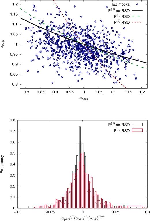
Top panel:ez mock measurements for α∥ and α⊥ for the full-AP test (blue symbols) along with the degeneracy directions predicted by Ross et al. (2015) when only the monopole is used after (black solid line) and before (green dashed line) the RSD are removed, and when the μ2-moment is used (red dotted line). The mocks display a degenerate direction on |$\alpha =\alpha _{\parallel }^m\alpha _\perp ^{n}$| that is close to the one predicted by monopole with RSD removal, which corresponds to αiso. Bottom panel: Histogram of the quantity |$\alpha _\parallel ^m\alpha _\perp ^n-{\alpha |_{\epsilon =0}}^{m+n}$| computed from the mocks above, where α|ε = 0 is the α parameter obtained when we set α∥ to be equal to α⊥. The black bands display the results for m and n when m = 1/3 and n = 2/3, corresponding to the black solid line in the top panel figure, and the red bands for m = 0.336 and n = 0.1856, corresponding to the red dotted line in the top panel.
APPENDIX B: SURVEY GEOMETRY
APPENDIX C: EFFECT OF SPECTROSCOPIC WEIGHTS IN THE POWER-SPECTRUM MULTIPOLES
Table 4 lists the results of our test of the impact of the weights wfoc and wcp on the cosmological parameters of interest. In this appendix, we describe the effect of such weights in the clustering amplitude and shape of the power-spectrum monopole, quadrupole, and hexadecapole. In order to measure the potential deviations caused by the spectroscopic weights, we compute the power-spectrum multipoles on the ez mocks before such effects are applied (‘raw’ measurements of Table 4) and take the mean value over the 1000 realizations. We adopt this measurement as a clustering reference. We apply the different weighting schemes on individual mocks and compare their mean with the reference mean. The results are shown in Fig. C1, where the reference measurement is presented as dashed black lines in the top sub-panels. zf represents the correction of the redshift failures through the wfoc weights according to equation (2). wfocwcp corresponds to the case where both fibre collisions and redshift failures are applied following the prescription described in Section 2.2.1. Finally, wnozwcp corresponds to the case where both fibre collisions and redshift failures are included, but in this case, the redshift failures have been corrected using the near-neighbour technique. The top sub-panels present the actual power-spectrum multipole measurement, kP(ℓ), and the bottom sub-panels the difference with respect to the reference case, |$k\Delta P^{(\ell )}\equiv kP^{(\ell )}_i-kP^{(\ell )}_{\rm raw}$|. In the top sub-panels, the error-bar is not indicated, as it would be too small to be distinguished from the actual lines. In the bottom sub-panels, the black dotted lines represent the expected 1σ statistical error for the data DR14Q sample, and has been computed as the rms of the 1000 realizations of the mocks (those with the wfocwcp weighting scheme).
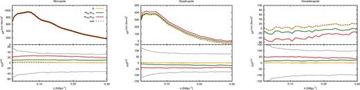
Effect of the different spectroscopic weights in the power-spectrum monopole (left-hand panel), quadrupole (middle panel), and hexadecapole (right-hand panel) on the mean of 1000 realizations of the ez mocks. The top sub-panels display the quantity kP(ℓ) for the different weighting schemes (see the text and Table 4 for reference) in different cases. The bottom sub-panels display the difference with respect to the ‘raw’ case, where no observational effect has been applied. The black dotted lines correspond to the expected 1σ statistical error corresponding to the DR14Q sample and computed from the rms of the 1000 realizations.
zf tests the isolated effect of the focal plane weights (without the fibre collisions) through wfoc. Both Table 4 and Fig. C1 demonstrate that wfoc perfectly accounts for the redshift failures, being able to recover the original power spectrum signal for the three studied multipoles. Conversely, when the nearest neighbour technique is applied (both for correcting the fibre collision and the redshift failures), a spurious anisotropic signal is introduced in such a way that the monopole and hexadecapole are underestimated, whereas the quadrupole is overestimated. This anisotropic signal contaminates and biases the measurement of fσ8, as discussed in Section 5.2. In this case, we observe that the spurious signal is higher when the nearest neighbour technique is applied to correct the redshift failure weights. The systematics associated with the inaccuracy when correcting the fibre collision effect through the nearest neighbour technique are discussed in Section 5.2.
APPENDIX D: FULL COVARIANCE MATRICES
In this section, we compare the covariance matrices for the power-spectrum multipoles, ℓ = 0, 2, 4 when they are estimated from 400 realizations of the qpm mocks and the 1000 realizations of the ez mocks. Fig. D1 displays the off-diagonal elements (cross-correlation coefficients) of the covariance, when the k-binning is linear between 0.01 h Mpc−1 up to 0.40 h Mpc−1. The left(right)-hand panel displays the terms computed from the qpm(ez) mocks. The scale for the correlation coefficients has been defined in the range of 0–0.16 in order to stress the off-diagonal signal. The diagonal elements are by definition 1 and lie out of the scale. In general, both matrices are dominated by their diagonal component, as the off-diagonal cross-correlation terms are typically small, <0.1. The different degree of noise from the qpm- and ez-derived covariances is caused by the different number of realizations from which the two covariances are computed.
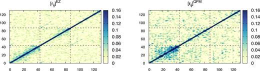
Cross-correlation terms, |$r_{ij}\equiv \sigma _{ij}/\sqrt{\sigma _{ii}^2\sigma ^2_{jj}}$|, corresponding to the covariance matrices inferred from 400 realizations of qpm mocks and 1000 realizations of ez mocks in the left-hand and right-hand panels, respectively. For each panel, from the left to the right, the monopole, quadrupole, and hexadecapole k-bin terms are represented and separated by the dashed black lines. For each of the multipoles, the covariance elements correspond to a linear k-binning between 0.01 ≤ k [h Mpc−1 ≤ 0.40. The colour scale has been adjusted to highlight the off-diagonal terms. The terms in the diagonal have by definition a cross-correlation term of 1 and lie out of the scale. The qpm-derived covariance present higher values of the off-diagonal terms, specially on the monopole, whereas the ez-derived covariance is more diagonal, but this effect is minor compared to the differences observed in the diagonal terms, as displayed by Fig. D2.
Fig. D2 displays the ratio of the diagonal elements of the two covariances for the three studied power-spectrum multipoles in different colours. Both covariances are in agreement, although the qpm-derived elements tend to be |${\sim }5\hbox{ per cent}$| larger than those of the ez-derived covariance for the monopole and quadrupole. However, this trend is not maintained on the hexadecapole, neither for the monopole at small k. The impact of the covariance choice in the parameter estimation of the data is discussed in Section 5.3.
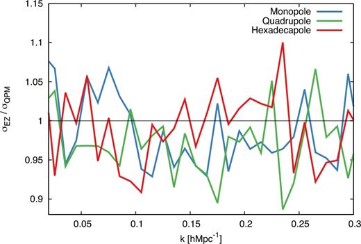
Ratio of the square root of the diagonal terms of the covariance matrices, σii, inferred from 400 realizations of qpm mocks and 1000 realizations of eq mocks, |$\sigma _{ii}^{\rm qpm} / \sigma _{ii}^{\rm ez}$|, for the monopole (in blue), quadrupole (in green), and hexadecapole (in red). As a general trend for the monopole and quadrupole, the qpm-derived errors tend to be five times larger than in the ez-derived errors.
APPENDIX E: GAUSSIAN APPROXIMATION OF THE LIKELIHOOD
In this appendix, we compare the full mcmc contours resulting from the actual data set with those resulting from the Gaussian approximation used in Sections 6.1–6.3 to compute the reported data vectors and covariance matrices. For all the cases, the data vector is taken as the mean of the considered mcmc steps. Fig. E1 displays the posterior-likelihood for the anisotropic fit when the full-redshift range 0.8 ≤ z ≤ 2.2 is considered (corresponding to Section 6.2). The contours drawn from the mcmc-full chain are represented in purple. On the other hand, the green and orange contours correspond to the Gaussian approximation when (i) all the mcmc step chains are used to compute the Gaussian covariance and central data vectors (orange contours); and (ii) only those steps contained within |$\chi ^2\le \chi ^2_{\rm min}+14.16$| are used to compute the Gaussian covariance (green contours). The former case is the one used to compute the data vector and covariance presented in equations (28) and (29) (without the diagonal systematic contribution). In this sense, Fig. E1 demonstrate the excellent agreement between the actual mcmc posterior likelihood surface and the reported Gaussian approximation. In this case, full mcmc distribution do not present strong non-Gaussian tails, and consequently, the Gaussian predictions from (i) and (ii) are very similar.
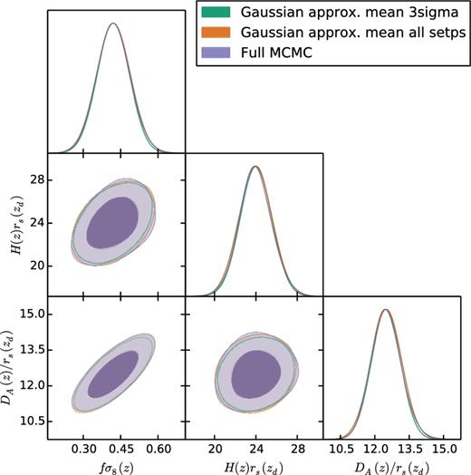
Posterior likelihood for the cosmological parameters of interest corresponding the DR14Q data set when the full redshift range, 0.8 ≤ z ≤ 2.2, is considered as a single redshift bin. The contours drawn from the full mcmc steps are represented in purple. In addition, a Gaussian approximation to the full mcmc steps is also plotted when (i) all the mcmc step chains are used to compute the Gaussian covariance and central data vectors values; and (ii) only those steps within |$\chi ^2\le \chi ^2_{\rm min}+14.16$| are used to compute the Gaussian covariance parameters and data vector values. The agreement between all three cases demonstrate the high degree of Gaussianity of the original sample drawn from the full mcmc steps.
On the other hand, Fig. E2 displays the posterior likelihood corresponding to Section 6.3, when the DR14Q data set is divided into three overlapping redshift bins: highz (right-hand panel), midz (middle panel), and lowz (left-hand panel). Green contours display the full mcmc steps when a very broad and flat prior is applied on α∥ and α⊥. We refer to this prior: 0 ≤ α⊥, ∥ ≤ 2 as ‘soft prior’. On the other hand, the purple contours result from applying the prior displayed by Table 11 and we refer them as ‘hard prior’. These priors are defined to cut-off the secondary minima outside the range 0.8 ≤ α∥, ⊥ ≤ 2.2. The ‘hard prior’ contours for the three redshift bins are overplotted in Fig. 15. Finally, the orange contours display the Gaussian approximation applying the (ii) approach described above on the mcmc steps with the ‘hard prior’ condition. These represent the covariance matrix given by Table 12. Unlike the single bin case presented in Fig. E1, the Gaussian approximation on the three overlapping redshift bins does not result in an excellent agreement. The reason is that when cutting off the data set in three chunks, the errors increases and non-Gaussian tails and secondary minima appear as a result of shifting the BAO features into the noisy spectrum of the data. We envision that by the end of eBOSS, the data collected by the survey will be sufficiently large that these secondary minima will disappear without the necessity of applying these hard prior conditions.
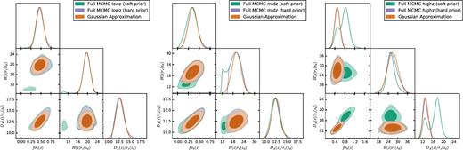
Posterior likelihood for the cosmological parameters of interest corresponding the DR14Q data set for the lowz, midz, and highz redshift bins in the left-hand, middle, and right-hand panels, respectively. Green contours display the results when a ‘soft’ flat prior is applied on the dilation scale factors: 0 ≤ α⊥, ∥ ≤ 2. In this case, secondary minima appear for some parameters, being the full distribution highly non-Gaussian. Purple contours display the results when a more restrictive ‘hard’ flat prior (given by Table 11) is applied. In this case, the secondary minima are cut-off and the mcmc steps describe a single-peaked distribution. Finally, the orange contour display the Gaussian approximation following the approach described by (ii) (see the text) applied to the mcmc steps with the ‘hard’ prior.
