


Abstract
Galaxy cluster Abell 3827 hosts the stellar remnants of four almost equally bright elliptical galaxies within a core of radius 10 kpc. Such corrugation of the stellar distribution is very rare, and suggests recent formation by several simultaneous mergers. We map the distribution of associated dark matter, using new Hubble Space Telescope imaging and Very Large Telescope/Multi-Unit Spectroscopic Explorer integral field spectroscopy of a gravitationally lensed system threaded through the cluster core. We find that each of the central galaxies retains a dark matter halo, but that (at least) one of these is spatially offset from its stars. The best-constrained offset is |$1.62^{+0.47}_{-0.49}$| kpc, where the 68 per cent confidence limit includes both statistical error and systematic biases in mass modelling. Such offsets are not seen in field galaxies, but are predicted during the long infall to a cluster, if dark matter self-interactions generate an extra drag force. With such a small physical separation, it is difficult to definitively rule out astrophysical effects operating exclusively in dense cluster core environments – but if interpreted solely as evidence for self-interacting dark matter, this offset implies a cross-section σDM/m ∼ (1.7 ± 0.7) × 10−4 cm2 g−1 × (tinfall/109 yr)−2, where tinfall is the infall duration.
INTRODUCTION
Many lines of evidence now agree that most mass in the Universe is in the form of dark matter, which interacts mainly via the force of gravity. The identity and detailed phenomenology of dark matter remain poorly understood. However, its gravitational attraction pulls low-mass systems into a series of hierarchical mergers through which dark and ordinary matter are gradually assembled into giant clusters of galaxies (Davis et al. 1985).
The typically smooth distribution of light in galaxy clusters visible today shows that merging systems have their gas content efficiently removed into the intracluster medium by ram pressure stripping, even while they pass the virial radius (Smith et al. 2010; Wu et al. 2013). The longevity of accompanying dark matter is less well understood, but the time-scale for its dissipation is a key ingredient in semi-analytic models of structure formation (Dariush et al. 2010). Full numerical simulations predict that the dark matter is eventually smoothed (Gao et al. 2004; Nagai & Kravtsov 2005; Bahé et al. 2012), but disagree about the time-scale and the radius/orbits on which stripping occurs (Diemand, Kuhlen & Madau 2007; Peñarrubia, McConnachie & Navarro 2008; Wetzel, Cohn & White 2009). Observations have shown that, as L* galaxies enter a galaxy cluster from the field, tidal gravitational stripping of their dark matter (Mandelbaum et al. 2006; Parker et al. 2007; Gillis et al. 2013) reduces their masses by ∼1013 M⊙ to ∼1012 M⊙ from a radius of 5 Mpc to 1 Mpc (Limousin et al. 2007, 2012; Natarajan et al. 2009). This stripping occurs at a rate consistent with simulations, but has not been followed to the central tens of kiloparsecs, which is where the predictions of simulations disagree.
Mergers of dark matter substructures into a massive galaxy cluster also reveal the fundamental properties of dark matter particles. The different non-gravitational forces acting on dark matter and standard model particles have been highlighted most visibly in collisions like the ‘Bullet Cluster’ 1E0657-56 (Clowe, Gonzalez & Markevitch 2004; Bradač et al. 2006; Clowe et al. 2006), Abell 520 (Mahdavi et al. 2007; Clowe et al. 2012; Jee et al. 2014), MACSJ0025-12 (Bradač et al. 2008), Abell 2744 (Merten et al. 2011) and DLSCL J0916.2+2951 (Dawson et al. 2012), and others (Harvey et al. 2015). Infalling gas (of standard model particles) is subject to ram pressure and tends to lag behind non-interacting dark matter (Young et al. 2011). Measurements of this lag yielded an upper limit on dark matter's self-interaction cross-section σ/m < 1.2 cm2 g−1 if the particle momentum exchange is isotropic, or σ/m < 0.7 cm2 g−1 if it is directional (Randall et al. 2008; Kahlhoefer et al. 2014). More interestingly still, if dark matter has (even a small) non-zero self-interaction cross-section, infalling dark matter will eventually lag behind old stars (Massey, Kitching & Nagai 2011; Williams & Saha 2011; Kahlhoefer et al. 2014; Harvey et al. 2013, 2014). Self-interactions confined within the dark sector can potentially have much larger cross-sections than those between dark matter and standard model particles, which are constrained by collider and direct detection experiments (e.g. Peter et al. 2013).
The galaxy cluster Abell 3827 (RA = |$22^{\rm h}01^{\rm m}49{^{\rm s}_{.}}1$|, Dec = −59° 57′ 15″, z = 0.099, X-ray luminosity LX = 8 × 1044 erg s−1 in the 0.1–2.4 keV band; De Plaa et al. 2007) is particularly interesting for substructure studies because it hosts the remnant stellar nuclei of four bright elliptical galaxies within the central 10 kpc. Such corrugation of the stellar distribution is very rare: only Abell 2261 (Coe et al. 2012; Postman et al. 2012) and MACSJ0717 (Jauzac et al. 2012; Limousin et al. 2012) are even comparably corrugated. All three clusters are still forming, through several simultaneous mergers – and can be used to investigate the late-stage dissipation of dark matter infalling through the same environment. Moreover, Abell 3827 has a unique strong gravitational lens system threaded between its multiple central galaxies (Carrasco et al. 2010). This enables the distribution of its otherwise invisible dark matter to be mapped (for reviews of gravitational lensing, see Bartelmann & Schneider 2001; Refregier 2003; Hoekstra & Jain 2008; Bartelmann 2010; Massey, Kitching & Richard 2010a; Kneib & Natarajan 2011). The cluster even lies within the optimum redshift range 0.05 < z < 0.1 to measure small physical separations between dark and ordinary matter (Massey et al. 2011).
Indeed, ground-based imaging (Williams & Saha 2011; Mohammed et al. 2014) suggests that dark matter associated with one of the central galaxies in Abell 3827 (the one where its position is best constrained, ‘nucleus’ N.1) is offset by ∼3 arcsec (6 kpc) from the stars. Such offsets are not seen in isolated field galaxies (e.g. Koopmans et al. 2006; Gavazzi et al. 2007). Interpreting the offset via a model in which tinfall is the time since infall, implies a lower limit of σ/m > 4.5 × 10⁻⁶(tinfall/1010 yr)−2 cm2 g−1. This is potentially the first detection of non-gravitational forces acting on dark matter.
In this paper, we present new Hubble Space Telescope (HST) imaging and Very Large Telescope (VLT) integral-field spectroscopy to hone measurements of the dark matter distribution. We describe the new data in Section 2, and our mapping of visible light/dark matter in Section 3. We describe our results in Section 4, and discuss their implications in Section 5. We conclude in Section 6. Throughout this paper, we quote magnitudes in the AB system and adopt a cosmological model with ΩM = 0.3, |$\Omega _\Lambda = 0.7$| and H0 = 70 km s−1 Mpc−1, in which 1 arcsec corresponds to 1.828 kpc at the redshift of the cluster.
DATA
HST imaging
We imaged the galaxy cluster Abell 3827 using the HST, programme GO-12817. Observations with the Advanced Camera for Surveys (ACS)/Wide Field Channel (WFC) during 2013 October consisted of 5244 s in optical band F814W (in the core, with half that depth across a wider area) and 2452 s in optical band F606W. Observations with the Wide Field Camera 3 (WFC3) in 2013 August consisted of 5871 s in UV band F336W and 2212 s in near-IR band F160W.
The raw data exhibited spurious trailing due to Charge Transfer Inefficiency in imaging detectors damaged by radiation. We corrected this trailing using the software of Massey et al. (2010b, 2014) for the ACS/WFC and Anderson & Bedin (2010); Anderson (2014) for WFC3/UVIS. Subsequent data reduction then followed the standard procedures of calacs v2012.2 (Smith et al. 2012) and calwf3 v2.7 (Sabbi et al. 2009). We stacked individual exposures using drizzle (Fruchter & Hook 2002) with a Gaussian convolution kernel and parameter pixfrac = 0.8, then aligned the different observations into the common coordinate system of the F814W data using tweakback. Fig. 1 shows a multicolour image of the cluster core.
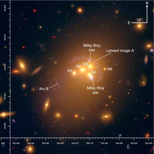
HST image of galaxy cluster Abell 3827, showing the F160W (red), F606W (green) and F336W (blue) bands. The colour scale is logarithmic. Labels show the four bright (plus one faint) central galaxies, foreground stars and background lensed galaxies. An object previously referred to as N.5 is actually a star. All these identifications are confirmed spectroscopically.
VLT spectroscopy
We first obtained spectroscopy across the cluster core using the VLT/VIMOS integrated field unit (IFU; Le Fèvre et al. 2003, 2013), programme 093.A-0237. Total exposure times were 6 h in the HR-blue filter (spanning a wavelength range 370–535 nm with spectral resolution λ/Δλ = 200) during 2014 July and 5 h in the MR-orange filter (490–1015 nm, with λ/Δλ = 1100) during 2014 August. All observations were obtained in photometric conditions and <0.6 arcsec seeing, using the 27 arcsec × 27 arcsec field of view; in this configuration, each pixel is 0.66 arcsec on a side.
Since the cluster core is high surface brightness across the entire VIMOS field of view, we interspersed every three exposures on target with one offset by ∼2 arcmin to record (and subtract) the sky background. The three on-source exposures were dithered by 1.3 arcsec (2 pixels) to account for bad fibres and cosmetics.
To reduce the raw data, we used the VIMOS esorex pipeline, which extracts the fibres, wavelength calibrates and flat-fields the data, and forms the data cube. We used the temporally adjacent sky exposure to perform sky subtraction (on a quadrant-by-quadrant basis), then mosaicked all of the exposures using a clipped average (using the bright stars to measure the relative offsets between cubes). We constructed (wavelength collapsed) continuum images from the cubes and aligned the cube to the HST imaging, then extracted spectra for each of the continuum sources. To search for emission from the strong lensing features, we applied a mask to the cube and extracted both one- and two-dimensional spectra. Due to the different resolutions of the HR-blue and MR-orange observations, we analysed the final two data cubes separately, but overall they provide a continuous wavelength coverage from 370 to 1015 nm. This is perfectly sufficient for our analysis of the cluster light.
The lensed galaxy threaded through the cluster core (labelled A in Fig. 1) was originally identified in Gemini imaging by Carrasco et al. (2010), who also used long-slit Gemini spectroscopy to obtain a redshift z = 0.204. However, our IFU spectroscopy did not confirm this. We instead found only one bright emission line at 835.5 nm, which is not associated with lines at the foreground cluster redshift and whose 2D morphology traces the lensed image. The emission line could have been Hα at z ≈ 0.27 or [O ii] at z ≈ 1.24 – but the low resolution and signal to noise of the VIMOS data precluded robust identification (the lack of other features, such as [N ii] λ6853 for z = 0.27 or [O iii] λ5007 for z = 1.24 may have been due to low metallicity and / or low signal-to-noise in the lines). Moreover, the flat-field (in)stability in VIMOS data left strong residuals after subtracting foreground emission from the cluster galaxies. In particular, this made it difficult to robustly determine the morphology of the arc near N.1, and — as we shall see in Section 4.2 — this provides the most diagnostic power in the lens modelling.
To confirm the redshift of lensed system A, and to measure its morphology around N.1, we observed the cluster core with the VLT Multi-Unit Spectroscopic Explorer (MUSE) IFU spectrograph (Bacon et al. 2010) during Director's Discretionary Time in 2014 December, programme 294.A-5014. The awarded exposure time of 1 h was split in to 3 × 1200 s exposures, which were dithered by ∼10 arcsec to account for cosmic rays and defects. These observations were taken in dark time, <0.7 arcsec V band seeing and good atmospheric transparency. We stacked these with an extra 1200 s exposure that was taken in good seeing during twilight, which marginally improves the signal to noise. MUSE has a larger 1 arcmin × 1 arcmin field of view and excellent flat-field stability, so no extra sky exposures were required. The data were reduced using v1.0 of the esorex pipeline, which extracts the spectra, wavelength calibrates, flat-fields the data and forms the data cube. These were registered and stacked using the exp_combine routine. The (much) higher throughput and higher spectra resolution (λ/Δλ = 3000) of MUSE yielded greatly improved signal to noise in both continuum and emission lines (see Appendix A for a comparison). For all our analysis of the background sources, we therefore use only the MUSE data.
In lensed system A, the MUSE data resolved the 835.5 nm emission line as the [O ii] λ3726.8, 3729.2 doublet at redshift zA = 1.24145 ± 0.00002, confirmed by the additional identification of Mg ii absorption at 627.0 nm (Fig. 2). The MUSE data also allowed a much improved continuum image to be constructed around the [O ii] emission, then subtracted to leave a higher fidelity [O ii] narrow-band image (Fig. 3).
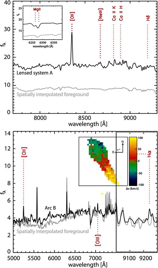
Observed spectra at the locations of background galaxies A (top panel) and B (bottom panel), smoothed for clarity with a Gaussian of width 5 Å. In both cases, the grey line shows the spectrum of nearby emission from the foreground cluster, spatially interpolated to the position of the background galaxy. The coloured insert shows galaxy B's 2D velocity field in a 6 arcsec × 6 arcsec region, for all IFU pixels where Hα emission is detected at signal to noise >4. It indicates a rotationally supported disc.
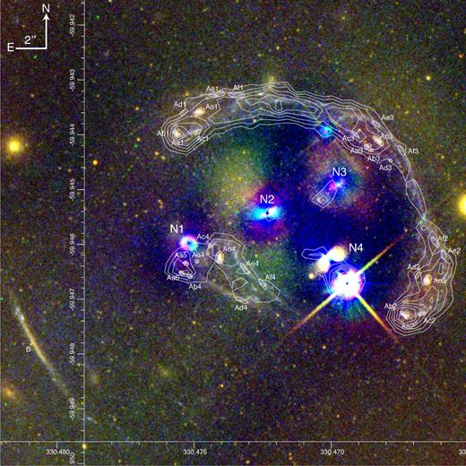
HST image of the core of Abell 3827, with light from the four bright galaxies subtracted to reveal the background lens system. Colours show the F814W (red), F606W (green) and F336W (blue) bands, and the colour scale is square root. Linearly spaced contours show line emission at 835.5 nm from VLT / MUSE integral field spectroscopy. Residual emission near galaxies N.3 and N.4 may be a demagnified fifth image or merely imperfect foreground subtraction, so we do not use it in our analysis.
For arc B, the MUSE data confirms Carrasco et al. (2010)'s Gemini long-slit redshift, finding zB = 0.4082 ± 0.0001 at the centre of the arc. Two blue knots at the north end dominate the [O ii] and [O iii] emission, but Hα emission is visible across its entire length (all three features are at the same redshift). A 2D map of the best-fitting wavelength of the Hα emission shows a monotonic velocity gradient of ∼200 km s−1 from north to south (Fig. 2). We are confident that no multiple images are present, having inspected both the HST imaging and narrow-band images created from the MUSE data at the wavelengths of the emission lines.
ANALYSIS
Modelling the cluster light distribution
It is apparent from the high-resolution imaging (Fig. 1) and our IFU spectroscopy that Abell 3827 contains four bright central galaxies, N.1–N.4. The object labelled N.5 by Carrasco et al. (2010) is a Milky Way star: it is a point source in the HST imaging, and its spectrum contains z = 0 Ca ii H and K absorption lines that are not present in adjacent sources. Their spectroscopy of N.5 was probably contaminated by the nearby bright cluster galaxies and diffuse intracluster light. On the other hand, the westernmost object that Carrasco et al. (2010) identified as a star, is actually a faint cluster member galaxy at z = 0.1000 ± 0.0002. To avoid confusion, we denote this galaxy N.6.
In the optical HST imaging, we use galfit (Peng et al. 2010) to simultaneously fit the light distribution from the four bright galaxies and the two stars. Most galaxies are well fitted by a single component model with a Sérsic profile, although a double-component model using two Sérsic profiles (with the same centre) is preferred for galaxy N.3 (and galaxy N.2 in the F814W band). Positions in the F814W band are listed in Table 1; those in F606W are consistent within 0.006 arcsec for N.1–3 and, 0.061 arcsec for N.4, due to its proximity to a bright star. To model emission from the stars, we shift and rescale an isolated star in the same image. The best-fitting galaxy fluxes do not depend significantly upon the choice of isolated star or the alternative use of a tinytim model star (Rhodes et al. 2007; Krist, Hook & Stoehr 2011). The photometric errors are dominated by our assumption of analytic functions to fit the light profiles. The fluxes are likely to be an upper limit because they are computed by integrating these analytic functions to infinite radius, and may also include a component of diffuse intracluster light.
Total integrated flux of the bright central galaxies, and their derived stellar masses. In both HST/ACS bands (independently), we use galfit (Peng et al. 2010) to simultaneously fit the emission from all four galaxies. Dagger denote that a two-component (co-centred) Sérsic model was preferred. Positions are listed from the F814W band, and are consistent with those from the F606W band. Stellar masses M* interpret the single-band AB magnitude flux via the models of Bruzual & Charlot (2003), assuming a Chabrier (2003) IMF, solar metallicity, and formation redshift zf = 3. Redshifts, 3σ upper limits on Hα flux (interpreted as limits on SFR via Kennicutt 1998, also converted to a Chabrier 2003 IMF), and stellar velocity dispersions are measured from VLT spectroscopy.
| F814W band | F606W band | Hα flux | SFR | |$\sigma _\mathrm{v}^*$| | ||||||
|---|---|---|---|---|---|---|---|---|---|---|
| RA | Dec | z | (mag) | M* (M⊙) | mag | M* (M⊙) | (erg s−1 cm−2) | (M⊙ yr−1) | (km s−1) | |
| N.1 | 330.475 18 | −59.945 997 | 0.098 91 ± 0.000 32 | 16.86 | 1.04 × 10¹¹ | 17.52 | 1.00 × 10¹¹ | <6.04 × 10⁻¹⁶ | <0.14 | 332 |
| N.2 | 330.472 33 | −59.945 439 | 0.099 28 ± 0.000 17 | 15.74† | 2.92 × 10¹¹ | 16.55 | 2.46 × 10¹¹ | <2.59 × 10⁻¹⁶ | <0.06 | 377 |
| N.3 | 330.469 78 | −59.944 903 | 0.099 73 ± 0.000 16 | 15.69† | 3.06 × 10¹¹ | 16.42† | 2.77 × 10¹¹ | <6.31 × 10⁻¹⁶ | <0.14 | 326 |
| N.4 | 330.469 99 | −59.946 322 | 0.096 36 ± 0.000 26 | 16.18 | 1.94 × 10¹¹ | 16.73 | 2.08 × 10¹¹ | <1.57 × 10⁻¹⁵ | <0.26 | 192 |
In the VLT/VIMOS spectroscopy, we measure the redshift of galaxies N.1–N.4 and N.6 by fitting a Gaussian to the H, K and G-band absorption features. None of the cluster galaxies exhibits Hα line emission, although we attempt to fit a Gaussian at its redshifted wavelength to obtain 3σ upper limits on the Hα flux. To measure the stellar velocity dispersion, we cross-correlate our spectra with broadened stellar templates from Vazedkis (1999). These measurements are presented in Table 1.
Strong lens identifications
Fig. 3 presents a multicolour image of Abell 3827, after subtracting the best-fitting model of optical emission from the optical HST bands to reveal the morphology of the gravitationally lensed system. In the UV HST imaging, the contrast between cluster member galaxies and the background lens system is much lower, so we do not fit and subtract the foreground flux.
Lensed image A is an almost face-on spiral galaxy, with a bulge and many resolved knots of star formation that can all be used as independent lensed sources. The association of knots between multiple images is not perfectly clear, due to the bright intracluster light and a surprising density of point sources, particularly near galaxy N.1; we present the most likely identifications in Table 2, but analyse alternative configurations in Appendix B. Contours in Fig. 3 show a (continuum subtracted) narrow-band image created by subtracting continuum emission from each spatial pixel (fitted using a low-order polynomial over the wavelength range 830–840 nm) then collapsing the MUSE IFU data cube over ±300 km s−1 from the peak of the emission. The 2D map of this line emission matches precisely the lensed galaxy's broad-band morphology. Variations in the intensity of the line emission can be explained by lensing magnification. According to our fiducial Lenstool model (see Section 4.2.2), the magnification at the position of the bulge images, and variation across the spiral is |$1.29^{+0.10}_{-0.15}$| for image 1, |$0.95^{+0.06}_{-0.03}$| for images 2 and 3, but |$1.62^{+0.43}_{-0.28}$| for image 4 (with the magnification greatest near galaxy N.1).
Locations of multiply imaged systems. Images Ao.n are the bulge, and images A[a–f].n are knots of star formation in the spiral arms. Index n is sorted in order of arrival time according to our fiducial model (see Table 3). Columns denote the ID and position of the image, its major and minor axes, and the angle of its major axis on the sky, anticlockwise from west.
| Name | RA | Dec | Major (arcsec) | Minor (arcsec) | Angle |
|---|---|---|---|---|---|
| Ao.1 | 330.474 79 | −59.943 580 | 0.33 | 0.22 | 25° |
| Ao.2 | 330.466 49 | −59.946 650 | 0.35 | 0.23 | 75° |
| Ao.3 | 330.468 28 | −59.944 112 | 0.43 | 0.16 | 140° |
| Ao.4 | 330.474 07 | −59.946 239 | 0.39 | 0.25 | 85° |
| Aa.1 | 330.475 59 | −59.944 009 | 0.16 | 0.14 | 151° |
| Aa.2 | 330.467 25 | −59.947 321 | 0.16 | 0.14 | 140° |
| Aa.3 | 330.468 71 | −59.944 215 | 0.16 | 0.14 | 131° |
| Aa.4 | 330.474 89 | −59.946 312 | 0.12 | 0.10 | 54° |
| Aa.5 | 330.475 29 | −59.946 349 | 0.18 | 0.13 | 150° |
| Aa.6 | 330.475 46 | −59.946 523 | 0.18 | 0.12 | 150° |
| Ab.1 | 330.475 71 | −59.943 954 | 0.11 | 0.09 | 131° |
| Ab.2 | 330.467 41 | −59.947 260 | 0.14 | 0.11 | 131° |
| Ab.3 | 330.468 52 | −59.944 283 | 0.11 | 0.09 | 131° |
| Ab.4 | 330.475 15 | −59.946 584 | 0.18 | 0.12 | 150° |
| Ac.1 | 330.474 89 | −59.943 958 | 0.25 | 0.13 | 41° |
| Ac.2 | 330.466 69 | −59.947 267 | 0.25 | 0.08 | 20° |
| Ac.3 | 330.469 12 | −59.943 994 | 0.30 | 0.08 | 140° |
| Ac.4 | 330.474 41 | −59.946 030 | 0.12 | 0.08 | 220° |
| Ad.1 | 330.475 37 | −59.943 594 | 0.28 | 0.13 | 40° |
| Ad.2 | 330.466 85 | −59.946 564 | 0.26 | 0.10 | 60° |
| Ad.3 | 330.467 84 | −59.944 468 | 0.12 | 0.08 | 157° |
| Ad.4 | 330.473 26 | −59.947 020 | 0.42 | 0.13 | 160° |
| Ae.1 | 330.473 45 | −59.943 276 | 0.53 | 0.17 | 178° |
| Ae.2 | 330.465 90 | −59.946 186 | 0.28 | 0.16 | 100° |
| Ae.3 | 330.468 37 | −59.943 805 | 0.30 | 0.13 | 150° |
| Ae.4 | 330.473 15 | −59.946 447 | 0.42 | 0.13 | 130° |
| Af.1 | 330.474 17 | −59.943 267 | 0.52 | 0.15 | 10° |
| Af.2 | 330.466 21 | −59.945961 | 0.39 | 0.16 | 130° |
| Af.3 | 330.467 45 | −59.944 289 | 0.37 | 0.13 | 123° |
| Af.4 | 330.472 49 | −59.946 730 | 0.42 | 0.13 | 130° |
The 835.5 nm emission near the galaxies N.4 and N.3 is possibly a demagnified image of bulge Ao and knot Aa. A demagnified image of the bulge is robustly predicted between N.2 and N.4, although our fiducial lenstool model places it closer to N.2 at (330.471 35, −59.945 850). Models allowing a demagnified image of Aa stretched towards N.3 are possible, but at lower likelihood, and (for reasonable positions of the cluster-scale halo) this would be in addition to a demagnified image between N.2 and N.4. Since these identifications are not robust with current data, and could be merely imperfect foreground subtraction near the bright cluster galaxies, we exclude them from our strong lensing analysis
Arc B would be difficult to interpret as a strong lens, as previously suggested, because it is at lower redshift than system A but greater projected distance from the lens (whereas Einstein radius should increase with redshift). Instead, its constant velocity gradient suggests that is merely an edge-on spiral galaxy, aligned by chance at a tangential angle to the cluster, elongated and flexed (our fiducial lenstool model predicts shear γ = 0.20 ± 0.01) but only singly imaged. The two knots of star formation at its north end further enhance its visual appearance of curvature. This is consistent with the absence of observed counterpart images, and the lack of fold structure in its 2D velocity field. We therefore exclude arc B from our strong lensing analysis.
Modelling the cluster mass distribution
To model the strong gravitational lens system, we use two independent software packages: grale (Liesenborgs, De Rijcke & Dejonghe 2006) and lenstool (Jullo et al. 2007). The two packages make very different assumptions. grale models the mass distribution using a free-form grid, in which the projected density at each pixel is individually constrained and individually adjustable; lenstool interpolates a parametric model built from a relatively small number of components, each of which has a shape that matches the typical shapes of clusters. The two packages also exploit slightly different features of the input data. For example, both methods match the position of multiply-imaged systems, but grale can also match their shape, and use the absence of counter images where none are observed; while lenstool can expoit the symmetries of great arcs.
GRALE
grale is a free-form, adaptive grid method that uses a genetic algorithm to iteratively refine the mass map solution (Liesenborgs et al. 2006, 2007, 2008a,b, 2009; Liesenborgs & De Rijcke 2012). We work within a 50 arcsec × 50 arcsec reconstruction region, centred on (330.470 43, − 59.945 804). An initial coarse resolution grid is populated with a basis set; in this work we use projected Plummer density profiles (Plummer 1911; Dejonghe 1987). A uniform mass sheet covering the whole modelling region can also be added to supplement the basis set. As the code runs, the more dense regions are resolved with a finer grid, with each cell having a Plummer with a proportionate width. The code is started with an initial set of trial solutions. These solutions, as well as all the later evolved ones are evaluated for genetic fitness, and the fit ones are cloned, combined and mutated. The resolution is determined by the number of Plummers used. The initial coarse resolution grid is refined nine times, allowing for more detail in the reconstruction; the best map is selected based on the fitness measure. The final map consists of a superposition of a mass sheet and many Plummers, typically a few hundred to a thousand, each with its own size and weight, determined by the genetic algorithm. Note that adopting a specific (Plummer) density profile for our basis set does not at all restrict the profile shapes of the mass clumps in the mass maps.
We use two types of fitness measures in this work. (a) Image positions. A successful mass map would lens image-plane images of the same source back to the same source location and shape. We take into account the position, shape, and angular extent of all the images in Table 2, by representing each image as a collection of points that define an area. A mass map has a greater fitness measure if the images have a greater fractional area overlap in the source plane. This ensures against over-focusing, or overmagnifying images, which plagued some of the early lens reconstruction methods. (b) Null space. Regions of the image plane that definitely do not contain any lensed features belong to the null space. Each source has its own null space. Typically, a null space is all of the image plane, with ‘holes’ for the observed images, and suspected counter images, if any. The product of these two fitness measures is used to select the best map in each reconstruction.
All lensed images in this cluster arise from extended sources (star formation knots within a galaxy). Because of that it is hard to identify the centre of each image to a precision comparable to HST resolution. The 0.3 arcsec–0.6 arcsec extent of grale points representing some image will be, approximately, the lower bound on the lens plane rms between the observed and predicted images.
We run 20 mass reconstructions for each image configuration (a limit set by computational time constraints), and the maps that are presented here are the averages of these. The full range of the recovered maps provides an estimate of the statistical error in the mass maps.
LENSTOOL
lenstool is a parametric method that uses a Markov Chain Monte Carlo (MCMC) fit with a comparatively smaller number of mass peaks, but which are free to move and change shape. We construct our mass model using one dual Pseudo Isothermal Elliptical (Limousin, Kneib & Natarajan 2005; Elíasdóttir et al. 2007) halo for the overall cluster, plus a smaller Pseudo Isothermal Elliptical halo for each galaxy N.1–4 and N.6. Each halo is characterized by a position (x, y), velocity dispersion σv, ellipticity e, and truncation radius rcut; the cluster halo is also allowed to have a non-zero core radius rcore. We set the following priors on the cluster halo: e < 0.75, rcore < 4 arcsec, and the position has Gaussian probability with width σ = 2 arcsec centred on N.2. For the galaxy haloes, we set a prior e < 0.45. The position of N.1 is of particular scientific interest, and will be well constrained because it is surrounded by strong lens images, so to avoid any bias, we set a prior that is flat within −5 arcsec < x < 3 arcsec and −3 arcsec < y < 3 arcsec of the optical emission. The position of N.2–N.4 will be less well constrained, so we set Gaussian priors1 with width σ = 0.5 arcsec, centred on their optical emission. The parameters of N.6 are poorly constrained, because it is faint and far from the strong lens systems, so we fix its position to that of its optical emission, and fix e = 0 to reduce the search dimensionality. The strong lensing data alone provide no constraints on the outer regions of the mass distribution, so we manually fix rcut = 1000 arcsec for the cluster halo, and rcut = 100 arcsec for the galaxy haloes, well outside any region of influence.
As constraints, we use the positions of all multiple images in Table 2 and, following additional symmetries of the image, require the zA = 1.24 critical curve to pass through (330.471 13, −59.943 529) and (330.466 77, −59.945 195) perpendicular to an angle of 175° and 110°, respectively. These are indicated in the bottom panel of Fig. 4. We then optimize the model in the image plane using an MCMC search with parameter bayesrate = 0.1 (which allows the posterior to be well explored during burn-in, before converging to the best-fitting solution; for more details, see Kneib et al. 1996; Smith et al. 2005; Jauzac et al. 2014a). We assume an error of 0.2 arcsec (68 per cent CL) on every position. This choice merely rescales the posterior. If we instead assume an error of 0.273 arcsec, the model achieves reduced χ2/dof = 1.
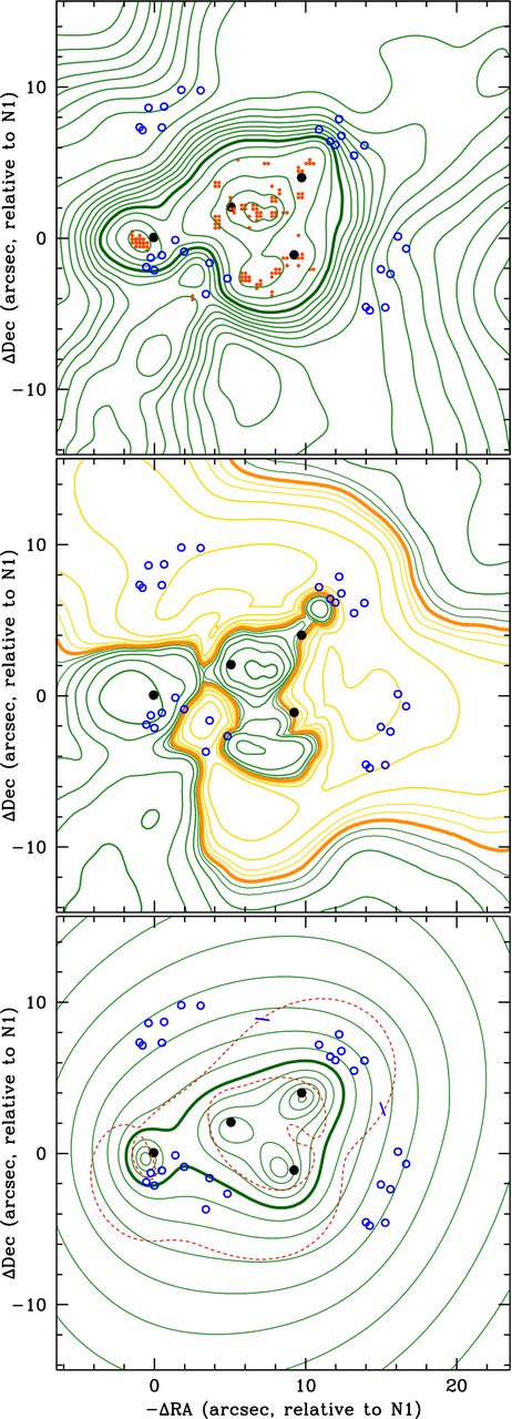
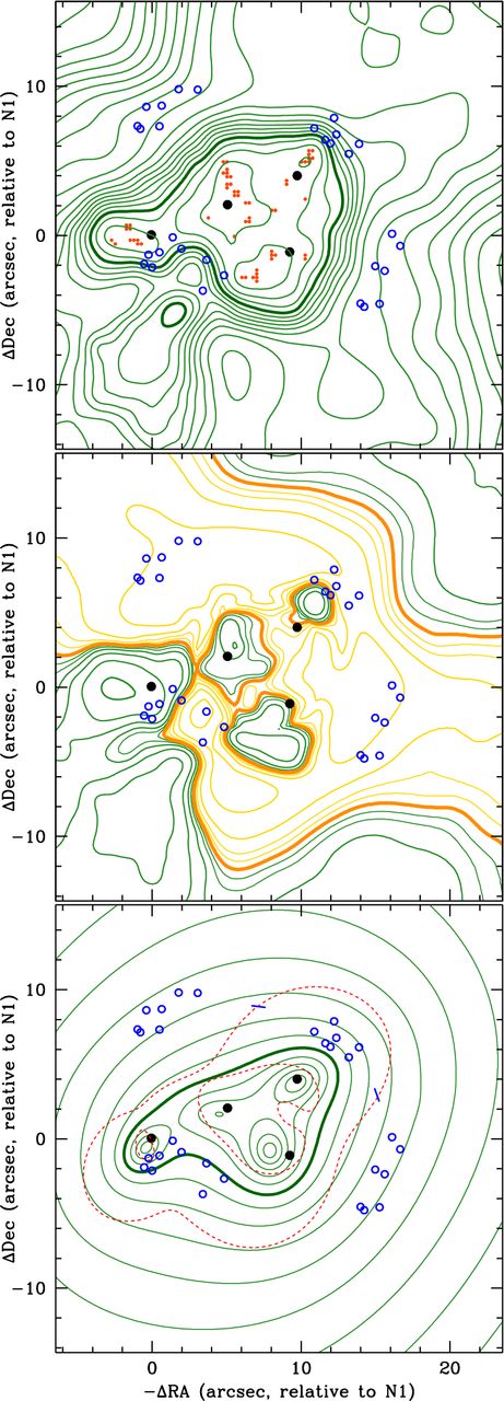
Top panel: map of total mass in the cluster core, reconstructed using grale. Green contours show the projected mass density, spaced logarithmically by a factor of 1.15; the thick contour shows convergence κ = 1 for zcℓ = 0.099 and zA = 1.24 (Σcrit = 1.03 g cm−2). Red dots show local maxima in individual realizations of the mass map. Black dots show cluster ellipticals N.1–N.4. Blue circles show the lensed images. Middle panel: mass after subtracting a smooth cluster-scale halo to highlight substructure. The thick contour is at Δκ = 0. The green (positive) and yellow (negative) contours are at Δκ = ±0.025, ±0.05, ±0.1, ±0.2,.... Bottom panel: total mass, as in the top panel but reconstructed via lenstool. The red dashes show the zA = 1.24 critical curve.
RESULTS
Stellar mass
Spectroscopic redshifts of N.1–N.4 and N.6 confirm that they are all zcℓ ≈ 0.099 cluster members. Notably, N.1–N.3 are at essentially the same redshift as each other (which is consistent with the mean redshift of all known member galaxies), and are projected along a straight line. One the other hand, N.4 has a relative line-of-sight velocity ∼900 km s−1.
In Table 1, we interpret the galaxies’ integrated broad-band fluxes (in individual filters) as stellar masses M* via the models of Bruzual & Charlot (2003), assuming a Chabrier (2003) initial mass function (IMF), solar metallicity, and formation redshift zf = 3. The inferred stellar mass of N.1 is surprisingly low compared to its stellar velocity dispersion, but this could be because it is furthest from the cluster core, so its measured flux contains the least contamination from intracluster light.
We also interpret the 3σ upper limits on the Hα flux as star formation rate (SFR), following Kennicutt (1998) relations converted to a Chabrier (2003) IMF. The red and dead ellipticals exhibit effectively zero star formation, consistent with their faint UV broad-band fluxes.
Total mass distribution
GRALE
The grale reconstruction of the projected mass distribution within the central 30 arcsec × 30 arcsec of the 50 arcsec × 50 arcsec fitted region is shown in the top panel of Fig. 4. The mean rms offset of observed lens images from their predicted positions in the image plane is 〈rmsi〉 = 0.34 arcsec, but this value is inflated by the size of the input images, as explained in Section 3.3.1.
The mass distribution peaks at (330.47068, −59.945513), i.e. (8.15 arcsec, 1.73 arcsec) or r = 8.33 arcsec from galaxy N.1. The total mass of the cluster core inside a cylinder with this radius and centred on the mass peak is Mcℓ = 3.58 × 10¹² M⊙. The typical fractional error in surface mass density in the central region is ∼15 per cent. The total mass projected within 1.5 arcsec = 2.7 kpc of galaxies N.1–4 is 1.63, 2.02, 1.70 and 1.67 × 10¹¹ M⊙, respectively.
To highlight the position of substructures, the red dots in the top panel of Fig. 4 show the local maxima in each of the individual, statistically independent realizations of the mass map (within the central κ = 1 contour only), and the middle panel of Fig. 4 shows the mean map after subtracting a smooth, cluster-scale halo. The cluster-scale halo used is centred on the peak density, has constant projected density inside a core of radius 4.4 arcsec = 8.0 kpc, and a projected density profile ρ2D(r) ∝ r−1.3 outside this core.
The most robustly constrained region of interest is near galaxy N.1, owing to the proximity of several lensed images. Local peaks in individual realizations of the mass map form a tight cluster 1.01 arcsec ± 0.39 east–southeast of the peak of optical emission, implying that the offset is significant at the 2.6σ level. The mass within 1.5 arcsec of this location is 1.66 × 10¹¹ M⊙.
Galaxy N.3 is next nearest to gravitationally lensed images. The closest local mass peak is frequently 1–2 arcsec north-west of the optical emission, and the mass within 1.5 arcsec of this location is 1.38 × 10¹¹ M⊙. Statistically significant structure is apparent in the mean mass map, but its presence is less robust than for N.1. It may be interesting that galaxies N.1–3, the mass peaks closest to N.1 and N.3, and the cluster's large-scale diffuse light all lie close to a straight line. Infall from preferred directions along filaments is expected (e.g. Schaye et al. 2015) – although orbits of galaxies do not generally stay radial this far from the virial radius, so it may also be coincidence. Galaxy N.4 has no local mass peak in many realizations of the reconstruction; the closest set of peaks is offset ∼3 arcsec to the south-east. However, the region around N.4 is not as well constrained by nearby lensed images, and Appendix B shows that the distribution of surrounding mass is sensitive to the assumed identification of strong lens images. The position of the mass associated with galaxy N.2 is difficult to disentangle from that of the cluster-scale halo.
LENSTOOL
Best-fitting parameters for the fiducial mass model are listed in Table 3, and the corresponding mass map is shown in the bottom panel of Fig. 4 (it is uninformative to subtract the cluster scale halo, as its core is flatter than the cuspy galaxies, so does not visually affect their position). The mean rms offset of observed lens images from their predicted positions in the image plane is 〈rmsi〉 = 0.26 arcsec (41 per cent of which is contributed by systems Ae and Af, whose observed position in some multiple images is indeed the least certain). With the assumed 0.2 arcsec errors on observed positions, the model achieves χ2/dof = 49.3/23, and Bayesian evidence log10(E) = −26.4. Some of the lenstool MCMC samples predict fifth and sixth images of knot Ac to the east of Aa.5 and Aa.6, which are indeed faintly visible as the continuation of image A's ring.
Parameters of the best-fitting, fiducial mass model constructed by lenstool. Positions are relative to the peak of light emission, except for the cluster-scale halo, whose position is relative to the peak of emission from galaxy N.1. Quantities in square brackets are not fitted. Errors on other quantities show 68 per cent statistical confidence limits due to uncertainty in the lensed image positions, marginalizing over uncertainty in all other parameters.
| σv (km s−1) | x (arcsec ) | y (arcsec ) | e | θ (°) | rcore (arcsec) | 〈rmsi〉 (arcsec ) | χ2/dof | log10(E) | |
|---|---|---|---|---|---|---|---|---|---|
| Fiducial model: | 0.26 | 49.3/23 | −26.4 | ||||||
| N.1 | 190|$^{+8}_{-12}$| | −0.61|$^{+0.14}_{-0.12}$| | −0.46|$^{+0.20}_{-0.14}$| | 0.25|$^{+0.15}_{-0.04}$| | 101|$^{+22}_{-22}$| | [→0] | |||
| N.2 | 219|$^{+18}_{-38}$| | −0.13|$^{+0.28}_{-0.46}$| | −0.48|$^{+0.30}_{-0.30}$| | 0.09|$^{+0.12}_{-0.09}$| | 174|$^{+22}_{-37}$| | [→0] | |||
| N.3 | 254|$^{+17}_{-14}$| | 0.09|$^{+0.25}_{-0.25}$| | −0.36|$^{+0.18}_{-0.29}$| | 0.25|$^{+0.04}_{-0.10}$| | 30|$^{+11}_{-13}$| | [→0] | |||
| N.4 | 235|$^{+20}_{-34}$| | −0.99|$^{+0.39}_{-0.34}$| | −0.01|$^{+0.35}_{-0.27}$| | 0.19|$^{+0.12}_{-0.09}$| | 121|$^{+22}_{-54}$| | [→0] | |||
| N.6 | 18|$^{+44}_{-1}$| | [0] | [0] | [0] | [0] | [→0] | |||
| Cluster | 620|$^{+101}_{-58}$| | 6.18|$^{+1.33}_{-1.04}$| | 2.30|$^{+1.86}_{-1.51}$| | 0.70|$^{+0.01}_{-0.24}$| | 61|$^{+3}_{-4}$| | 30.12|$^{+9.23}_{-6.43}$| |
The total mass projected within r = 8.33 arcsec of (330.470 68, −59.945 513) is Mcℓ = 3.49 × 10¹² M⊙. The total mass within 1.5 arcsec of galaxies N.1–4 is 0.65, 1.20, 1.48 and 1.83 × 10¹¹ M⊙, respectively. These numbers include a contribution from the cluster-scale halo, and are most useful for comparison to the grale results. Integrating the individual components of the mass model analytically within a 1.5 arcsec radius, excluding the cluster halo, yields masses of 0.72, 0.95, 1.28 and 1.10 × 10¹¹ M⊙ (see equation 9 of Limousin et al. 2005). The mass associated with N.1 increases slightly in this calculation because these measurements are centred on the mass peaks. The 68 per cent confidence limits on all of these masses, obtained by propagating the statistical uncertainty (only) in the observed image positions through the MCMC sampler, are approximately 1 per cent.
The mass associated with galaxy N.1 is offset by |$0.76^{+0.13}_{-0.16}\,{\rm arcsec}$| from the peak of its light emission.2 The 68 per cent confidence limit, again obtained from the MCMC samples, includes only statistical uncertainty propagated from that in the observed image positions. To estimate the additional uncertainty (bias) caused by the relative inflexibility of lenstool's parametric model to represent a complex mass distribution, we retry the optimisation using two alternative model configurations.
Refitting the data using a model with a second cluster-scale halo achieves 〈rmsi〉 = 0.25 arcsec, although with worse χ2/dof = 48.5/17, and log10(E) = −28.0. In this model, the first cluster halo remains between N.2 and N.3, and the second cluster halo appears between N.3 and N.4, whose masses are reduced by ∼45 per cent. The mass associated with galaxy N.1 moves to |$(-0.68^{+0.13}_{-0.12}\,{\rm arcsec} ,\,-0.25^{+0.19}_{-0.12}\,{\rm arcsec})$|. This 0.22 arcsec shift relative to the fiducial reconstruction provides one estimate of model-induced bias.
Secondly, we can reuse the fiducial model to perform an MCMC fit to a mass distribution that has a similar configuration to the real distribution but is not impeded by the parametric limitations of lenstool. We generate four, slightly different realizations of mock data by raytracing the positions of each lensed image (e.g. A[a–f].1) through the fiducial model to the source plane, then back to (multiple locations in) the image plane. In this mock data, the true position of the mass is known, and can be represented perfectly by lenstool. We perform four independent fits, centring the priors around the true positions of the mass. The mean spurious offset of N.1 is 0.55 arcsec ± 0.11, and the mean spurious offsets of N.2–4 are 0.55 arcsec ± 0.09. Comparing this to the total ∼0.76 arcsec offsets in the real fit therefore suggests a similar ∼0.21 arcsec budget for model-induced bias.
The mean offset of N.2–4 (with the observed constraints) is 0.62 arcsec, which could be interpreted to imply a characteristic error on N.1 of this order. However, these are measured with a prior, and their uncertainty is much greater than that of N.1 because those galaxies happen to be much farther from strongly lensed systems – and, in the case of N.2, because of degeneracy with the position of the cluster-scale halo. Contrary to the results from grale, the mass associated with galaxy N.3 is coincident with the position of its light emission within measurement error; the mass within 1.5 arcsec of grale's offset peak is a lower 1.07 × 10¹¹ M⊙. The mass associated with N.4 is offset at only marginal statistical significance but, intriguingly, the offset is in the same direction as that measured by grale.
INTERPRETATION
We have modelled the distribution of mass in the cluster using two independent approaches: free-form grale and parametric lenstool. The general agreement between methods is remarkable, both in terms of total mass and many details.
Using a different set of strong lens image assignments (see Appendix B), we recover the 6 kpc offset and correspondingly larger cross-section of Williams & Saha (2011). These image assignments are now ruled out by our new IFU spectroscopy, which unambiguously traces the morphology of the lens, even through foreground emission and point sources in the broad-band imaging.
We have also measured the mass-to-light ratios of the four central galaxies. Each of them retains an associated massive halo. There is no conclusive evidence to suggest that any of them are more stripped than the others; if anything, the stellar mass of N.1 is marginally lower than expected, compared to both the stellar and dark matter measurements of velocity dispersion. This is the opposite of behaviour expected if the dark matter associated with N.1 is being stripped.
We have not yet attempted to measure any truncation of the galaxy haloes, like Natarajan et al. (2009). That measurement will be improved by combining our current measurements of strong lensing with spatially extended measurements of weak lensing and flexion currently in preparation, plus multi-object spectroscopic data of member galaxies outside the cluster core.
CONCLUSIONS
We have presented new HST imaging and VLT integrated field spectroscopy of galaxy cluster Abell 3827. This is a uniquely interesting system for two reasons. First, it contains an unusually corrugated light distribution, with four almost equally bright central galaxies (not five, as previously thought, because one is a foreground star) within the central 10 kpc radius. Secondly, a gravitationally lensed image of a complex spiral galaxy is fortuitously threaded between the galaxies, allowing the distribution of their total mass to be mapped. Because of the cluster's z ∼ 0.1 proximity, this can be achieved with high spatial precision. We expect this data will be useful beyond this first paper, for several investigations of late-time dark matter dynamics in the poorly-studied (yet theoretically contentious) regime of cluster cores.
We have investigated the possible stripping or deceleration of dark matter associated with the infalling galaxies. Most interestingly, combining two independent mass mapping algorithms, we find a |$1.62^{+0.47}_{-0.49}$| kpc offset (i.e. 3.3σ significance) between total mass and luminous mass in the best-constrained galaxy, including statistical error and sources of systematic error related to the data analysis. Such an offset does not exist in isolated field galaxies (or it would have been easily detected via strong lensing of quasars). If interpreted in terms of a drag force caused by weak self-interactions between dark matter particles, this suggests a particle cross-section σ/m ∼ (1.7 ± 0.7) × 10−4 cm2 g−1. However, the small absolute offset <2 kpc might be caused by astrophysical effects such as dynamical friction, and it is difficult to conclude definitively that real dark matter is behaving differently to cold dark matter. Detailed hydrodynamical simulations of galaxy infall, incorporating dark matter physics beyond the standard model, are needed to predict its behaviour within a cluster environment, and to more accurately interpret high-precision observations.
The authors are pleased to thank Jay Anderson for advice with CTI correction for HST/WFC3, Jean-Paul Kneib for advice using lenstool, and the anonymous referee whose suggestions improved the manuscript. RM and TDK are supported by Royal Society University Research Fellowships. This work was supported by the Science and Technology Facilities Council (grant numbers ST/L00075X/1, ST/H005234/1 and ST/I001573/1) and the Leverhulme Trust (grant number PLP-2011-003). This research was carried out in part at the Jet Propulsion Laboratory, California Institute of Technology, under a contract with NASA.
Facilities: This paper uses data from observations GO-12817 (PI: R. Massey) with the NASA/ESA Hubble Space Telescope, obtained at the Space Telescope Science Institute, which is operated by AURA Inc, under NASA contract NAS 5-26555. This paper also uses data from observations made with ESO Telescopes at the La Silla Paranal Observatory under programmes 093.A-0237 and 294.A-5014 (PI: R. Massey). We thank the Director General for granting discretionary time, and Paranal Science Operations for running the observations. The lenstool analysis used the DiRAC Data Centric system at Durham University, operated by the Institute for Computational Cosmology on behalf of the STFC DiRAC HPC Facility (www.dirac.ac.uk). This equipment was funded by BIS National E-infrastructure capital grant ST/K00042X/1, STFC capital grant ST/H008519/1, and STFC DiRAC Operations grant ST/K003267/1 and Durham University. DiRAC is part of the National e-Infrastructure. LLRW would like to acknowledge the Minnesota Supercomputing Institute, without whose computational support grale work would not have been possible.
We check that the Gaussian priors do not bias the best-fitting position by shifting the priors to the peaks in the posterior and rerunning the analysis. Positions all move by less than 0.08 arcsec in x and y, indicating convergence to within statistical errors.
This remains as |$0.81^{+0.13}_{-0.12}$| arcsec even if 10 per cent of the mass (accounting for the stellar component) is forced to lie on the galaxy; the offset is necessary to ensure the observed multiplicity of Aa.5 and Aa.6.
Note that the pre-factor in equation 4 of Williams & Saha (2011) should be 6.0 × 10³ rather than 6.0 × 10⁴.
REFERENCES
APPENDIX A: COMPARISON OF VIMOS AND MUSE SPECTROSCOPY
Our IFU observations of the same (faint and highly elongated) source with both VLT/VIMOS (Le Fèvre et al. 2003) and VLT/MUSE (Bacon et al. 2010) provide an early opportunity to compare the practical performance of VLT's old and new spectrographs. As is apparent in Fig. A1, the throughput of MUSE is vastly greater, achieving higher signal to noise in a much shorter exposure time. Crucially for our purposes, the improved flat-field stability allows much cleaner foreground subtraction, revealing candidates for the demagnified fifth image near foreground galaxies N.3 and N.4. MUSE's higher spectral resolution and larger field of view are also responsible for two fortuitous discoveries: our identification of line emission in lensed galaxy A as the [Oii] doublet, which we had previously mistaken for Hα, and the identification of galaxy B as an edge-on spiral, which we had previously mistaken for a strong gravitational lensing arc. Availability of the new MUSE spectrograph has thus revolutionized our interpretation of this cluster.
![False-colour images of the cluster core, manufactured from the VLT/VIMOS and VLT/MUSE IFU 3D data cubes. The displayed region shows the full field of view of each instrument. Red, green and blue channels, respectively, correspond to a narrow-band [O ii] image (created as described in Section 3.2), Johnson I band and Johnson V band.](https://oup.silverchair-cdn.com/oup/backfile/Content_public/Journal/mnras/449/4/10.1093_mnras_stv467/1/m_stv467figa1.jpeg?Expires=1716430310&Signature=vDHEmbKsElxBwhuNUM6L0aqDkWXdTESdyuqkNDAvf67Z~N02sH3ky8fBZEZjug9F5AHN-fzSpoM3WLZgvr61PyEnwd-KjVbv-wUIWfmPNnD2Exwz7cGswbXopB8xLjBQ30KbRBMDhY8sYh1ahp2yj0JPrhsGiK~6Q5AHQt5rOJ2wrCeTtudbVyT9PQSwy95pPwK8tXgVyw5P62ALrduJwCdZ2Wd-gJ2wxtuy9HG0-8dScGBEBmw5RhXETsvyhBVOTQY0YxqHy3uoOiwAQvkBI2nQUI4lLDoAeaw84ZyjuVBofwRFyxqoT~1K6FaJx6xq-efnq6DeaMGt4QB40PrDOg__&Key-Pair-Id=APKAIE5G5CRDK6RD3PGA)
False-colour images of the cluster core, manufactured from the VLT/VIMOS and VLT/MUSE IFU 3D data cubes. The displayed region shows the full field of view of each instrument. Red, green and blue channels, respectively, correspond to a narrow-band [O ii] image (created as described in Section 3.2), Johnson I band and Johnson V band.
APPENDIX B: ALTERNATIVE LENSED IMAGE ASSOCIATIONS
To draw robust conclusions about any offsets between optical emission and associated dark matter, one needs to account for all sources of uncertainty in the mass models. Statistical uncertainties in the location of the mass peaks around galaxy N.1 are easily obtained. There are two types of additional uncertainties: those arising from the mass reconstruction methods, and those from the image identification. We explore the latter in this appendix, by considering two alternative image assignments (see Fig. B1).
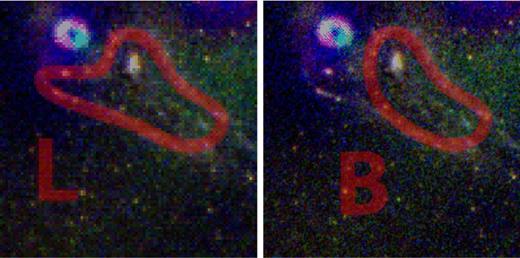
Two alternative configurations of lensed image associations near cluster galaxy N.1. There is a surprising high density of point sources, so it is not obvious which sources correspond to which lensed images. Configuration L is a small perturbation of the fiducial model in the main paper. Configuration B is based upon lentool's best-fitting mass model if no identifications are initially made in this region. However, it is at odds with narrow-band imaging of the source, created from line emission in our VLT IFU data (see Fig. 3).
In the body of this paper, we presented a fiducial model using what we believe to be the correct associations – based on the surface brightness, colours and sizes of the knots in HST imaging, and the extended distribution of [O ii] emission in IFU spectroscopy. The only questionable region is around N.1; the other image assignments are secure (though the exact locations of some faint extended images, like Ae and Af, are uncertain to within a few tenths of an arcsecond). All the image assignment schemes, we have tried produce a common elongation of the mass distribution along the north-west to south-east axis, and a statistically significant offset between the light and mass of N.1, using both grale and lenstool. However, the amount and the morphology of the offset differs.
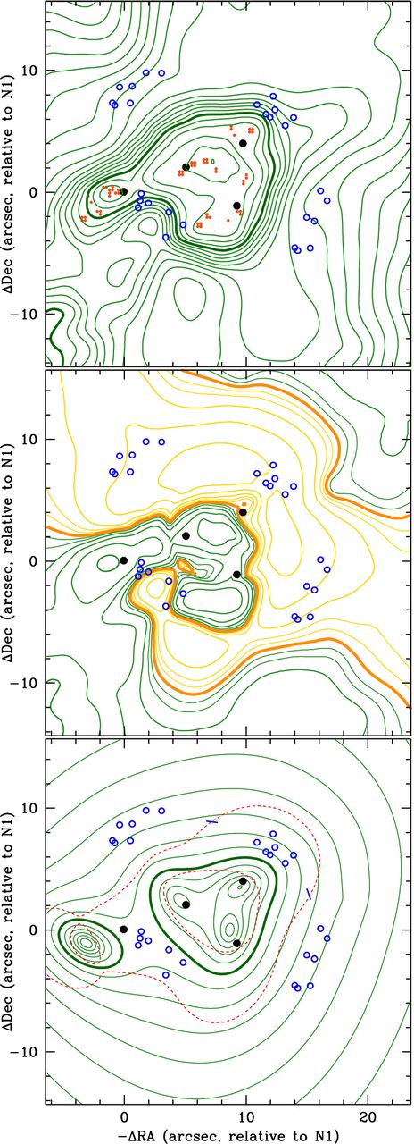
Alternative configuration L represents a minor perturbation of the strong lens image assignments, with Aa.6 switched to a fifth image of star formation knot Ab.5. In the fiducial configuration, grale reproduces the three images of knot Aa, but merged into a continuous arc, which is not consistent with their appearance on HST images. In configuration L, grale finds a mass 4.44 × 10¹² M⊙ within 10 arcsec of the peak (see Fig. B2), which is better able to reproduce the observed distribution of luminous sources near N.1. However, it introduces an extra mass clump ∼6 arcsec south of N.1 that has no identifiable optical counterpart (see Fig. B3). With this configuration, lenstool produces inconsistent predictions of the multiplicity of knot a, and an overall fit marginally worse than the fiducial model. In the best-fitting model, the total mass is 4.48 × 10¹² M⊙ within the same aperture as above. The positions of the mass peaks move only within statistical errors compared to the fiducial model (see Table B2), for this and similar minor perturbations to the image assignments.
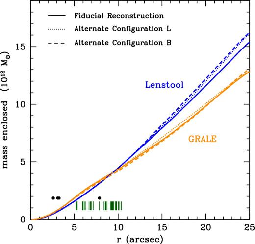
Total mass profile of the cluster core as a function of projected distance from the peak of the grale mass map, for the fiducial model versus the alternate configurations of lensed image associations. Circles along the bottom show the radial positions of cluster member galaxies N.1–4, and vertical lines mark the positions of lensed images.
Map of total mass in the cluster core, as in Fig. 4 but using alternate configuration L to associate lensed images.
Alternative configuration B had been our preferred configuration before we obtained any VLT integrated field spectroscopy. If star formation knots Aa.4–6, Ab.4 and Ac.4 are left unassigned, and the fit is optimized without any constraints in that region, the best-fitting model converges to an assignment like that in Table B1, reflecting a morphology illustrated in Fig. B1. The images immediately south of N.1 in the broad-band images are unaccounted for as strong lens sources, but point sources are frequent in this region, so they could be a chance superposition. Using these assignments, grale finds a total mass 6.06 × 10¹² M⊙ within 10 arcsec of the peak. The mass near N.1 becomes a ‘tail’ extending to the south-east (see Fig. B4). This is particularly interesting because in some models of particle physics (Kahlhoefer et al. 2014), non-zero self-interaction cross-section would indeed disperse the dark matter, rather than simply offsetting it from the light. A similar extension would also probably be expected in the case of dynamical fraction. Using configuration B, the best-fitting lenstool model with mass 4.48 × 10¹² M⊙ is apparently better than the fiducial model, with 〈rmsi〉 = 0.23 arcsec.
Map of total mass in the cluster core, as in Fig. 4 but using alternate configuration B to associate lensed images.
Changes to the assignments of multiply imaged systems in Table 2, to produce alternative configuration B. Columns denote the ID and position of the image, its major and minor axis, and the angle of the major axis on the sky, anticlockwise from west.
| Name | RA | Dec | Major | Minor | Angle |
|---|---|---|---|---|---|
| (arcsec) | (arcsec) | ||||
| Aa.4 | 330.474 47 | −59.946 180 | 0.13 | 0.09 | 90° |
| Aa.5 | – | – | – | – | – |
| Aa.6 | – | – | – | – | – |
| Ab.4 | 330.474 52 | −59.946 347 | 0.10 | 0.07 | 90° |
| Ac.4 | 330.474 40 | −59.946 032 | 0.07 | 0.06 | 70° |
Parameters of the best-fitting mass model constructed by lenstool, using alternative associations between lensed images. Positions are relative to the peak of light emission, except for the cluster-scale halo, whose position is relative to the peak of emission from galaxy N.1. Errors show 68 per cent statistical confidence limits due to uncertainty in the lensed image positions.
| σv (km s−1) | x (arcsec) | y (arcsec ) | e | θ (°) | rcore (arcsec) | 〈rmsi〉 (arcsec) | χ2/dof | log10(E) | |
|---|---|---|---|---|---|---|---|---|---|
| Alternative configuration L: | 0.26 | 50.8/23 | −27.8 | ||||||
| N.1 | 185|$^{+10}_{-11}$| | −0.43|$^{+0.17}_{-0.16}$| | −0.69|$^{+0.18}_{-0.19}$| | 0.34|$^{+0.10}_{-0.14}$| | 50|$^{+56}_{-13}$| | [→0] | |||
| N.2 | 187|$^{+42}_{-17}$| | −0.86|$^{+0.47}_{-0.33}$| | −0.40|$^{+0.30}_{-0.22}$| | 0.44|$^{+0.09}_{-0.13}$| | 176|$^{+138}_{-4}$| | [→0] | |||
| N.3 | 241|$^{+14}_{-19}$| | −0.01|$^{+0.36}_{-0.25}$| | −0.23|$^{+0.28}_{-0.30}$| | 0.35|$^{+0.07}_{-0.11}$| | 28|$^{+12}_{-12}$| | [→0] | |||
| N.4 | 261|$^{+25}_{-19}$| | −1.39|$^{+0.64}_{-0.21}$| | 0.20|$^{+0.38}_{-0.30}$| | 0.13|$^{+0.11}_{-0.13}$| | 91|$^{+57}_{-14}$| | [→0] | |||
| N.6 | 21|$^{+31}_{-11}$| | [0] | [0] | [0] | [0] | [→0] | |||
| Cluster | 711|$^{+79}_{-85}$| | 2.97|$^{+1.91}_{-0.90}$| | 1.50|$^{+1.45}_{-1.04}$| | 0.58|$^{+0.08}_{-0.14}$| | 70|$^{+6}_{-3}$| | 34.52|$^{+4.11}_{-4.17}$| | |||
| Alternative configuration B: | 0.23 | 34.5/19 | −21.3 | ||||||
| N.1 | 252|$^{+19}_{-19}$| | −3.14|$^{+0.86}_{-0.78}$| | −1.17|$^{+0.43}_{-0.40}$| | 0.43|$^{+0.08}_{-0.17}$| | 150|$^{+98}_{-17}$| | [→0] | |||
| N.2 | 216|$^{+20}_{-18}$| | −0.65|$^{+0.24}_{-0.40}$| | 0.44|$^{+0.40}_{-0.37}$| | 0.40|$^{+0.13}_{-0.10}$| | 133|$^{+18}_{-12}$| | [→0] | |||
| N.3 | 236|$^{+14}_{-26}$| | −0.15|$^{+0.34}_{-0.28}$| | −0.44|$^{+0.32}_{-0.34}$| | 0.43|$^{+0.02}_{-0.09}$| | 24|$^{+12}_{-9}$| | [→0] | |||
| N.4 | 252|$^{+16}_{-21}$| | −0.63|$^{+0.32}_{-0.29}$| | 0.97|$^{+0.36}_{-0.42}$| | 0.38|$^{+0.08}_{-0.10}$| | 80|$^{+15}_{-35}$| | [→0] | |||
| N.6 | 34|$^{+54}_{-4}$| | [0] | [0] | [0] | [0] | [→0] | |||
| Cluster | 687|$^{+63}_{-94}$| | 7.66|$^{+1.94}_{-0.81}$| | 2.66|$^{+2.12}_{-1.70}$| | 0.70|$^{+0.18}_{-0.09}$| | 69|$^{+4}_{-7}$| | 38.89|$^{+4.41}_{-5.01}$| |
Most notably, configuration B's |$3.35^{+0.74}_{-0.82}\,{\rm arcsec}$| offset between the mass and light of N.1 reproduces the result of Williams & Saha (2011). This recovery of the ground-based results is reassuring: the star formation knots near N.1 were not resolved in the ground-based imaging. However, our IFU data show this image configuration to be incorrect. [O ii] line emission is observed immediately south of N.1 in Fig. 3, inconsistent with the configuration B morphology illustrated in Fig. B1. Note that the observed line emission flux has a large spatial gradient, and is detectable even through the obscuration of N.1 because (according to our fiducial model) the gravitational lensing magnification is 53 per cent greater at the position of knot Aa.4 than at the position of knot Ad.4. The change in conclusion from Williams & Saha (2011) to this work thus emerges equally from both our new high-resolution HST imaging plus our new VLT integrated field spectroscopy, and demonstrates the discriminatory power of the combined observations.
