


Abstract
Past calibrations of statistical distance scales for planetary nebulae have been problematic, especially with regard to ‘short’ versus ‘long’ scales. Reconsidering the calibration process naturally involves examining the precision and especially the systematic errors of various distance methods. Here, we present a different calibration strategy, new for planetaries, that is anchored by precise trigonometric parallaxes for 16 central stars published by Harris et al. of USNO, with four improved by Benedict et al. using the Hubble Space Telescope. We show how an internally consistent system of distances might be constructed by testing other methods against those and each other. In such a way, systematic errors can be minimized. Several of the older statistical scales have systematic errors that can account for the short–long dichotomy. In addition to scale-factor errors, all show signs of radius dependence, i.e. the distance ratio [scale/true] is some function of nebular radius. These systematic errors were introduced by choices of data sets for calibration, by the methodologies used, and by assumptions made about nebular evolution. The statistical scale of Frew and collaborators is largely free of these errors, although there may be a radius dependence for the largest objects. One set of spectroscopic parallaxes was found to be consistent with the trigonometric ones while another set underestimates distance consistently by a factor of 2, probably because of a calibration difference. ‘Gravity’ distances seem to be overestimated for nearby objects but may be underestimated for distant objects, i.e. distance dependent. Angular expansion distances appear to be suitable for calibration after correction for astrophysical effects. We find extinction distances to be often unreliable individually though sometimes approximately correct overall (total sample). Comparison of the Hipparcos parallaxes for large planetaries with our ‘best estimate’ distances confirms that those parallaxes are overestimated by a factor 2.5, as suggested by Harris et al.'s result for PHL 932. Assuming the problem arises from the presence of nebulosity, we suggest a possible connection with the much smaller overestimation recently shown for the Hipparcos Pleiades parallaxes by Melis et al.
1 INTRODUCTION
1.1 Brief history of calibration of statistical distances
By the mid-twentieth century, when accurate distances could not generally be obtained for planetary nebulae with the usual methods (e.g. trigonometric and spectroscopic parallax), recourse was to methods based on uniformity assumptions about the physical properties of the nebulae. The hope with these ‘statistical’ methods was that the individual objects’ properties do not greatly deviate from the assumed universal value. One was the Shklovsky (1956) method, based on the assumption of identical ionized mass Mi for all planetaries; it used recombination-line theory to obtain a relation between Hβ surface brightness Sβ (presumably distance independent except for extinction) and radius R to be used with the angular diameter φ in estimating distance. Shklovsky showed mathematically that the distance estimate so obtained is fairly insensitive to the value of Mi.
Later, the Shklovsky method was modified and refined, as for example with postulated universal relations between Mi (no longer assumed constant; cf. Maciel & Pottasch 1980; Pottasch 1980) and R or between 5 GHz brightness temperature Tb (presumably unaffected by extinction, unlike Sβ) and R (cf. Daub 1982). Yet calibration remained difficult because of a dearth of accurate individual distance estimates. For a long time, one had only a small collection of miscellaneous data, some of dubious quality and hardly any of high precision, to use for calibration. In addition to the inaccuracies inherent in each kind, there can be systematic errors differing from one kind to another or even from one data set to another for the same kind.
Because of the past scarcity of high-quality data, the practice in calibrating statistical scales has usually been to follow one of two strategies: the inclusive strategy, where one simply includes all (or almost all) the various kinds of data in the calibration set, or the eclectic strategy, choosing only the ‘best’ determinations for the calibration set. With the former strategy, one hopes that the various errors, random and systematic, will average out. In fact, the result is likely a substantially larger uncertainty than the formal errors lead one to expect, and there may be some residual systematic error also. The latter strategy is likewise potentially vulnerable to systematic error; indeed, the narrower is the selection, the less likely that systematic errors will cancel out. Historically, then, different choices of data, differences in weights given to the various data and different calibration methods have produced a sizeable range of calibrations for these scales, just as one would expect when there are systematic errors.
Broadly speaking, statistical scales have divided into ‘short’ and ‘long,’ the two groups typically differing by a factor of the order of 2 (cf. e.g. Phillips 2002, hereafter Ph02). An example of the former is the scale of Cahn, Kaler & Stanghellini (1992, hereafter CKS); the latter is exemplified by Zhang's (1995, hereafter Z95) scale. This dichotomy can actually be traced back at least as far as O'Dell (1962; hereafter O62) for the ‘short’ scale and Seaton (1966; hereafter S66) for the ‘long’ one.
During the past few decades, more and better data have become available. For example, already in estimating the local space density of planetaries Pottasch (1996, hereafter P96) made use of (among others) eight spectroscopic parallaxes of companions of central stars, six distance estimates from angular expansion rates, and 30 from extinction (either line or continuum) as a function of Distance. Ciardullo et al. (1999, hereafter C99) used the Hubble Space Telescope (HST) to search for more central star companions, considerably augmenting the number of spectroscopic parallaxes. The angular expansion method, originally applied to optical images, has been extended to radio images with the VLA (Terzian 1980; Masson 1986; cf. esp. Terzian 1997); the optical version has been improved with the replacement of photographic plates by CCD's and the use of HST (e.g. Reed et al. 1999; Palen et al. 2002). An astrophysical method based on fitting central star spectral line profiles to those from stellar atmosphere models and matching the properties to evolutionary tracks has been developed (Méndez et al. 1988) yielding what are termed ‘gravity’ distances (referring to surface gravity) that can be used for calibration. Lastly, new techniques have been applied to measuring central stars’ trigonometric parallaxes, finally bringing those within reach. Parallaxes have been obtained using the Hipparcos satellite (Acker et al. 1998, hereafter A98), the HST fine guidance sensors (Benedict et al. 2003), and ground-based CCD cameras (Pier et al. 1993; Harris et al. 1997, hereafter H97; and Gutiérrez-Moreno et al. 1999).
The trigonometric parallax method has the virtues that it is geometrical and thus direct and, in principle at least, is model independent; at least, it involves no astrophysical assumptions or modelling. The parallax should be valid for the nebula provided that the central star is correctly identified and, if needed, the correction for the reference stars’ parallaxes (i.e. relative to absolute) is done properly. There is also no need to correct for interstellar extinction. While the method's applicability is necessarily limited at present to nearby planetaries, it can be used to evaluate and/or calibrate other methods of greater reach. In the near future, the range is expected to be greatly extended because of the Gaia observatory (Perryman et al. 2001; Manteiga et al. 2012; Manteiga et al. 2014).
Unfortunately, five of the 19 original Hipparcos central star parallaxes in A98 were negative, while the remainder were not very precise, with a median relative parallax error |$\lambda \equiv \sigma _\pi ^\prime /\pi ^\prime$| of 0.66. (Here, as usual π′ is the measured parallax and |$\sigma _\pi ^\prime$| is the estimated standard error of the parallax; the corresponding true values are π and σπ, respectively) The median λ for the three obtained by Gutiérrez-Moreno et al. was almost the same, 0.69, while the H97 ones were much better, with median λ of 0.34, but on the whole still not highly precise. The HST fine guidance sensors are capable of very high precision but until recently had yielded only one parallax measurement for a planetary.
While some of the notation we use is standard, much – e.g. the use of λ for relative parallax error – is not and likely is unfamiliar to the reader. At the end, there is an appendix with a list containing definitions and first locations in the text.
1.2 Accurate parallaxes and the ‘anchor’ strategy for calibration
In the past several years, the situation has improved considerably. An expanded sample (N = 16) of high-quality CCD parallaxes was published by the USNO group (Harris et al. 2007, hereafter H07). These parallaxes have a median error of 0.42 mas and a median λ of 0.17, an improvement of a factor of 2 over their previous work. More recently, four of these objects were studied using HST (Benedict et al. 2009, hereafter B09). The precision of those measurements is even greater, with median error 0.23 mas and median λ = 0.08. The results of the two studies are in generally good agreement: The median parallax ratio H07/B09 is 1.17 and the mean is 1.19 ± 0.09, indicating that there might be a slight systematic difference between the two. We will discuss this question in the next section, arguing that there is in fact no significant systematic difference.
We believe that accurate trigonometric parallaxes can serve as a solid foundation on which to erect an interlocking structure of distance determinations from various methods. This idea is not new; of necessity that is largely what happened with stellar distances, and in O62 O'Dell lamented the absence of astrometric data to fill precisely this role with planetaries. For a long time, the inclusive and eclectic strategies appeared to be the only choices. We contend that space observatories and CCD cameras have changed that.
In this paper, we demonstrate what we term the ‘anchor’ strategy for calibration. Our calibration is anchored by the parallaxes, which serve to check other methods which can be used to verify still others, and so forth. For our strategy to succeed, it is essential that no appreciable systematic errors be present in the parallax data or be introduced by our methodology. We then take pains to eliminate or mitigate any systematic errors in the other data types by comparing those with the parallax data, either directly or, if need be, indirectly and applying corrections or modifying our techniques.
In order to be able to track down systematic error, it is highly desirable to have large, reasonably homogeneous data sets. If instead one has merely a hodgepodge of meagre data from different sources, using different instruments and/or reduction methods, it can be difficult to tease out any systematic differences. As an extreme example, with only one parallax obtained from HST (as was the case in 2007), one could not really compare that approach with the CCD one.
For convenience, the parallaxes for the USNO sample are presented in Table 1 along with corresponding angular diameters φ and R values. Parallax values are from H07 except for the ones marked with asterisks, which are weighted means of the H07 and B09 values taken from the latter source. Angular diameters are mostly optical values taken from the Strasbourg-ESO Catalogue (Acker et al. 1992, hereafter A92). For NGC 7293, we have used the radio value rather than the optical one in order to leave out the faint outer halo; it is almost identical to the optical value 654 arcsec given in O'Dell (1998). We likewise have ignored the very faint extended halo found for PG 1034+001 (Rauch, Kerber & Pauli 2004) and instead used the original value from Hewett et al. (2003). The values for RE 1738+665 and Ton 320 are from Tweedy & Kwitter (1996), while the value for Sh 2-216 is from Tweedy, Martos & Noriega-Crespo (1995). Our φ values are in most cases fairly close to those used with the statistical scales we consider; correcting for obvious errors the mean ratio of those to ours is 1.00 ± 0.11 (s.d.) for CKS and 0.96 ± 0.07 (s.d.) for Z95. For the mean statistical scale of Frew (2008; hereafter F08) the mean is 1.07 ± 0.03 and the median 1.04, indicating ours are slightly smaller.
Observational data and radii for the USNO trigonometric parallax sample of H07.
| Name | π′ (mas) | φ (arcsec) | R (pc) |
|---|---|---|---|
| A 7 | 1.48 ± 0.42 | 760 | 1.25 |
| A 21 | 1.85 ± 0.51 | 615 | 0.81 |
| A 24 | 1.92 ± 0.34 | 355 | 0.45 |
| A 31 | 1.61 ± 0.21* | 970 | 1.46 |
| A 74 | 1.33 ± 0.63 | 830 | 1.51 |
| DeHt 5 | 2.90 ± 0.15* | 530 | 0.44 |
| HDW 4 | 4.78 ± 0.40 | 104 | 0.053 |
| NGC 6720 | 1.42 ± 0.55 | 76 | 0.13 |
| NGC 6853 | 2.47 ± 0.16* | 402 | 0.32 |
| NGC 7293 | 4.66 ± 0.27* | 660 | 0.34 |
| PG 1034+001 | 4.75 ± 0.53 | 7200 | 3.68 |
| PHL 932 | 3.36 ± 0.62 | 275 | 0.20 |
| PuWe 1 | 2.74 ± 0.31 | 1200 | 1.06 |
| RE 1738+665 | 5.91 ± 0.42 | 3600 | 1.47 |
| Sh 2-216 | 7.76 ± 0.33 | 5840 | 1.83 |
| Ton 320 | 1.88 ± 0.33 | 1800 | 2.32 |
We present evidence below that the H07 parallaxes themselves are with one exception free of systematic error such as might arise from the use of two different CCD cameras and are otherwise consistent with the B09 parallaxes. Of course systematic error can be introduced by the methodology employed when using parallaxes, e.g. Lutz–Kelker-type bias; that and others will be considered in Section 2.
Two important limitations of the H07 sample are evident in Table 1. First, no object is likely to be more distant than 1 kpc. Hence, the H07 sample by itself is unsuited to exploring distance dependence, i.e. the distance ratio [scale/true] depending upon distance. Secondly, most of them are fairly large. This is to be expected, for planetaries with low surface brightness S should cause relatively little interference with position measurements of the (often faint) central stars, and large R goes with low S. Indeed, there were obviously problems with the Hipparcos measurements for planetaries having small angular sizes and high surface brightnesses, as noted in A98. There is only one H07 object smaller in R than 0.1 pc, and it may not be a planetary nebula, as discussed below. There is a preponderance of objects with low Tb at 5 GHz as well, the sample values (shown below) almost all less than 1 K. For this reason, the H07 sample is of limited usefulness by itself in assessing any systematic error depending on R or Tb. We show below an example of a distance dependence, and radius dependence (distance ratio depending on nebular radius) is common.
The calibration of a statistical scale built upon a Tb–R or S–R relation involves estimation of at minimum two parameters, a zero-point and (for log–log relations) a slope, and in principle the slope may vary with R. Extrapolating the slope found with the H07 sample to smaller R risks introducing a radius dependence into the scale if the true slope differs. On the other hand, use of a different sample such as a set of spectroscopic parallaxes to fix the relation at smaller R injects the problem of heterogeneity with its potential for systematic error, for example with a calibration for the spectroscopic parallaxes that is inconsistent with the trigonometric ones (an example to be provided below).
We can use the H07 sample to indirectly evaluate other methods by means of an intermediary distance scale. If the method to be evaluated can be assumed to have no radius or distance dependence (e.g. with spectroscopic parallax) and if each sample has a substantial presence within a given limited range in R that method's relative precision and error in zero-point can be estimated. In this way, it might be possible to establish an internally consistent calibration over a wider range in R and estimate the variation in slope within that range, if any. The process can then be repeated to further extend the range. What we are outlining is the stepwise construction of an interlocking system of distance determinations.
1.3 Classification complications arising with calibration
Another problem, similar to the one with combining distance estimates from different methods, is that there is copious evidence that the objects called planetary nebulae do not comprise a homogeneous class. To be sure, there are some objects that have been misclassified as planetaries (cf. e.g. Acker & Stenholm 1990), and this seems to be true of a few objects in the H07 sample, as noted directly below. However, apart from such cases there appear to be differences among the nebulae in chemical composition, kinematic properties and spatial distribution (Peimbert 1978) which are interpreted as being due to differing progenitor masses (cf. e.g. the discussion in Quireza, Rocha-Pinto & Maciel 2007). Unfortunately, only a relatively small fraction of known planetaries have been classified, and among the objects we consider here fewer than half have been, so we cannot pursue that thread in this paper given our modest sample sizes.
Frew & Parker (2006) identified five objects in the H07 sample – RE 1738+665, DeHt 5, PHL 932, HDW 4, and PG 1034+001 – as possibly being associated with ionized interstellar medium (ISM) rather than being true planetary nebulae. These identifications are supported by Frew & Parker (2010) and specifically for PHL 932 by Frew et al. (2010) and for PG 1034+001 by Chu et al. (2004). A 35 was classified as an H ii region in F08; it is not a member of the H07 sample but will be considered in connection with the Hipparcos parallaxes in Section 6. We provisionally accept the classification of these (following F08) as ‘imposters.’
In the next section, we address the bias issue for trigonometric parallaxes, both for the overall distance scale of the H07 sample and for a possible sample-dependent bias of individual parallaxes caused by the Lutz–Kelker effect. We also consider the bias in overall distance ratio arising with sample selection based on statistical distances and biases with several estimators used when comparing distance scales. In Section 3, we use H07 parallaxes to test our representative examples of the ‘short’ and ‘long’ statistical scales, respectively, CKS and Z95, along with the mean F08 scale. We check the C99 spectroscopic parallaxes against H07 indirectly, using the statistical scales, with nebulae in the range of overlap, namely −1 < log R < 0; then, we use both the H07 and C99 data sets to cover a fairly wide range in R in our testing of the statistical scales. We examine the Tb–R relation generally in Section 4, adding data on Magellanic Cloud planetaries to extend the range in R even further, and briefly relate the relation to evolution of the star+nebula systems. The gravity, angular expansion and interstellar extinction distances are tested in Section 5. In Section 6, we consider the Hipparcos trigonometric parallaxes, which we have not used in this paper for testing or calibration, comparing them to our ‘best estimates’ and demonstrate their systematic error for large objects. We propose an explanation of the long-standing dichotomy in statistical distance scales in the context of calibration strategies in Section 7. Our conclusions are summarized and discussed in the final section, where we make a few suggestions for future work.
2 THE BIAS PROBLEM WITH TRIGONOMETRIC PARALLAXES
2.1 Some general considerations
When earlier trigonometric parallax data suggested the gravity distances were overestimated, Napiwotzki (2001, hereafter N01) pointed out that the cause might instead be Lutz–Kelker bias. He carried out Monte Carlo simulations using a fairly realistic model of the spatial distribution of planetaries and found an underestimation of approximately the right amount. Strictly speaking, the bias he found was of the Trumpler–Weaver type (Trumpler & Weaver 1953), since he imposed a lower limit on the measured parallaxes in his synthetic samples. Nevertheless, some similar bias might affect a distance scale comparison in the absence of a lower limit. In N01, the bias was evaluated numerically because the classical Lutz–Kelker corrections, originally devised to counter Trumpler–Weaver bias, assumed a uniform spatial distribution, whereas N01's model was more complicated.
Trumpler–Weaver bias is an example of truncation bias, which can arise when selecting a sample based on a limited range of values of quantities that have errors of measurement. The original idea was that when a sample of parallaxes is truncated at some lower limit |$\pi ^\prime _{\rm l}$| the remaining parallaxes will have an excess of positive errors as well as a deficiency of negative errors and hence a positive bias. The discarded parallaxes will include some with true parallax |$\pi >\pi ^\prime _{\rm l}$| (negative error), while some parallaxes with |$\pi <\pi ^\prime _{\rm l}$| (positive error) will be erroneously included. Sometimes, the sample is truncated according to λ instead of π′, with an upper limit instead of a lower limit; again, the result is a positive bias (Arenou & Luri 1999; Pont 1999). Obviously, if one wishes to avoid truncation bias, the best way is to include all parallaxes regardless of relative error, or sign for that matter – in other words, no truncation.
Another kind of bias that can arise is transformation bias, as when one converts measured parallaxes with their errors into distances or magnitudes (cf. e.g. Smith & Eichhorn 1996, hereafter SE96; Brown et al. 1997). N01 noted that the conversion of parallaxes to distances is problematic when comparing distance scales, for this very reason. The problem can be avoided by not converting the parallax; indeed, working strictly in the parallax space has already been suggested (e.g. Arenou & Luri 1999).
On the other hand, if instead of multiplying the distance estimate by the parallax one computes the distance from the parallax and then divides by the comparison distance, as was done in A98, the expectation of the result will in general not equal the reciprocal of the true distance ratio. The mean of the distances computed from the measured parallaxes (including errors) for a given object does not equal the true distance, as was shown in SE96, and the mean of the reciprocals of the distance estimates being compared will also be biased (transformation bias). Therefore, the mean of the product of the two will in general be biased as well.
This weighting bias was explored with a set of idealized Monte Carlo simulations. Three different distance distributions were used: (1) uniform density in 3D (spherical), (2) uniform density in 2D (disc) and (3) uniform density in 1D (flat). All three were sampled to a maximum distance dmax, which was varied to evaluate its influence on the amount of bias. To simulate the statistical distance estimation method, the randomly chosen true distance d of each object was multiplied by the scale factor B chosen for that run (value 0.7, 2, or 4) to give dS; then a random error was added sampled from a Gaussian having standard deviation σd = αSdS where αS is a measure of the relative distance error for that scale (chosen as 0.35, 0.4, or 0.45 for each run) to give a pseudo-distance; the Gaussian was truncated at ±2σd. The true distance was also converted into a parallax and an error added selected at random from a Gaussian whose standard deviation was itself randomly chosen over a variable range, from 0.3 to as much as 1.3 mas.
A fairly representative set of results of simulations for 10 samples of N = 1000 stars each are shown in Table 2. The spatial distribution used for these was the disc distribution, B was 2, the spread of the parallax errors was roughly from 0.3 to 0.5 mas and α was 0.4. As expected, the unweighted mean distance ratio obtained by multiplying the pseudo-distances by the parallaxes generally gave the correct value for B to within the uncertainty. On the other hand, the negative weighting bias showed up quite clearly in the weighted mean ratios. The amount of bias depends on the limiting distance because of the first and third terms on the rhs in equation (1a). It becomes of the order of −15 per cent when the limiting distance approaches 1 kpc.
Unweighted and weighted mean and Phillips κ as estimators of distance ratio based on parallaxes, using synthetic data with B = 2 and a disc distribution.
| dmax (pc) | Unweighted | Weighted | κ |
|---|---|---|---|
| 200 | 2.005 ± 0.008 | 1.969 ± 0.008 | 1.996 ± 0.009 |
| 500 | 1.982 ± 0.006 | 1.827 ± 0.007 | 1.907 ± 0.013 |
| 700 | 1.995 ± 0.008 | 1.742 ± 0.009 | 1.751 ± 0.032 |
| 1000 | 2.001 ± 0.012 | 1.642 ± 0.012 | 1.903 ± 0.510 |
| 1500 | 2.003 ± 0.015 | 1.521 ± 0.012 | 1.554 ± 0.246 |
Having said this, we must point out that κ is actually a very good measure of the mean distance ratio if one uses distances in the denominator which are not derived from parallaxes but instead have something like a normal error distribution. Table 3 gives a typical set of results for the same spatial distribution and B as in Table 2 but for distances |$d^\prime _1$| not derived from parallaxes, ones which have relative errors α1 = 0.40 (roughly comparable to the typical λ for the parallaxes in the previous case) and the same relative error α2 for the second scale. We have not assigned weights to the values because the relative errors are all the same. Obviously, the average of the individual distance ratios is biased, whereas κ is not. The bias of the former is formally equivalent to the bias pointed out in SE96 for the mean of the distances obtained from parallaxes; fig. 1 of that paper suggests that for α = 0.4 there should be a positive bias of roughly 20 per cent, while the actual figure is 18 per cent. (The difference might largely be due to the 2σ truncation of the Gaussian in our experiments.) Indeed, we should expect κ to be asymptotically unbiased, since the errors in both numerator and denominator are presumably symmetric when there is no truncation of the sample according to d′, as in this case, and therefore positive and negative errors should tend to cancel out in both places. Incidentally, the same would be expected for the ratio of sums of parallaxes. Additionally, we see in these experiments that κ seems to have a smaller uncertainty than does the mean distance ratio. These conclusions are supported by a more extensive set of numerical experiments which we will not present here. Finally, for a given set of objects κ is strictly transitive, i.e. for three distance scales A, B and C the overall distance ratio A/C equals the ratio A/B times the ratio B/C, a nice property not shared with many other estimators.
Unweighted mean, Phillips κ, and ζ (see text) as estimators of distance ratio comparing two statistical distance scales, using synthetic data with B = 2 and a disc distribution.
| dmax (pc) | Unweighted | κ | ζ |
|---|---|---|---|
| 200 | 2.381 ± 0.021 | 2.008 ± 0.013 | 1.900 ± 0.011 |
| 500 | 2.362 ± 0.011 | 1.998 ± 0.010 | 1.892 ± 0.007 |
| 700 | 2.355 ± 0.018 | 1.971 ± 0.014 | 1.913 ± 0.011 |
| 1000 | 2.375 ± 0.018 | 2.006 ± 0.011 | 1.904 ± 0.012 |
| 1500 | 2.336 ± 0.016 | 1.984 ± 0.008 | 1.914 ± 0.010 |
There are two important reservations concerning κ, however. First, if the sample does not have a smooth distance distribution like the synthetic samples just considered but instead has one object with a distance that is much greater than those of the rest, its distance ratio will dominate the result. For example, there is a planetary nebula in the globular cluster M 15 whose distance is at least an order of magnitude greater than the typical distances of planetaries in the local solar neighbourhood. More generally, κ gives higher weight to more distant objects. As a result, if there is a distance-dependent systematic error in the distance ratio, κ will tend to reflect the value appropriate to the most distant members of the sample. Hence, there needs to be a modification to more nearly balance the contributions to the estimator from objects with widely differing distances. Below, we propose a weighting scheme intended to do precisely that. Secondly, κ is only a metric for comparing distance scales on average, not assessing how exactly individual distances in one scale follow those in another. The oft-used Pearson correlation coefficient r is conventionally chosen for the latter purpose. By its form, however, it ignores any scale factor difference that might be present. It, too, suffers from a sensitivity to isolated extreme values.
Individual values of log R are of interest in connection with both any possible radius dependence of distance ratios and their relation to log Tb or log S. Estimates of log R based on parallaxes are affected by transformation bias (through the log function acting on distance d′) together with a double truncation bias, a combination sometimes mistakenly thought of as universal for absolute magnitudes M: Lutz–Kelker bias (Lutz & Kelker 1973). As the author pointed out (Smith 2003), the effect of the combination is not intrinsic and universal as originally claimed but rather depends on the characteristics of the particular sample; this fact is clearly demonstrated by figs 3 and 4 of that paper. Especially in fig. 4 one sees that the mean of the error in absolute magnitude ΔM caused by distance error, which in fact is proportional to the error in log R for nebulae, is a function of λ not necessarily given by the negative of the classical Lutz–Kelker corrections. Indeed, it is not necessary that there be any Trumpler–Weaver bias for the sample in order for this Lutz–Kelker effect to act on individual values, even though that bias is what the corrections were originally intended to cancel out. Whereas the sample shown in fig. 4 is formally truncated at λ = 0.175, it is effectively limited by the apparent magnitude cut-off at ml = 7; therefore there is no truncation bias for the parallax sample as a whole.
In evaluating the individual bias as a function of λ in the particular case, we started with the (assumed) distribution of true parallaxes g(π) and added errors ϵπ selected randomly from a normal distribution with the value of σπ assumed to be the same for all stars independent of π. Computing the bias is then straightforward. In the real world, of course, the situation is quite different: one often does not know g(π) or at best only approximately; almost certainly σπ will have a distribution which is different for each value of π; and one has only an estimate of σπ, namely |$\sigma _\pi ^\prime$|, when forming the ratio λ. This last is probably a relatively minor problem; seemingly it should result in nothing more than a ‘smearing’ of the distribution compared to the true one. On the other hand, variations in the distribution of σπ and thus that of ϵπ with π introduce a higher degree of complexity.
The inversion problem, namely going from the (normalized) observed distribution |$\phi (\pi ^\prime ,\sigma _\pi ^\prime )$| to the underlying distribution Φ(π, σπ), formally seems rather difficult. Instead, we will merely try to find a model Φ which gives a fairly decent match to the observed ϕ, keeping in mind that there are probably some other such functions Φ that will give a fit that is as good or possibly even a little better. For our present purposes, it is likely unnecessary to obtain an optimum fit to ϕ, however. For the H07 sample, we will attempt to use the selection criteria (insofar as they can be inferred) together with some other information to constrain the model.
2.2 Bias with the H07 parallax sample
To the best of the author's knowledge, the exact criteria used in choosing the actual H07 sample have never been published. The nearest approaches to a specific statement on this subject are a comment at the end of H97 about adding nebulae that ‘are likely to be at a distance closer than 500 pc’ and the information on the model used to show that the bias is small which appears near the end of H07 (see next paragraph). There is no explicit truncation on the basis of either π′ or λ, so one would expect no Trumpler–Weaver bias. To be sure, there was one planetary, A 29, which was dropped from the USNO programme list because its astrometric solution was not stable, but the provisional value published in H97, 2.18 ± 1.30 mas, was not negative or unusually small. We believe that the faintness of its central star, V = 18.31, rendered it unsuitable for parallax measurement.
The model used in H07 when considering possible bias was based on an underlying spatial distribution of planetaries similar to that of N01, namely an exponential z-distribution with a scaleheight z0 of 250 pc and selection according to statistical distance with upper limit 550 pc for a distance scale having αS = 0.3 and B = 1. Their model apparently gives a fairly good fit to the marginal distributions of π′, |$\sigma _\pi ^\prime$|, etc. as indicated by the first and second moments.
However, such a model has a potential problem when one evaluates overall distance ratios for statistical distance scales. Truncation of the sample on the basis of statistical distance (not parallax) might well introduce a bias in the distance ratio because of an excess of negative distance errors together with a deficit of positive errors. This bias could arise to some extent even if the statistical scale used for selection is different from the one being tested, if both are based on essentially the same approach and use the same or related data (such as Hβ or photored flux and 5 GHz flux density). We emphasize that this problem has nothing to do with any bias of the trigonometric parallaxes themselves.
To assess this effect, we have looked into the selection of the H07 sample as related in the USNO group's papers (Pier et al. 1993; H97; H07). Briefly, half of the H07 sample objects appear to have been selected because they were on the list of nearby planetary nebulae compiled by Terzian (1993, hereafter T93) with distances smaller than 300 pc largely based on combinations of estimates from five variants of the Shklovsky method. We refer to this group as the T93 subsample; it is at risk of the selection bias described above. The remaining objects in the H07 sample were selected for other reasons – association with nearby white dwarfs such as Ton 320 (Tweedy & Kwitter 1994), perhaps large φ as with PG 1034+001 (Hewett et al. 2003), or possibly because it is a well-known planetary with a suitably faint central star (NGC 6720). The latter are not at risk of this bias. However, five of these – DeHt 5, HDW 4, PG 1034+001, PHL 932 and RE 1738+665 – have been classified as H ii regions (see Section 1.1) and therefore cannot be used to test statistical scales (but can be used for others). Those five are our imposters (following F08); the three others comprise our non-T93 subsample and have non-statistical distance estimates ranging up to 700 or 800 pc.
The key issue here is the degree of correlation between whatever statistical distance scale is being studied and the T93 distances that were used (in part) for sample selection. Representative examples of the ‘short’ and ‘long’ statistical scales are CKS and Z95, respectively. They are also fairly comprehensive, having two of the largest overlaps (∼50 per cent) with the H07 sample of the various scales. Fig. 1(a) shows the ratios of the CKS distance estimates to the T93 ones (for the entire overlap, not just the H07 sample). Essentially, half the ratios lie between 0.9 and 1.1, indicating a very close connection between the two scales. By contrast, the ratios of the Z95 distances to the T93 ones, shown in Fig. 1(b), are widely scattered around the mean value. Obviously, there is little correlation between the Z95 and T93 distance estimates, so there should be no significant bias in that comparison.
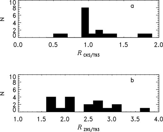
(a) Distribution of distance ratios |${\cal R}_{\rm CKS/T93}$| for nebulae common to both those lists, with the mean value being 1.1; (b) distribution of distance ratios |${\cal R}_{\rm Z95/T93}$| for nebulae in common to both those lists, with the mean value being approximately 2.5. Both values leave out the object LoTr 5, which has anomalously high values for both scales, respectively, 15.74 and 21.73, and has been omitted from both figures. (A referee pointed out that φ for this object is in error.)
To roughly estimate the effect of this bias with the CKS scale, we have generated synthetic samples of 4000 nebulae resembling the H07 model, with an underlying disc distribution having scaleheight z0 = 250 pc and selected according to a pseudo-distance limit with several different choices of B, the distance scale factor and αS. Two values of this limiting pseudo-distance were chosen, 300 and 500 pc; anticipating our later results, we used αS = 0.3, 0.35 and 0.4 and B equal to 0.7, 1.0 and 2.0. The results were found to be essentially the same for both limiting distances, namely an underestimation of B by a factor 0.70. The amount of bias depends significantly on α: if αS is 0.30, the underestimation factor is 0.79, whereas if it is 0.40 this factor is 0.59. The greater the relative spread in pseudo-distance around the true scaled value, the greater the underestimation, as would be expected.
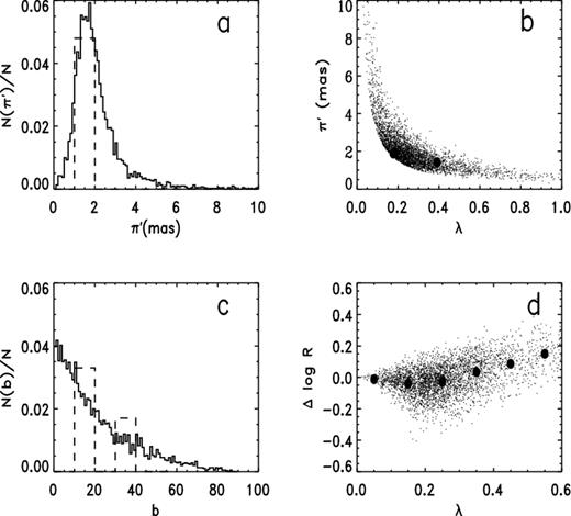
Following the reasoning laid out in the preceding paragraphs, we have generated multiple realizations of two synthetic subsamples which together model the H07 sample (with imposters removed). One subsample was selected from a model distribution very similar to that of H07 (with z0 = 250 pc) according to pseudo-distance with αS = 0.35, the limiting dS chosen as 300 pc, and B = 0.8 as above, essentially imitating the T93 sample. The other subsample was chosen from the same underlying spatial distribution purely according to limiting true distance; the value 800 pc was chosen based on the parallax distribution for the non-T93 objects. The values of σπ were chosen at random between 0.3 and 0.8 mas for both synthetic samples. Figs 2(a)–(c) show the parallax distribution, a plot of π′ versus λ and the distribution in Galactic latitude b for the T93 subsample together with corresponding plots for one realization of the model. The same plots are shown for the non-T93 objects and the second synthetic subsample in Figs 3(a)–(c). In Figs 2(b) and 3(b), the sharply defined lower envelope for the synthetic subsamples is caused by the sharp lower limit on |$\sigma _\pi ^\prime$|, which is 0.3 mas. Altogether, the model seems to give a fairly good fit to the H07 points, but of course the latter are quite sparse, especially for the non-T93 subsample. Figs 2(d) and 3(d) show the error in log R, Δ log R, resulting from the parallax errors as a function of λ for the respective synthetic subsamples, with the filled circles being the means for bins of width 0.10 in λ. (As noted above, Δ log R is proportional to ΔM that is commonly shown in such plots.) There is only a very slight underestimation of log R for small λ, whereas there is a modest overestimation at the largest values of λ. The nebulae in the H07 sample most likely to be affected by the latter are A 74 (λ = 0.47) from the T93 subsample and NGC 6720 (λ = 0.39) from the non-T93 subsample. Based on several realizations of the synthetic subsamples, we estimate that these two objects need corrections in log R of −0.10 and −0.06, respectively. These amounts are actually less than the respective errors in log R.
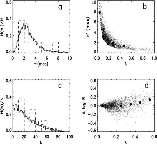
Representative properties of the T93 synthetic sample: (a) distribution of π′; dashed histogram is for H07 sample; (b) plot of π′ versus λ with the filled circles representing the H07 objects; (c) the distribution in galactic latitude b, H07 sample as in (a); and (d) the plot of Δ log R versus λ, with the filled circles now being the means for bins of width 0.1 in λ. For more details about both the synthetic samples, see the text.
Similar plots for the imposters are not shown because they cannot have trustworthy statistical distances. While we have not used them for tests of statistical distances, we have sometimes employed them in tests of other distance methods when it seemed appropriate. Simulations for them suggest the error Δ log R is negligible in all cases.
Later, we will briefly consider the effect of observational selection respecting S, which implies selection according to R. While the latter could in principle affect the form of g(π) and hence the value of Δ log R we do not consider NGC 6720 in particular to have been selected for the H07 sample in such a way. Hence, we do not see a need to modify g(π).
2.3 Estimation of typical relative errors in statistical distances using trigonometric parallaxes
Our idealized Monte Carlo experiments indicate that this approach can sometimes lead to an underestimation of αS that depends on dmax. The reason is that the term |$d_i^{\prime 2}\sigma _\pi ^{\prime 2}=(d_i+\epsilon _{d,i})^2\sigma _\pi ^{\prime 2}$| has on average an extra contribution due to the square of the error ϵd, i which increases with dmax and is subtracted from the numerator but added to the denominator. There is also an effect due to the use of π′ in place of π. As Table 4 demonstrates, this underestimation can be appreciable. When the actual values are used in place of the observed ones, the true α is approximately recovered.
Estimation of αS for 10 synthetic samples (N = 1000) with different values of dmax; αtrue = 0.36.
| dmax (pc) | |$\alpha _{{\rm S}}^\prime$| | |$\alpha _{{\rm S}}^\prime /\alpha _{{\rm S}}$| |
|---|---|---|
| 200 | 0.333 ± 0.003 | 0.925 ± 0.008 |
| 500 | 0.326 ± 0.002 | 0.906 ± 0.006 |
| 700 | 0.319 ± 0.003 | 0.886 ± 0.008 |
| 1000 | 0.312 ± 0.009 | 0.867 ± 0.025 |
| 1500 | 0.274 ± 0.006 | 0.761 ± 0.017 |
The statistics in Table 4 are for relatively large samples. With a small sample such as those considered below, equation (5) may not have a real solution. Numerical experiments for samples with N = 10, which is comparable to the typical sample sizes used here, indicate that the fraction of samples that do not yield a real solution increases with dmax and with σπ and decreases with increasing αS. For example, for αS = 0.36 and dmax = 700 pc with typical error sizes only 11 of 100 samples failed, whereas for α = 0.18 that number was 36. We infer that such failure is suggestive of small αS.
We now consider the estimated characteristics of synthetic samples which model the H07 subsamples referred to above. The CKS and Z95 scales are treated separately because we believe the sample selection distances are correlated for the former but not the latter. Five synthetic samples with N = 4000 were used for each case to evaluate the bias. If the entire T93 subsample had been selected using the CKS distances with an assumed B = 0.8 and αS = 0.35, the unweighted mean distance ratio would be 0.575 ± 0.001 and the weighted mean 0.425 ± 0.001; the weighting bias is −0.15. The reduction factor for the unweighted mean arising from the correlation in distance, 0.72, is close to the value of 0.70 found with our idealized calculations. For the same subsample but with a set of distances different from that used for selection (yet still having the same underlying spatial distribution), the corresponding values would be 0.804 ± 0.002 (no appreciable bias, as expected) and 0.511 ± 0.004 (weighting bias −0.29). The non-T93 subsample gives values 0.798 ± 0.001 (practically no bias) and 0.584 ± 0.002 (weighting bias −0.21), respectively.
In the case of Z95, we use instead the value B = 1.5 while keeping αS at 0.35. The unweighted mean for the T93 sample, once again with uncorrelated statistical distances, is 1.507 ± 0.003 and the weighted mean 1.103 ± 0.005 (weighting bias −0.40). The corresponding values for the non-T93 sample are 1.495 ± 0.001 and 1.094 ± 0.003, respectively (weighting bias the same). As will become evident later, these values ought to be fairly close for the two cases.
The estimation of αS using equation (5) is complicated; not only is there underestimation caused by the errors in distance and parallax and the numerical difficulty, but when the distances are correlated there can be overestimation instead of underestimation. With B = 0.8 and αS = 0.35 (appropriate to CKS), the T93 subsample yields |$\alpha _{\rm S}^\prime = 0.364\pm 0.001$| with correlation and 0.311 ± 0.003 without. The magnitude of these effects depends on α: for αS = 0.3 with correlation, we have 0.295 ± 0.002 (apparently the effect of the errors is virtually cancelled out by the effect of the distance correlation) and without correlation we get 0.244 ± 0.002, while when αS = 0.4 the respective values are 0.457 ± 0.006 (evidently the correlation has the upper hand) and 0.321 ± 0.002. The non-T93 subsample with αS = 0.35 yields |$\alpha _{\rm S}^\prime = 0.283\pm 0.001$| or 0.81 times the true value; the latter ratio only changes slightly when one increases or decreases the true α by 0.05, and it stays the same when one goes to B = 1.5 at αS = 0.35 (the Z95 case). The T93 subsample with B = 1.5 (for the tested distances, not those used for selection) gives a value 0.276 ± 0.003, essentially the same as for the non-T93 subsample.
2.4 Homogeneity of the H07 parallax sample
The original H07 data were obtained using two different CCD cameras, a TI800 and a Tek2048. Six objects were observed with the former, 13 with the latter and three objects with both. The ratio of the sums of parallaxes Tek2048/TI800 for the three nebulae in common is 1.08 ± 0.10. The error estimate has been obtained using the jackknife method (cf. Lupton 1993, p. 46). However, the ratio for NGC 6853 by itself is 1.45, and the difference between the two is 2σ according to H07. On the other hand, its TI800 value, 2.63 ± 0.43 mas, is not far from the value obtained with the HST FGS, while the Tek2048 value is 3.38σ away. The other two planetaries studied using both CCD cameras, Sh 2-216 and PuWe 1, have a combined ratio of 0.99 ± 0.12.
All four of the H07 nebulae studied in B09 have parallaxes obtained with the Tek2048. Excluding NGC 6853, the ratio of the sums of parallaxes for the B09 sample in the sense Tek2048/FGS is 1.08 ± 0.09. Therefore, we conclude that there is no evidence for an appreciable systematic difference among the H07 parallaxes or between the H07 and B09 parallaxes. The Tek2048 parallax for NGC 6853 appears to be anomalous. In H07, the authors suggested the cause was contamination by light from a faint companion which depended on seeing. Despite the problem we none the less incorporate it into the weighted mean, following B09.
3 COMPARISON OF STATISTICAL DISTANCE SCALES WITH PARALLAXES
3.1 The ‘short’ CKS scale
Table 5 presents the distance values from CKS and the individual distance ratios |${\cal R}_{{\rm CKS}}$| together with their uncertainties |$\sigma _{\cal R}$| according to equation (1a). The imposter PHL 932 is included in the table but omitted from our analysis. For estimating |$\sigma _{\cal R}$|, the value αCKS = 0.35 was used, obtained after correcting for the bias mentioned in Section 2.3 using the combined data from the synthetic subsamples as described below.
| Name | dCKS (pc) | |${\cal R}_{{\rm CKS}}\pm \sigma _{\cal R}$| |
|---|---|---|
| A 7 | 216 | 0.32 ± 0.15 |
| A 21 | 243 | 0.45 ± 0.20 |
| A 24 | 525 | 1.01 ± 0.40 |
| A 31 | 233 | 0.38 ± 0.14 |
| NGC 6720 | 872 | 1.24 ± 0.67 |
| NGC 6853 | 262 | 0.65 ± 0.31 |
| NGC 7293 | 157 | 0.73 ± 0.26 |
| PHL 932 | 819 | 2.75 ± 1.10 |
| PuWe 1 | 141 | 0.39 ± 0.14 |
Using equation (5), we find that |$\alpha _{{\rm CKS}}^\prime =0.330$|. To estimate αCKS, we combine the values for the synthetic subsamples. We consider half the T93 objects to have the pseudo-distances that were used for selection and the other half to have independently generated ones. Their values are combined quadratically with the value for the non-T93 objects. We then find that for αS = 0.35 we get |$\alpha _{\rm S}^\prime = 0.331$|, while for αS = 0.3 we have |$\alpha _{\rm S}^\prime = 0.263$| and for αS = 0.4 the value 0.375. Our adopted value is then αCKS = 0.35.
The straight mean distance ratio is 0.65 ± 0.12. The median, a more robust statistic, is 0.55. The weighted mean, with weights assigned that are inversely proportional to |$\sigma _{\cal R}^2$|, is 0.45 ± 0.07. The difference between the two means, −0.20, is consistent with weighting bias; our combined estimate for that from the synthetic subsamples is −0.22. The weighted mean for the actual sample is fairly insensitive to the exact value of αCKS used in calculating σR: even for αCKS = 0.45, which is almost 30 per cent larger, the result is essentially the same, 0.45 ± 0.09. As H07 noted, many but not all nebulae have |${\cal R}_{{\rm CKS}} < 1$|. In fact, all five of those belong to the T93 subsample, for which we expect underestimation (though not in every case).
Bias due to sample selection by statistical distance as discussed in Section 2.2 can be corrected by using data from the synthetic samples. The appropriate correction factor is 1.11 for an αS of 0.35. Then, the revised mean is 0.72 ± 0.13 and the weighted mean 0.50 ± 0.08. Whereas the unweighted mean is barely significantly different from unity, the weighted mean corrected for weighting bias, 0.72 ± 0.08, definitely is. This conclusion must still hold when one takes into account any reasonable estimate of the error in the bias correction.
That we should find an underestimation overall with the CKS scale in all three estimators after correcting for the negative selection bias and weighting bias might seem puzzling in light of the fact that A98 found the CKS distances overestimated when compared to those from the Hipparcos parallaxes. Their conclusion was based on a flawed estimate of the distance ratio (Section 2.1); however, C99 also suggested that the CKS distances might be overestimated. There have been suggestions of a relation between the distance ratio [CKS/reference] and nebular radius by Van de Steene & Zijlstra (1995, hereafter VdSZ), N01 and C99. Thus, it is not just a matter of a scale factor as implied by the short–long dichotomy; we demonstrate the radius dependence below.
Table 6 below presents data for the C99 sample compared to CKS. Only those nebulae for which the association is ‘probable’ are considered. Also included is NGC 246 because it is mentioned in C99, using data from Bond & Ciardullo (1999) and the same method as in C99. We have used the modified distance for NGC 7008 from F08 table 6.2 instead of the much smaller one from C99, based on Frew's corrected extinction. The sample consists of nebulae that on the whole are smaller than those typical of the H07 sample, as is obvious comparing Table 6 with Table 1. The unweighted mean distance ratio from Table 6 is 1.05 ± 0.11. As shown in Table 3, the mean distance ratio has a positive bias, but this value does appear significantly different from the H07 one. (The amount of overestimation found in C99 was in part the result of their including possible companions and partly the lower distance values for NGC 246 and NGC 7008. The mean for our sample with their original distance values is 1.14 ± 0.17.) A radius dependence might well account for the difference between the H07 and C99 results.
| Name | d (pc) | σlog d | φ (arcsec) | R (pc) | dCKS | |${\cal R}_{{\rm CKS}}\pm \sigma _{\cal R}$| | |
|---|---|---|---|---|---|---|---|
| A33 | 1160 | 0.062 | 270.0 | 0.76 | 751 | 0.65 ± 0.25 | |
| K 1-14 | 3000 | 0.066 | 47.0 | 0.34 | 3378 | 1.12 ± 0.43 | |
| K 1-22 | 1330 | 0.066 | 180.0 | 0.58 | 988 | 0.74 ± 0.28 | |
| K 1-27 | 470 | 0.106 | 46.0 | 0.05 | – | – | |
| Mz 2 | 2160 | 0.096 | 23.0 | 0.12 | 2341 | 1.08 ± 0.45 | |
| NGC 246 | 580a | 0.10 | 245.0 | 0.34 | 470 | 0.81 ± 0.36 | |
| NGC 1535 | 2310 | 0.074 | 21.0 | 0.12 | 2283 | 0.98 ± 0.39 | |
| NGC 3132 | 770 | 0.142 | 45.0 | 0.08 | 1251 | 1.63 ± 0.81 | |
| NGC 7008 | 690b | 0.14 | 86.0 | 0.14 | 860 | 1.43 ± 0.47 | |
| Sp 3 | 2380 | 0.106 | 35.5 | 0.20 | 1877 | 0.79 ± 0.34 |
Because of the difference in typical R between H07 and C99, the two samples are complementary, especially important since the only small H07 object may not be a planetary. (Even with the C99 sample, there is only one very small object.) Therefore, we take the sample in Table 6 as a potential calibration set. There are no objects common to H07 and C99, but fortunately there is sufficient overlap in R to allow indirect comparison of the two (Section 1.2), with CKS as intermediary.
3.2 The C99 spectroscopic parallaxes and CKSR dependence
The C99 ‘spectroscopic’ parallaxes (actually photometric) used a (V − I)–MV relation calibrated using a combination of data: USNO trigonometric parallaxes for faint stars using the CCD technique and for brighter stars using photography together with some parallaxes of nearby stars from other observatories (see C99 for more information). Although we have no concrete reason to expect bias in this calibration, we do not know the selection criteria for the calibration samples or the analysis procedure(s) used, in particular the corrections for bias (if any). Therefore, even though USNO parallaxes were used in part for calibration, we cannot simply assume that this calibration is entirely consistent with the H07 parallaxes.
Comparing the angular diameters with the ones in CKS as we did for the H07 sample, we find the mean ratio CKS/A92 to be 0.98 ± 0.05 (s.d.) and the median 1.00. For Z95, the mean Z95/A92 with the C99 sample is 0.97 ± 0.05 and the median 1.00. Only two objects have ratios that differ noticeably from unity, both about 10 per cent smaller: NGC 246 and NGC 1535. With the F08 scale (examined in a later section), the mean ratio is 1.21 ± 0.25 (s.d.), and all but one are greater than unity, indicating that for this sample the F08 ones are systematically higher. The errors σlog d have been taken from table 7 in C99, as 0.2σm. The median value is 0.086, which corresponds to a median relative error of about 0.20, comparable to the median λ for the original H07 parallaxes.
C99 based their likelihood of association in part on comparison of the spectroscopic distance with statistical distances, especially CKS and to a lesser extent Z95. While understandable, this procedure complicates use of the C99 distances to evaluate the statistical scales, as it favours distances that conform to those. Later, we will see a possible effect of this selection.
We can model the C99 sample as we did the H07 sample, with the Monte Carlo approach. The best fit to the cumulative distribution function (cdf) is with a linear, not disc, distribution, as may be seen in Fig. 4.
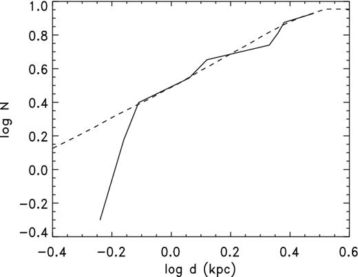
cdf for distance with C99 sample (filled circles) versus cdf for synthetic sample with linear distribution ( solid curve).
Table 7 shows how well B is estimated by both estimators with idealized synthetic samples similar to those used in Section 2.1. The actual value of B is 1.5, αS is 0.4, and dmax is 3000; the two are evaluated for a range of values of σlog d. The spatial distribution is the linear distribution appropriate to C99. In place of Γ, we have used Γ* ≡ dex(Γ) to make the comparison more directly.
Distance ratio estimates (with standard deviations) using κ, ζ and Γ* for different logarithmic uncertainties σlog d with B = 1.5.
| σlog d | κ | ζ | Γ* |
|---|---|---|---|
| 0.05 | 1.494 ± 0.006 | 1.379 ± 0.003 | 1.392 ± 0.003 |
| 0.075 | 1.488 ± 0.009 | 1.383 ± 0.010 | 1.396 ± 0.011 |
| 0.1 | 1.473 ± 0.008 | 1.376 ± 0.004 | 1.391 ± 0.004 |
| 0.125 | 1.459 ± 0.010 | 1.377 ± 0.012 | 1.394 ± 0.012 |
| 0.15 | 1.436 ± 0.006 | 1.371 ± 0.003 | 1.392 ± 0.002 |
As was noted above, the median σlog d for the C99 sample is 0.086 and the mean is 0.089. For those values, κ has less bias than ζ or Γ* and is roughly comparable in precision. The bias in κ is small for the relevant range in σlog d. As a matter of fact, both ζ and Γ* seem to have bias that is independent of σlog d, with Γ* having slightly less than ζ; for the given value of α, it is at most of order 7 and 8 per cent, respectively. Γ* is somewhat insensitive to outliers, though not quite as much as ζ. The bias in those two becomes smaller when α is reduced. In what follows, we will use κ and sometimes ζ in our comparisons of scales with C99.
For the C99 sample, the CKS distances give κ = 0.99 ± 0.07, with the error estimated using the jackknife method as before. ζ is virtually identical, 0.97 ± 0.09, which suggests no strong distance dependence is present. The median value of |${\cal R}_{{\rm CKS}}$| for C99 is 0.98, which agrees with κ and ζ. There are three of the eight values that are substantially smaller than unity and two substantially larger.
It appears that the CKS scale is in close agreement with the C99 distances, and were it not for the possibility of R dependence there would seem to be a contradiction with our result from H07. Fig. 5 shows a plot of |${\cal R}_{{\rm CKS}}$| from both the H07 sample and C99 as a function of log R. (The error bars for the C99 points are based, like those for H07, on αCKS = 0.35 but are combined with the estimated uncertainties for the spectroscopic parallaxes.) Clearly, |${\cal R}_{{\rm CKS}}$| decreases with increasing R, at least for medium to large nebulae. However, caution is called for because the displacement caused by a parallax error for H07 or a distance error for C99 follows a track very similar to the radius dependence in the distance ratio, as illustrated by the dashed curve which has been displaced to the upper right. As we will demonstrate below, correlated errors like those we have here with |${\cal R}$| and R connected through the standard distance dstd can distort a relation. Nevertheless, we will show in the next section that the dependence is real and is caused by the S–R relation used.
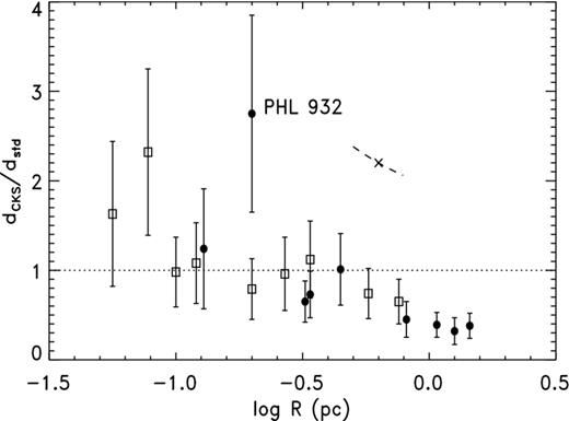
Concentrating on the range in log R over which the H07 and C99 samples overlap, namely −1 to 0, the distance ratios for the two – unweighted mean |${\cal R}_{{\rm CKS}} = 0.91\pm 0.14$| for H07 after correcting for sample selection bias, κ = 0.93 ± 0.07 for C99 – agree very well, which is encouraging. All but two of the C99 nebulae, K 1-27 and NGC 3132, are inside this range whereas only five H07 planetaries are. (K 1-27 does not have a CKS distance; also, it is a special case.). The mean log R for the H07 sample over this interval is −0.46 ± 0.13 while that for C99 is −0.59 ± 0.11.
The correlation coefficient r for the H07 distances compared to CKS is 0.55; that for C99 versus CKS is r = 0.93. A look at Fig. 7 (upper- left panel) of C99 confirms the correlation. Perhaps, the use of statistical distance as a confirmation criterion for central star companions accounts for some of the relatively high correlation with C99.
There are at least three reasons not to use the P96 spectroscopic parallaxes: (1) that data set was compiled from a variety of sources and is therefore not homogeneous; (2) the calibrations for the different sources may well depart from that for C99 and not necessarily be consistent with the latter or with H07 and (3) at this point we do not have error estimates, even approximate ones. This data set will be considered briefly in Section 3.3 and limited use made of it in Section 6.
Stanghellini, Shaw & Villaver (2008, hereafter SSV) revised the CKS scale using data on planetary nebulae in the Magellanic Clouds as well as Galactic calibration objects. Their scale is essentially identical to the CKS scale for optically thin nebulae; for optically thick planetaries, the slope of the relation between the optical thickness parameter τ (inversely proportional to Tb) and ionized mass parameter μ (proportional to Mi) is a little steeper, and the transition between the two is moved to a lower R value than with CKS. (A referee has pointed out that the φ values and fluxes from CKS were carried over by SSV, but see the exception noted below.) Our results for the CKS scale apply to the SSV scale as well because the distances from the two are virtually identical for the H07 and C99 samples, to within a factor of about 1.01. The lone exception is PuWe 1 from the H07 sample, whose SSV distance of 416 pc in their table 3 is incorrect; it should instead be 142 pc based on their calibration. (The error is traceable to truncation of the angular radius by the output format they used, which caused 1200 arcsec to be misread as 200 arcsec.) In particular, the same R-dependence as that of CKS is present.
3.3 The ‘long’ Z95 scale
Table 8 shows the distance values from Z95 for eight planetary nebulae in common with the H07 sample (and overlapping the CKS sample in Table 5) and eight in common with C99 together with the imposter PHL 932 as well as the individual distance ratios |${\cal R}_Z$| along with their estimated uncertainties |$\sigma _{\cal R}$|. As with CKS, the calculations do not include the latter object. The value chosen for αZ, 0.42, is higher than for CKS as explained below.
| Name | dZ (pc) | |${\cal R}_Z\pm \sigma _{\cal R}$| |
|---|---|---|
| A 7 | 700 | 1.04 ± 0.54 |
| A 21 | 710 | 1.31 ± 0.68 |
| A 24 | 1900 | 3.65 ± 1.68 |
| A 31 | 1010 | 1.63 ± 0.72 |
| NGC 6720 | 1130 | 1.60 ± 0.95 |
| NGC 6853 | 480 | 1.19 ± 0.50 |
| NGC 7293 | 420 | 1.96 ± 0.83 |
| PHL 932 | 3330 | 11.19 ± 5.21 |
| PuWe 1 | 900 | 2.47 ± 1.08 |
| A 33 | 2920 | 2.52 ± 1.14 |
| K 1-22 | 3430 | 2.58 ± 1.18 |
| Mz 2 | 2700 | 1.25 ± 0.62 |
| NGC 246 | 990 | 1.71 ± 0.86 |
| NGC 1535 | 2140 | 0.93 ± 0.43 |
| NGC 3132 | 1500 | 1.95 ± 1.16 |
| NGC 7008 | 1310 | 1.90 ± 0.95 |
| Sp 3 | 2620 | 1.10 ± 0.55 |
We estimate αZ using H07 in much the same way as before except that there is no bias from sample selection correlation as with CKS. For the synthetic T93 subsample, we use the values for uncorrelated distances. Six of the eight belong to that group; combining the values for the synthetic subsamples quadratically in that ratio when α = 0.35 we get |$\alpha _Z^\prime = 0.278$| and a ratio 0.79, while using our entire H07 synthetic sample we have 0.280 and ratio 0.8. The value of |$\alpha _Z^\prime$| from equation (5) is 0.342, so the above values indicate αZ is around 0.43.
The mean |${\cal R}_Z$| for the H07 planetaries is 1.85 ± 0.30 and the median 1.62. The weighted mean is 1.47 ± 0.22. Once again, the weighted mean is the smallest, presumably because of weighting bias. The expected weighting bias with αS = 0.42 is −0.60, some 60 per cent greater than the observed −0.38. The value of κ with C99 is 1.56 ± 0.26, while ζ is 1.62 ± 0.22; the uncertainties are estimated using the jackknife. The difference between H07 and C99 suggests there may be a radius dependence in the opposite direction from that for CKS, but in Fig. 6 there is no obvious trend of distance ratio with log R. In Section 5, we will confirm this dependence and explain why it exists.
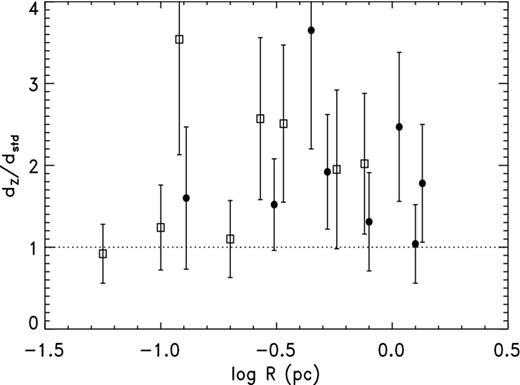
Clearly, |${\cal R}_Z$| for the H07 sample differs significantly from unity on average, and as a matter of fact not one individual value is less than or equal to unity (as H07 already found). The same is very nearly true of the C99 sample in the lower part of the table; only one value is less than unity, and that only slightly. Hence, we conclude that the Z95 scale is substantially overestimated. If we ignore for now the radius dependence, we can combine the H07 and C99 results to obtain a grand overall distance ratio for this scale. The uncertainties of the two estimated ratios are similar, the sample sizes are virtually the same, and the median relative errors are very nearly identical, so we simply weight them equally to arrive at a grand mean value, which is 1.71 ± 0.21. The ratio of the latter number to the CKS value 0.89 ± 0.08 (weighted mean of the ratios 0.72 and 0.99 we found for CKS in Sections 3.1 and 3.2) is quite close to the factor of 2 from Ph02 mentioned in the Introduction.
Overall, the H07 results are more or less consistent with the C99 ones in the region of overlap, as before taken to be −1 < log R (pc) ≤ 0. The mean distance ratio over this range with the H07 parallaxes is 1.94 ± 0.45, while κ for the C99 sample is 1.46 ± 0.29. The difference between the two values, while substantial, is smaller than the combined uncertainties.
The value of r for Z95 versus H07 is 0.39, even lower than for CKS. That for Z95 versus C99 is somewhat higher, 0.56, which is similar to what we found with CKS versus H07 but considerably lower than for CKS versus C99. Recall that the Z95 scale we have used is the mean of two scales, one based on Mi–R and the other on Tb–R. In Section 4, we consider the latter by itself.
3.4 F08, F14 mean Sα scale
Frew (F08) obtained a relation between Hα surface brightness Sα and R using a variety of calibrating objects. (He also obtained separate relations for several different types of nebulae; in this paper, we consider only the former because of the paucity of classifications.) In a recent paper Frew et al. 2014 (hereafter F14) have slightly revised that relation; Table 9 contains distances from table 2 of F14 derived using the mean relation and their distance ratios relative to H07 and C99. (Hereafter, unless we are referring to some other set of distances taken from F08 the ‘F08 scale’ is the scale based on the original mean Sα–R relation; other scales from F08 will have an identifier appended, and the same applies to F14.) Using our equation (5), we have found |$\alpha _{\rm F}^\prime$| to be 0.14 for F08 and 0.20 for F14. We have chosen to use the more conservative value of 0.20 for αF. (Hereafter in tables and in figure captions, we use the subscript ‘F’ to refer to F08 and ‘F*’ to refer to the F14 scale.)
| Name | d (pc) | |${\cal R}_{\rm F}*\pm \sigma _{\cal R}$| |
|---|---|---|
| A 7 | 590 | 0.87 ± 0.31 |
| A 21 | 450 | 0.83 ± 0.29 |
| A 24 | 900 | 1.73 ± 0.47 |
| A 31 | 460 | 0.74 ± 0.18 |
| A 74 | 620 | 0.82 ± 0.44 |
| NGC 6720 | 900 | 1.28 ± 0.57 |
| NGC 6853 | 310 | 0.76 ± 0.17 |
| NGC 7293 | 200 | 0.93 ± 0.19 |
| PuWe 1 | 390 | 1.07 ± 0.24 |
| Sh 2-216 | 80 | 0.62 ± 0.13 |
| Ton 320 | 480 | 0.90 ± 0.25 |
| A 33 | 1510 | 1.30 ± 0.33 |
| K 1-14 | 4980 | 1.66 ± 0.44 |
| K 1-22 | 1340 | 1.01 ± 0.27 |
| Mz 2 | 2010 | 0.93 ± 0.30 |
| NGC 246 | 770 | 1.33 ± 0.44 |
| NGC 1535 | 1740 | 0.75 ± 0.21 |
| NGC 3132 | 1100 | 1.42 ± 0.63 |
| NGC 7008 | 1000 | 1.44 ± 0.47 |
| Sp 3 | 2070 | 0.91 ± 0.31 |
The unweighted mean |${\cal R}_{\rm F}*$| for the H07 sample is 0.96 ± 0.09, the median is 0.87, and the weighted mean is 0.81 ± 0.07. The difference of −0.15 between the weighted and unweighted means, interpreted as weighting bias, is smaller than we found for CKS and Z95 but qualitatively consistent with our lower value for αF*. The value of κ for the C99 sample is 1.15 ± 0.06 and ζ is 1.15 ± 0.10; the uncertainty was estimated using the jackknife. Correlations of F14 with H07 and C99 are 0.78 and 0.83, respectively. The |${\cal R}_{\rm F}*$| values are plotted against log R in Fig. 7; there is no obvious trend but perhaps a drop in |${\cal R}_{\rm F}*$| at the largest R. In fact, as we demonstrate in Section 4.1 there appears to be a radius dependence similar to that with CKS but milder and over a smaller range. In Fig. 8, no distance dependence is evident.
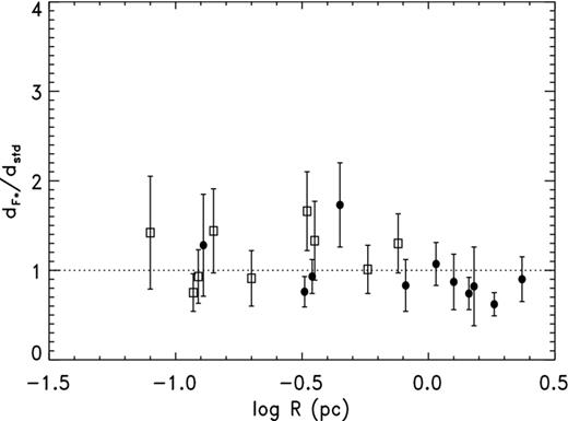
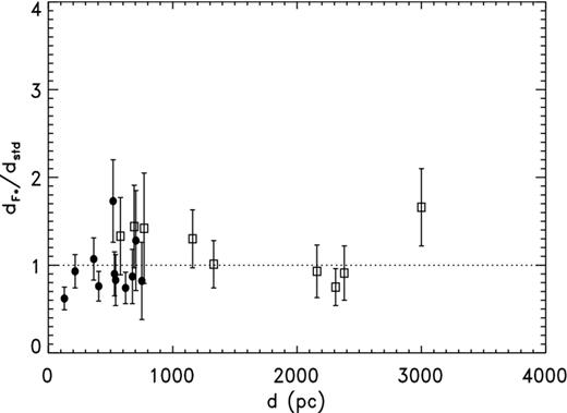
Combining the two values we have for the overall F14 distance ratio 1.01 ± 0.08, to be compared with 0.89 ± 0.08 for CKS and 1.71 ± 0.21 for Z95. (The respective correlations with F08 are r = 0.79 for H07 and 0.82 for C99.) Of course, H07 and C99 were given high weight in the F08 and F14 calibrations because of their (in most cases) small relative errors; on the other hand, F08 and F14 had large calibration sets (over 120 objects) and included many distances that we have rejected. Hence, we would not expect the overall distance ratio of nearly unity or the high correlation solely because of H07 and C99.
Using the F14 scale to indirectly compare H07 and C99 in the region of overlap, we find a mean |${\cal R}_{\rm F}$| for the former of 1.11 ± 0.18 and κ for the latter of 1.13 ± 0.17, confirming that the H07 and C99 distance scales are consistent with each other. Accordingly, C99 is treated as a primary distance standard on the same footing as H07.
There are no objects in common between the P96 spectroscopic parallaxes, termed here P96-s, and H07, but there are two with C99, namely NGC 246 and NGC 3132. For the former, the C99 distance is 1.2 times larger than the P96-s value, 580 pc versus 470 pc. With the latter, the C99 distance of 770 pc is more than 1.5 times larger than the P96-s value 510 pc.
The P96-s distances are compared with the F14 scale using κ and ζ as with C99. The distances for the six objects in common are shown in Table 10 together with the distance ratios. The overall F14/P96 distance ratio is κ = 2.26 ± 0.35; the same with ζ. In almost every case except He 2-36, the distance ratio is equal to or not far from 2.00, indicating a calibration problem. The correlation between P96-s and F14 is fairly high, namely 0.90. The mean value is larger than that for F14/C99 by very nearly a factor of 2, and the difference is clearly statistically significant. It is also larger than the F14/H07 value, by a factor of more than 2. These findings imply that the P96-s distances can be used provided the distances are doubled and we choose a reasonable value for αP. Unfortunately, we are unable to estimate αP directly from this comparison, but the high correlation with F14 together with the relatively small αF suggests that it is not large.
| Name | dP, s | dF | |${\cal R}_{{\rm F}*/P}$| |
|---|---|---|---|
| He 2-36 | 780 | 2640 | 3.38 |
| LoTr 5 | 420 | 910 | 2.17 |
| NGC 246 | 470 | 770 | 1.64 |
| NGC 1514 | 400 | 650 | 1.63 |
| NGC 2346 | 690 | 1340 | 1.94 |
| NGC 3132 | 510 | 1100 | 2.16 |
| Name | dP, s | dF | |${\cal R}_{{\rm F}*/P}$| |
|---|---|---|---|
| He 2-36 | 780 | 2640 | 3.38 |
| LoTr 5 | 420 | 910 | 2.17 |
| NGC 246 | 470 | 770 | 1.64 |
| NGC 1514 | 400 | 650 | 1.63 |
| NGC 2346 | 690 | 1340 | 1.94 |
| NGC 3132 | 510 | 1100 | 2.16 |
| Name | dP, s | dF | |${\cal R}_{{\rm F}*/P}$| |
|---|---|---|---|
| He 2-36 | 780 | 2640 | 3.38 |
| LoTr 5 | 420 | 910 | 2.17 |
| NGC 246 | 470 | 770 | 1.64 |
| NGC 1514 | 400 | 650 | 1.63 |
| NGC 2346 | 690 | 1340 | 1.94 |
| NGC 3132 | 510 | 1100 | 2.16 |
| Name | dP, s | dF | |${\cal R}_{{\rm F}*/P}$| |
|---|---|---|---|
| He 2-36 | 780 | 2640 | 3.38 |
| LoTr 5 | 420 | 910 | 2.17 |
| NGC 246 | 470 | 770 | 1.64 |
| NGC 1514 | 400 | 650 | 1.63 |
| NGC 2346 | 690 | 1340 | 1.94 |
| NGC 3132 | 510 | 1100 | 2.16 |
4 THE BRIGHTNESS TEMPERATURE–RADIUS RELATION
4.1 The Tb–R relation
We have Tb for a number of the H07 and C99 nebulae based on published 5 GHz flux densities from A92 and Z95. For several objects, the Tb values given in table 3 of Z95 are inadequate because they are only given to two decimal places; this is of course particularly a problem for the larger nebulae. We have recalculated those, and the logarithms of the new values are included in Table 11. The φ values used in the calculations are those from Tables 1 and 6 for the sake of consistency.
| Name | S5 (mJy) | Ref. | log Tb (K) |
|---|---|---|---|
| A 7 | 305.0 | Z95 | −1.43 |
| A 21 | 327.0 | A92 | −1.21 |
| A 24 | 36.0 | Z95 | −1.69 |
| A 31 | 101.9 | Z95 | −2.12 |
| A 33 | 14.0 | Z95 | −1.87 |
| K 1-22 | 11.5 | Z95 | −1.60 |
| Mz 2 | 75.0 | A92 | 1.00 |
| NGC 246 | 248.0 | Z95 | −0.46 |
| NGC 1535 | 160.0 | Z95 | 1.52 |
| NGC 3132 | 230.0 | Z95 | 1.26 |
| NGC 6720 | 360.0 | Z95 | 0.72 |
| NGC 6853 | 1325.0 | Z95 | −0.06 |
| NGC 7008 | 217.0 | A92 | 0.32 |
| NGC 7293 | 1292.0 | A92 | −0.68 |
| PHL 932 | 10.0 | Z95 | −2.03 |
| PuWe 1 | 84.7 | Z95 | −2.38 |
| Sp 3 | 61.0 | A92 | 0.53 |
Our log R values based on H07 and C99 are graphed against the log Tb values in Fig. 9. R for NGC 6720 has been corrected slightly for the Lutz–Kelker effect discussed in Section 2.2; in the other cases, the correction was deemed insignificant and has been omitted. PHL 932, HDW 4 and DeHt 5 are included for illustrative purposes along with K 1-27 from C99; they were not used in any of the least-squares solutions presented in Table 12. H07 and C99 define fairly similar Tb–R relations. As expected, the imposters’ statistical distances would be overestimated. K 1-27 may be an outlier because of an incorrect spectroscopic parallax, but we consider it more likely because it is not a typical planetary nebula.
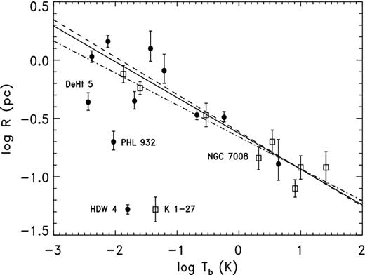
Values for intercept e and slope f for the Tb–R relation obtained by various authors and correlation coefficient r.
| e | f | r | Ref. |
|---|---|---|---|
| −0.56 ± 0.05 | −0.32 ± 0.02 | −0.80 | Z95-Tb |
| −0.33 ± 0.08 | −0.42 ± 0.05 | −0.85 | Z95-Mi |
| −0.51 ± 0.05 | −0.35 ± 0.02 | −0.84 | VdSZ |
| −0.35 | −0.39 | −0.90 | BL01 |
| −0.86 ± 0.03 | −0.36 ± 0.02 | Ph02, |$d_p^*\le 1$| kpc | |
| −0.63 ± 0.04 | −0.27 ± 0.03 | Ph02, dp >1 kpc | |
| −0.66 ± 0.10 | −0.33 ± 0.07 | −0.82 | H07, this paper |
| −0.71 ± 0.06 | −0.29 ± 0.05 | −0.92 | C99, this paper |
| −0.68 ± 0.05 | −0.32 ± 0.04 | −0.93 | H07+C99 |
| −0.64 ± 0.09 | −0.24 ± 0.04 | −0.89 | LMC |
| −0.53 ± 0.25 | −0.29 ± 0.11 | −0.92 | SMC |
*The projected distance dp is given by d · cos b, with b the galactic latitude.
Using equations (1), (3), (4) and (5) in Z95 and assuming a constant filling factor ϵ = 0.6, the Mi–R relation yields a Tb–R relation with e = −0.33 and f = −0.42 as given in Table 12. As a result of the difference in their Tb–R relations, the two distance scales that are combined to give the Z95 mean distances have a Tb-dependent difference which can be discerned in table 3 of Z95. Specifically, the steeper slope for the Z95–Mi relation introduces a growing overestimation of distance with increasing R, the opposite of CKS and SSV. The expected distance ratio [mean/Tb] increases from roughly unity at small R to a factor of 2.2 for R = 2 pc.
The slope of the Z95,Tb–R relation is very close to that for H07 and C99 together, suggesting that the scale based on it, termed Z95-Tb, might be nearly free of radius dependence. The value of |$\alpha _{Z,T}^\prime$| found for the Z95-Tb distances with the H07 sample is 0.281, very close to the value quoted in Z95 but lower than the value we found earlier for the mean Z95 scale. Correcting based on the H07 synthetic sample as for the mean Z95 case, we estimate αZ, T to be 0.35. Comparison with C99 gives a much lower |$\alpha ^\prime _{Z,T}$|, namely 0.12, but such a low value is highly implausible. We thus adopt the value 0.35. The unweighted mean |${\cal R}_{Z,T}$| for H07 is 1.12 ± 0.16, the weighted mean is 0.91 ± 0.14, the median is 1.00 and the correlation is 0.51. With C99, we find κ = 1.13 ± 0.11 and ζ = 1.21 ± 0.11; the median is somewhat larger, 1.30. The correlation is 0.88. Distance ratios are presented in Table 13. Fig. 10 indicates no radius dependence with Z95-Tb, and Fig. 11 shows no distance dependence.
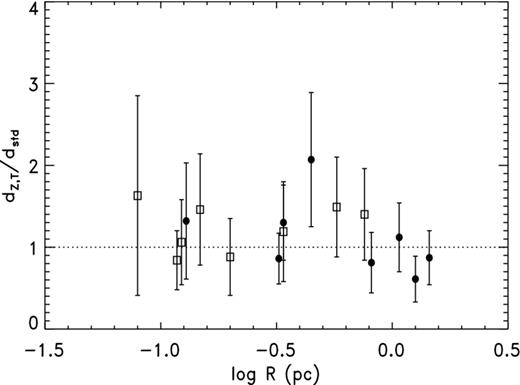
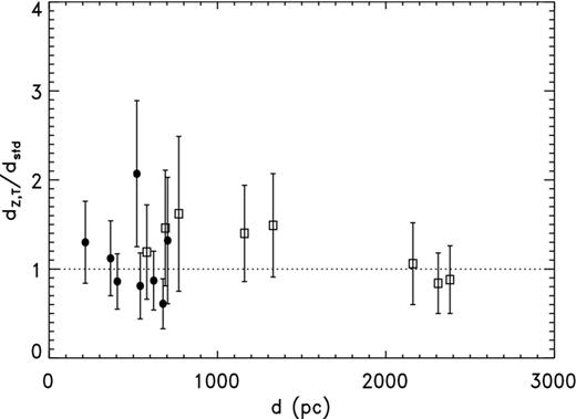
| Name | dZ, T (pc) | |${\cal R}_{Z,T}\pm \sigma _{\cal R}$| |
|---|---|---|
| A 7 | 410 | 0.61 ± 0.28 |
| A 21 | 440 | 0.81 ± 0.37 |
| A 24 | 1080 | 2.07 ± 0.82 |
| A 31 | 540 | 0.87 ± 0.33 |
| NGC 6720 | 930 | 1.32 ± 0.71 |
| NGC 6853 | 350 | 0.86 ± 0.31 |
| NGC 7293 | 280 | 1.30 ± 0.46 |
| PHL 932 | 1790 | 6.01 ± 2.80 |
| PuWe 1 | 410 | 1.12 ± 0.42 |
| A 33 | 1620 | 1.40 ± 0.54 |
| K 1-22 | 1980 | 1.49 ± 0.58 |
| Mz 2 | 2290 | 1.06 ± 0.46 |
| NGC 246 | 690 | 1.19 ± 0.53 |
| NGC 1535 | 1940 | 0.84 ± 0.34 |
| NGC 3132 | 1250 | 1.62 ± 0.87 |
| NGC 7008 | 1010 | 1.46 ± 0.65 |
| Sp 3 | 2090 | 0.88 ± 0.38 |
Comparison of the Z95-Tb scale with F14 gives κ = 1.03 ± 0.02 and ζ = 1.02 ± 0.02. The correlation r is 0.78. Fig. 12 shows the distance ratio for Z95-Tb/F14 as a function of RF*, and Fig. 13 shows the ratio as a function of dF*. In our judgment the Z95-Tb scale is good enough to serve as a standard.
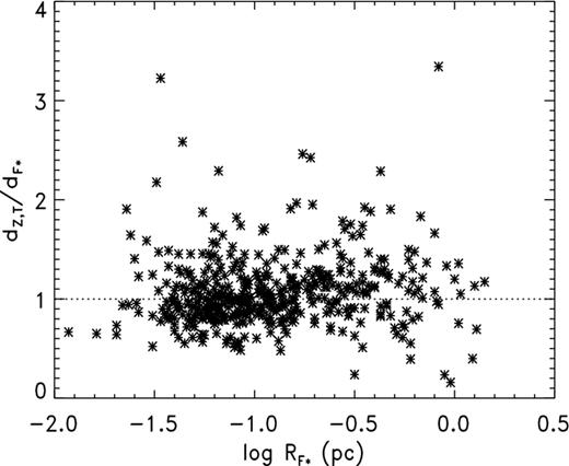
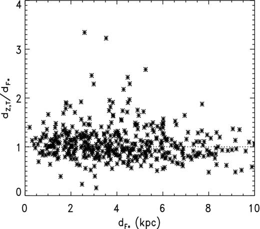
The Mi–R relation implies such a different slope because of how it was calibrated. In Fig. 14, we present synthetic data for a large (N = 8000) sample of planetaries all of which are assumed to obey the mass–radius relation Mi = M0(R/R0)0.9 with M0 = 0.2M⊙ and R0 = 0.122 pc. The apparently arbitrary choice for the exponent comes from a least-squares fit of revised Mi values to Ri values, both corrected using the F08 distances. Each value of Mi from the Z95 calibration was multiplied by the 2.5 power of the ratio of F08 distance to Z95 calibration distance, based on equation 4 of Z95, and the corresponding R was multiplied by the distance ratio. The logarithmic slope found by least squares was 0.91 ± 0.08 instead of the value 1.31 ± 0.07 from equation 5 in Z95; although our value is probably closer to the true slope because of the more accurate F08 distances it may well still be slightly too high. The ‘true’ R values for the synthetic sample were selected at random over the interval 0.05–0.5 pc; random (Gaussian) relative errors in R (corresponding to errors in distance) with standard deviation α = 0.35 were then added to give ‘measured’ values R′. The ‘calculated’ value of Mi, which we call |$M_{\rm i}^\prime$|, was obtained using the same equation, multiplying Mi by (R′/R)2.5. Least-squares fitting of log |$M_{\rm i}^\prime$| to log R′ yields a value 1.31 ± 0.01 for the logarithmic slope of the Mi–R relation, and the correlation is r = 0.89. Clearly correlation of the errors in Mi and R tends to steepen the relation.
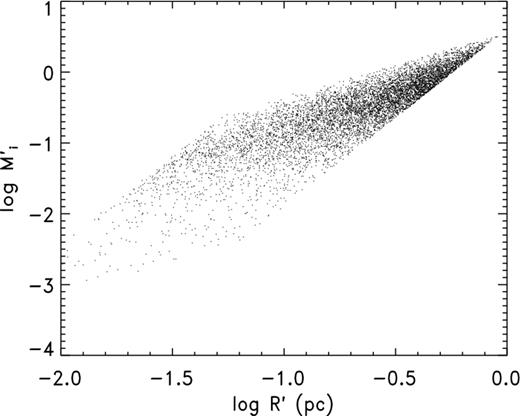
Log of simulated ionized mass |$M_{\rm i}^\prime$| versus log R′ for synthetic data (N = 8000) (see text for recipe).
Our finding for the Z95-Mi scale coincidentally sheds new light on the first ‘long’ statistical scale known to us. Seaton's original calibration in S66 for optically thin nebulae was based on estimation of Mi, which (as was customary at the time) he took to be constant. He used measures of the [O ii] λ3727 Å line pair to estimate the quantity |$x\equiv N_{\rm e}\ T_{\rm e}^{-1/2}$| for each of 14 calibration nebulae; as usual Ne is the electron temperature and Te the electron temperature. Using the x value and the ϵ value estimated from photographs together with the Hβ surface brightness, he could then obtain a value for the radius, R(Ne) (see equation 6 of S66). The nebular mass Mi can then be shown to be proportional to the quantity R3(Ne)ϵx. Eight objects were identified as optically thin on spectroscopic grounds, but two including NGC 2392 were ignored because of small R(Ne) and hence small R3(Ne)ϵx (cf. fig. 1 of S66).
A problem with the S66 approach is that, like Mi and R in Z95, the quantities R(Ne)3ϵx and R(Ne) have correlated errors because they depend on (mostly) the same quantities. Errors in distance cause errors in R which tend to move a data point along a line of slope 3; R3(Ne)ϵx is highly sensitive to those. Similar correlations arise from errors in ϵ and x because they are elements of the estimation of R and hence distance in S66. As a result, modest errors cause large deviations which could remove an object from inclusion in the mean. A striking illustration of this is NGC 2392. The S66 value for log x was −0.11; Kingsburgh & Barlow (1992) found it to be −0.89. In consequence, the value of log R(Ne) changed from −1.86 to −0.77 and R3(Ne)ϵx changed from −6.99 to −3.72, placing NGC 2392 in the midst of the calibration nebulae. Correcting the S66 values using F08 or, for NGC 6210 and HD 138403, Z95-Tb, we find the S66 distance scale is reduced by 31 per cent.
The radius dependence of |${\cal R}_{{\rm CKS}}$| obviously results from an incorrect value for the logarithmic slope of the S–R and Tb–R relations for the larger nebulae. The CKS and SSV value of f for optically thin nebulae is the original Shklovsky value −0.2, which causes distances to be increasingly underestimated as S and Tb decrease and R increases, the radius dependence seen in Fig. 5. This problem was already noted in F08.
Thus far, our Tb–R relation includes only nebulae having log R ≥ −1.2. There is a considerable body of data on Magellanic Cloud planetaries (Shaw et al. 2001, 2006; Stanghellini et al. 2002, 2003). Table 12 contains the values of e and f from least-squares fit to these data also. The two samples are at reasonably well-known distances and can used to calibrate statistical scales, as SSV stated. Although those authors recommend using the photometric radius, for consistency with our results we chose the geometric mean of the two optical dimensions to obtain the results in Table 12. We have calculated Tb using equation (6) from CKS to convert FHβ to S5 (in mJy). Only those nebulae having extinction values c were included.
From the table, we see that f for the Large Magellanic Cloud (LMC) sample is closer to the Shklovsky value than either our standard samples or the SMC one. In Fig. 15, we have added Magellanic Cloud (MC) data to our Fig. 9. Those data appear to match up with our H07–C99 relation where they overlap. Also shown for reference are lines schematically representing three evolutionary stages: a dotted line with f = −0.33, a dashed line with f = −0.2 and a solid line having f = −0.5. In F14, the Sα–R relation in equation 13 implies a slope of −0.275, slightly less steep than we find for C99. (The slope in F08 is −0.277.) That value is roughly midway between −0.2 and −0.33; a single line with that slope would fit well too. In Table 12, there is a trend of f decreasing with decreasing Tb, but the differences are not statistically significant.
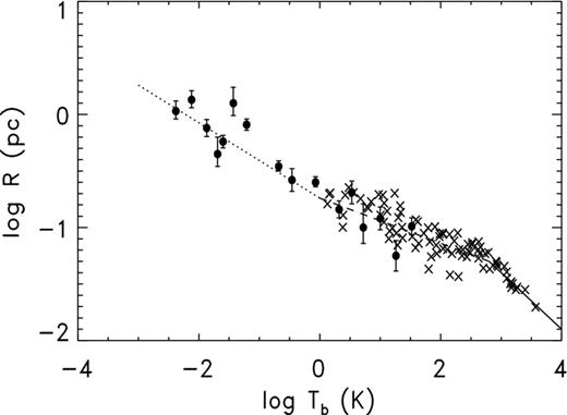
Schneider & Buckley (1996) proposed a quadratic form for the (logarithmic) Tb–R relation rather than a single power law. However, their formula explicitly approached the Shklovsky slope at large R, whereas we find a steeper slope there.
We have estimated the rms relative error in R(Tb), essentially αMC, from the least-squares fit for the two MC samples. Nebulæ having log Tb > 2.8 seem to lie on a tightly constrained line and are presumably optically thick; leaving those out we find 0.31 and 0.27. These values are only upper limits to the intrinsic spread for a mixture of types.
To examine possible underestimation at large R with the Frew Hα scale, we first look at Sα instead of Tb as shown in Fig. 16. We find least-squares slopes with H07 and C99 of −0.31 ± 0.03 and −0.28 ± 0.03, respectively, more precise than those in Table 12 but basically the same (and consistent with the F08 and F14 slopes). All of the largest (i.e. lowest Sα) objects lie on or above the dotted line corresponding to the mean relation from F14. Secondly, comparing the calibration distances from table 7.1 of F08 with those predicted by the F08 mean relation, we find that of the 37 nebulae with log RF > −0.4 the nine largest, with +0.05 < log RF, have Hα distances that are underestimated, by as much as a factor of slightly more than 2. Fewer than half of these are H07 objects. The mean distance ratio for the nine is 1.52 ± 0.11 compared to 0.95 ± 0.07 for the remainder. The result for F14 with 11 nebulae larger than the limit taken from table 1 is similar but generally smaller, with mean 1.38 ± 0.09 and largest ratios 1.87. Hence, the Hα distances appear to be underestimated by a factor of roughly 1.5 for log RF > +0.05. This factor is to be compared to the corresponding CKS value of 2.5 for the three nebulae in Fig. 5 with log R > 0 (roughly equivalent in our system to log RF = +0.05). This underestimation with the F14 relation is visible in figs 2 and 4 of F14 and was mentioned there.
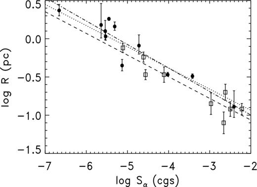
4.2 The Tb–R relation and nebular evolution
Traditionally, the S–R relation and the Tb–R relation have been thought to reflect in a gross sense the evolution of the nebula. Recently, this evolution has been described in some detail by Jacob, Schönberber & Steffen (2013), based on hydrodynamical modelling coupled to the evolution of the central star. The authors found that their models agree well with the F08,Sα–R relation and with the Magellanic Cloud relation presented in F08 (cf. their fig. 4). The same may be said of the F14 relation; see fig. 4 of that paper.
Our results seem mostly consistent with these. The Jacob et al. tracks stop at R = 1 pc, so they do not show the steepening slope at large R or the F08/F14 underestimation. (The figure uses F08's definition of radius, which differs a little from ours.) In our Fig. 15, there is also steepening at small R for the Magellanic sample where the nebulae are optically thick. The model tracks show a flattening, qualitatively the same as our steepening because the axes are reversed. The points for log Tb > 2.8 in Fig. 14 are few but fit tightly around a line of slope f ≃ −0.5. In F14, a theoretical value corresponding to f = −0.61 is given for the optically thick case.
We have looked at the ISM interaction classes of Wareing, Zijlstra & O'Brien (2007) for the H07 and C99 objects in Fig. 9. The range is from WZO 1 to 2; none of these are class 2/3 or 3. Class 2 is unsurprisingly to be found almost entirely among some of the larger objects, but some of those are 1/2 or even 1. For instance, A 7, one of the largest, is class 1. In Fig. 15, the very largest objects, Ton 320 and Sh 2-216, are the only ones classified as having strong interaction with the ISM, as might have been expected; their WZO classes are 3 and 2/3, respectively. The interaction is expected to cause a brightening, but we do not see that for Ton 320, apparently the one most strongly affected. However, its angular diameter is not from A92. Possibly, Sh 2-216 has been affected, but it is situated near a clump of nebulae with lower classes. On the other hand, the environments may differ among these.
5 GRAVITY, EXPANSION AND EXTINCTION DISTANCES
5.1 Gravity distances
The largest truly homogeneous set of gravity distances known to us is that of N01 for hydrogen-rich central stars of old planetaries. Because they are old and hence fairly large these nebulae more nearly resemble those of the H07 sample than the ones in the C99 sample; indeed, no C99 object is in the set. Data for the eleven H07 central stars having N01 distances are in Table 14. Also included are spectral types from Napiwotzki & Schönberner (1995, hereafter NS95). The sample includes PHL 932, DeHt 5 and HDW 4, which are imposters; however, that fact is irrelevant here because no assumed value of Mi plays a role in gravity method distances. PHL 932 does not have an anomalously large distance ratio, instead the smallest. DeHt 5 and HDW 4 have ratios comfortably inside the range of the others.
| Name | Spectral type | dN (pc) | |${\cal R}_N\pm \sigma _{\cal R}$| |
|---|---|---|---|
| A 7 | DAO | 700 | 1.04 ± 0.66 |
| A 31 | – | 1000 | 1.61 ± 0.76 |
| A 74 | DAO | 1700 | 2.26 ± 1.38 |
| DeHt 5 | DA | 510 | 1.48 ± 0.45 |
| HDW 4 | DA | 250 | 1.20 ± 0.36 |
| NGC 6720 | DA | 1100 | 1.56 ± 0.80 |
| NGC 6853 | sdO/DAO | 440 | 1.09 ± 0.34 |
| NGC 7293 | DAO | 290 | 1.35 ± 0.37 |
| PHL 932 | hgO(H) | 240 | 0.81 ± 0.21 |
| PuWe 1 | DAO | 700 | 1.92 ± 0.65 |
| Sh 2-216 | DAO | 190 | 1.47 ± 0.36 |
The median relative error for the entire N01 sample calculated from the stated uncertainties is 0.30, slightly less than for the CKS scale (0.35). We consider this a lower bound to αN and will instead adopt the value 0.35. In our analysis, we treat the uncertainties as symmetric even though they are not, as though the pdf were normal. While not rigorous, this treatment probably makes little difference in our results.
The mean |${\cal R}_N$| with all objects included is 1.43 ± 0.12. The median is slightly larger, 1.47. The weighted mean including all objects is 1.23 ± 0.13. Again, it is likely that the difference is attributable to weighting bias; our H07 model predicts −0.29 for αS = 0.3. There must be a fairly large overestimation relative to the H07 distances: Of the 11 objects, only PHL 932 has |${\cal R}_N<1$|.
The degree of overestimation seems unrelated to spectral type. The cause of such a distance overestimation is unlikely to lie with either M* or Fλ5480; in either case that is improbable. (For the latter, it would mean overestimating Teff by a factor 2.) If overestimation of both were to blame, at least one would have to be at least 40 per cent too high. One can easily imagine log g being systematically too small by something like 0.20. Indeed, in both P96 and B09, it was suggested that log g is responsible. Fig. 17 hints at R dependence, with the highest |${\cal R}_N$| at R > 1 pc. However, the sample is small and the errors are large.
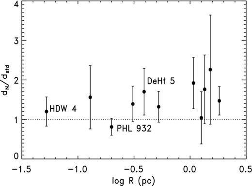
The N01 scale is also tested using the F14 scale as intermediary; leaving out objects that are not planetaries there are 19 nebulae in common. Unlike H07, the F14 sample includes smaller nebulae and some that are distant. We find κ = 0.98 ± 0.14 and ζ = 1.23 ± 0.15. The differences between |${\cal R}_N$| and ζ and between κ and ζ indicate a distance dependence while the former difference also suggests a possible radius dependence.
Fig. 18 is a plot of the N01/F14 distance ratio as a function of the F14 distance dF*. The overestimation is entirely for planetaries with dF* < 1 kpc and hence consistent with our finding for H07. At larger dF*, there seems to be underestimation, and κ weights larger distances more heavily, which we believe to be the reason for the difference between κ and ζ. With κ, the low distance ratios at 2–3 kpc almost cancel the high ones inside 1 kpc; if there were a few more nebulae out there it would have. With ζ, the ratios are weighted more evenly, but the value is lower than for H07 most obviously because it includes the underestimates at large distances. The low distance ratios at large dF* with this sample may partly be due to positive errors in the F14 distances. However, considering the fairly high precision of F14 we do not expect errors to contribute so much in the way of overestimation, and the difference between |${\cal R}_N$| and ζ argues against that explanation. The central star of HDW 11 which is not a post-AGB object is marked as such in this figure as well as Fig. 20.
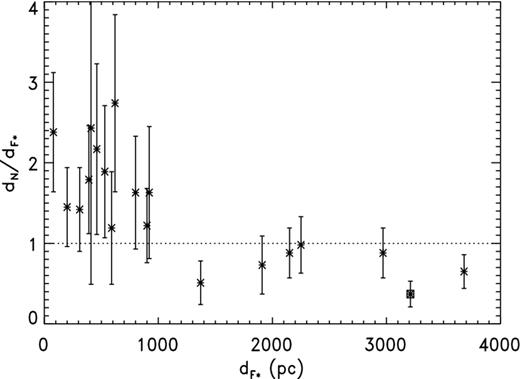
The effect of scatter in the standard distances, for example with F08 or F14, is shown in Fig. 19 using synthetic data (N = 8000). This example was based on an exponential space distribution like that of N01 with scaleheight z0 = 250 pc, distance scale factor B = 1.5 (roughly the value for N01 versus H07), α1 = 0.20 (for both F08 and F14) and α2 = 0.3, and a distance cut-off of 2 kpc. (Remember that the F08 sample in table 9.4 is basically truncated at that value.) The filled circles are means in bins of 0.2 kpc. Note the elevation of d2/d1 at small d1 and the depression at large d1. The former is associated with negative errors in d1; because of the geometry more objects will be scattered in by those than are scattered out by positive errors. Comparison with Fig. 18 suggests that the effect at large d1 is insufficient to explain the behaviour of the real sample. There are only a few data points, but it seems to us that there is a real distance dependence with N01. If so, we cannot explain it.
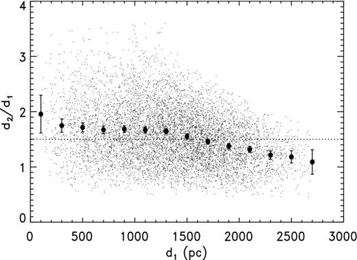
Distance ratio d2/d1 versus d1 for synthetic data with true ratio B = 1.5; see text.
Fig. 20 shows the ratio dN/dF* as a function of log RF*. (Recall that the F08 φ values tend to be a little larger than those used with H07 and C99, about 0.05 in the log, so the RF* values will likewise tend to be that much larger.) The most severe overestimation appears to be mainly at large R; the mean distance ratio is 2.03 for RF* > 1 pc versus 0.97 for the smaller objects. However, many of the latter have dF* > 1 kpc while none of the former do, so distance dependence accounts for some of the difference. As we showed in Section 4.1, there is underestimation of distance for R > 1 pc with the Hα scale that can qualitatively explain the larger apparent degree of overestimation seen in the figure than in Fig. 17. There is thus no persuasive evidence of R dependence with N01.
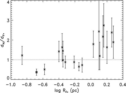
Considering dN/dstd as a function of V for just the objects with standard distances less than 1 kpc, we see signs of an increase going to fainter stars. For the four brightest stars, with V < 15, the weighted mean distance ratio is 1.06 ± 0.15; for the nine stars with 15 < V < 17 it is 1.26 ± 0.16; while for the four faintest stars (17 ≤ V < 18) it is 2.08 ± 0.57. Breaking the ratios down according to MV instead, we have a ratio for the three brightest stars of 0.94 ± 0.16, for the eleven stars with MV between 6 and 8 1.40 ± 0.16, and for the three faintest stars 1.36 ± 0.33. Thus, the effect seems to depend primarily on V rather than MV, raising suspicion of some observational effect.
The correlation coefficient for the N01 and H07 distances is 0.89; for the N01 and F14 distances, it is 0.77. Since we believe the precision of F14 is comparable to that of the original H07 parallaxes, we conjecture that the larger typical distances for the F14 nebulae along with the possible N01 distance dependence may weaken the correlation in the latter case.
A compilation of gravity distances with estimated uncertainties is in table 5 of F14. The unweighted mean distance ratio for the F14-g distances compared to H07 (N = 10) is 1.32 ± 0.15 and the weighted mean 1.14 ± 0.16; the difference is presumably due to weighting bias. The value of κ for the two C99 objects, NGC 246 and NGC 1535, is 0.96. The median distance ratio for all 12 is 1.26, and only three have ratios less than unity. On the other hand, only one is more distant than 1 kpc. Comparing the F14-g distances with the F14 ones (N = 58) we find that κ = 0.81 ± 0.06 and ζ = 0.95 ± 0.05. Looking at the distance ratio as a function of distance (Fig. 21), we see a pattern similar to that for N01, namely overestimation for d < 1 kpc and (more clearly) underestimation beyond. Note that this figure and Fig. 22 include F14 data. There might be overestimation at large R, but it is hard to tell.
Table 6 of P96 was a compilation of mean gravity distances from various sources, so it is strictly speaking inhomogeneous; however, the vast majority are from the Rauch–Werner group. We denote these by P96-g. It includes 13 of the H07 objects and two from C99. Some involve earlier distances from Napiwotzki (1993) and thus may not be independent of N01. Errors have been estimated using αP, g = 0.35; with H07 equation 5 gives |$\alpha _{P,g}^\prime = 0.14$| (far too low in our opinion) while equation 8 with F08 yields |$\alpha _{P,g}^\prime = 0.30$|. The mean distance ratio for the H07 objects is 1.15 ± 0.09 and the weighted mean 0.99 ± 0.10, with a small weighting bias. For the two C99 objects, κ = 1.02. Nine of the 15 have ratios greater than unity, indicating little if any overestimation. For the F14 distances (N = 28) we find κ = 0.80 ± 0.07 and ζ = 0.90 ± 0.07. The median dP, g/dF* is 0.84, with 18 of 28 ratios less than unity; hence there may be a slight underestimation overall. We see no indication of R dependence. Looking at the ratio as a function of dF* (Fig. 23), there is a pattern like that of N01 but weaker. The correlation r with H07 is 0.84, that with C99 is 0.83, and for F14 it is 0.82.
There is independent evidence that error in log g can cause overestimation. Some central stars of planetaries are PG 1159 type, for example that of NGC 246. For the GW Vir stars, a subset of that class that are non-radial pulsators, g can be estimated using asteroseismology. Table 6 of Córsico & Althaus (2006) compares spectroscopic estimates of Teff, M* and log g with those from models that fit the pulsations for four ‘naked’ GW Vir stars (those without nebulae). The spectroscopic g's are all smaller, by average Δlog g of −0.25 ± 0.06. The differences in log Teff are negligible (mean Δlog Teff = −0.04 ± 0.05); the mean Δlog M* is −0.04 ± 0.01. Applying equation (10), we find that these differences imply Δlog d = 0.11, which corresponds to a distance overestimation of a factor 1.29. However, asteroseismology involves modelling; in addition, the average spectroscopic log g for these high-gravity GW Vir stars is 7.38, higher than 49 of the 60 values in table 6.6 of F08 and 24 of 27 in table 2 of N01. One does not know whether the same effect might occur at lower g.
5.2 Expansion distances
Two homogeneous samples of expansion distances obtained using HST are considered. The first is tiny, consisting of but three objects imaged and measured by Palen et al. (2002). The second is a sample of 15 nebulae measured by Hajian and collaborators and analysed by F08; the results for these after the latter's application of his own values of F are taken from his table 6.5. We refer to this as the Hajian–Frew sample.
The Palen et al. expansion distances are compared with the F14 distances in Table 15. They were derived using velocities Vm given in that paper instead of catalogue values. Rather than combine the results from the gradient and magnification methods (described in the reference), we have kept them separate. The unweighted mean Fg for the gradient method is 1.78 ± 0.15, which is higher than one might expect; that for the magnification method is Fm = 1.52 ± 0.20, closer to the conventional 1.35 (cf. S05). The F08 distances are lower, giving respective means of 1.57 ± 0.10 and 1.35 ± 0.23.
| Name | dF (pc) | Fg ± σF | Fm ± σF |
|---|---|---|---|
| IC 2448 | 2470 | 1.83 ± 0.93 | 1.89 ± 0.64 |
| NGC 6578 | 2290 | 1.50 ± 0.85 | 1.23 ± 0.40 |
| NGC 6884 | 2420 | 2.02 ± 1.34 | 1.43 ± 0.39 |
| Name | dF (pc) | Fg ± σF | Fm ± σF |
|---|---|---|---|
| IC 2448 | 2470 | 1.83 ± 0.93 | 1.89 ± 0.64 |
| NGC 6578 | 2290 | 1.50 ± 0.85 | 1.23 ± 0.40 |
| NGC 6884 | 2420 | 2.02 ± 1.34 | 1.43 ± 0.39 |
| Name | dF (pc) | Fg ± σF | Fm ± σF |
|---|---|---|---|
| IC 2448 | 2470 | 1.83 ± 0.93 | 1.89 ± 0.64 |
| NGC 6578 | 2290 | 1.50 ± 0.85 | 1.23 ± 0.40 |
| NGC 6884 | 2420 | 2.02 ± 1.34 | 1.43 ± 0.39 |
| Name | dF (pc) | Fg ± σF | Fm ± σF |
|---|---|---|---|
| IC 2448 | 2470 | 1.83 ± 0.93 | 1.89 ± 0.64 |
| NGC 6578 | 2290 | 1.50 ± 0.85 | 1.23 ± 0.40 |
| NGC 6884 | 2420 | 2.02 ± 1.34 | 1.43 ± 0.39 |
We do not estimate F for the Hajian–Frew HST expansion distances because it has already been taken into account; also, we do not have the angular expansion rates. To evaluate these distances overall, we use κ and ζ. Since there are F08 distances for only eight of them, we use distances from F14 and Z95-Tb. Table 16 shows the individual distance ratios. The uncertainties given are combinations of the respective α's with the individual values of relative error according to F08. The median of those is 0.22, whereas using equation (8) with the F14 distances yielded |$\alpha _{H{\rm -}F}^\prime = 0.26$| and with the Z95-Tb distances 0.35. It thus appears that these distances are not as precise as the H07, C99, F08 and F14 ones but perhaps a little more so than Z95-Tb.
| Name | |${\cal R}_{H{\rm -}F}$| (F14) | |${\cal R}_{H{\rm -}F}$| (Z95-Tb) | ||
|---|---|---|---|---|
| BD+30° 3639 | 0.60 ± 0.15 | 0.64 ± 0.24 | ||
| =He 2-438 | ||||
| IC 418 | 0.85 ± 0.23 | 0.93 ± 0.36 | ||
| IC 2448 | 0.85 ± 0.26 | 0.69 ± 0.29 | ||
| J 900 | 1.24 ± 0.36 | 1.42 ± 0.58 | ||
| NGC 3132 | 1.09 ± 0.42 | 0.96 ± 0.46 | ||
| NGC 3918 | 0.96 ± 0.28 | 1.18 ± 0.48 | ||
| NGC 5882 | 0.89 ± 0.27 | 1.01 ± 0.42 | ||
| NGC 5979 | 0.72 ± 0.23 | 0.69 ± 0.30 | ||
| NGC 6326 | 1.80 ± 0.57 | 1.78 ± 0.77 | ||
| NGC 6543 | 1.36 ± 0.45 | 1.35 ± 0.59 | ||
| NGC 6565 | 0.81 ± 0.23 | 0.64 ± 0.26 | ||
| NGC 6826 | 1.69 ± 0.53 | 3.00 ± 1.26 | ||
| NGC 6886 | 1.37 ± 0.38 | 1.73 ± 0.69 | ||
| NGC 6891 | 1.10 ± 0.32 | 1.14 ± 0.47 | ||
| NGC 7026 | 2.30 ± 0.68 | 1.86 ± 0.76 |
Ratios are with one exception (NGC 6826) fairly close for F14 and Z95-Tb. For F14, we have κ = 1.16 ± 0.11, ζ = 1.09 ± 0.10 and the correlation is 0.71. With Z95-Tb, we have κ = 1.18 ± 0.15, ζ = 1.14 ± 0.13 and r = 0.61. The respective medians are 1.10 and 1.14. For the eight having F08 distance values, κ = 0.95 ± 0.12. There may be a slight overestimation, but that is unclear.
5.3 Interstellar extinction distances
We have tested two more or less homogeneous samples of extinction distances against the H07 and C99 standards and the F14 and Z95-Tb statistical scales: Gathier, Pottasch & Pel (1986, hereafter G86) and the large sample of Giammanco et al. (2011, hereafter G11). In addition, we considered distances based on interstellar absorption in the Na D line (NS95).
There are 12 G86 nebulae, all with both F14 distances and Z95-Tb distances. The values of κ and ζ are 0.83 ± 0.13 and 0.81 ± 0.15, respectively for the F14 values and 0.92 ± 0.20 and 0.91 ± 0.18 for the Z95-Tb ones, hinting that the scale is slightly underestimated overall. Correlation coefficients are 0.28 and −0.11, which indicate highly unreliable individual distances. Values of |$\alpha _{G86}^\prime$| are 0.44 and 0.50.
Seven H07 objects including DeHt 5 have Na D absorption distances. The mean of the distance ratios |${\cal R}_{Na}$| is 1.19 ± 0.08, the median is 1.28, and the weighted mean is 1.11 ± 0.12. The value of r is 0.88. No solution is obtained for |$\alpha _{{\rm Na}}^\prime$|. For six objects (four in common with H07), the Z95-Tb distances give κ = 1.16 ± 0.12, ζ = 1.22 ± 0.09, with r = 0.93. Again, no solution was found for α′. For 15 objects having F14 distances, we find κ = 1.13 ± 0.31, ζ = 1.27 ± 0.13, and median 1.33. This time |$\alpha _{{\rm Na}}^\prime$| has a solution, 0.73, and r = 0.35, indicating unreliable distances. However, one object, HaWe 13, stands out on account of its rather large distance; if we remove it and IsWe 2, an outlier at the opposite end, we get κ = 1.33 ± 0.12, ζ = 1.32 ± 0.11, |$\alpha _{{\rm Na}}^\prime = 0.19$|, and r = 0.81, values more nearly in line with our others. Taking all the results together, we regard the Na D scale as somewhat overestimated overall but fairly accurate otherwise, between the old statistical scales and F08 or F14.
The sample in table 3 in G11 is mostly homogeneous with respect to data (using extinctions largely taken from A92) and homogeneous in its treatment. Only estimates were tested, not upper or lower limits to distance; the sample has 39 of these. However, four have φZ95 ≤ 1 arcsec, which we felt makes the statistical distance uncertain, and one object was identified as a symbiotic star, so the sample ended up with only 34 objects. We do not have F08 distances for them, but we do have F14 and Z95-Tab ones.
Comparing G11 to F14 gives κ = 0.52 ± 0.08 and ζ = 0.59 ± 0.07 whereas with Z95-Tb κ = 0.56 ± 0.07 and ζ = 0.60 ± 0.08, implying underestimation of nearly a factor of 2. The median for F14 is 0.54 and that for Z95-Tb is 0.43. Respective values of r are 0.00 and −0.05, so individual distances are very unreliable. The smaller ‘test’ sample of extinction distances for six NGC objects in table 1 of G11 can be compared with the F08 distances; the results are κ = 0.81 ± 0.24, ζ = 0.79 ± 0.19, median 0.85, and r = −0.14, basically the same as for G86. In figs 4 and 5 of G11, we see that the chosen extinction value catches the ‘toe’ of the extinction curve for four of them and runs along a gently sloping extinction curve in a fifth case, that of NGC 6842. The one well-defined solution is for NGC 6894, and its distance is underestimated (ratio 0.68). There is however one strongly discrepant distance, that for NGC 6803 (950 pc as against 3930 pc from F08). With that object omitted, the values are κ = 0.95 ± 0.16, ζ = 0.91 ± 0.14, α′ = 0.25 and r = 0.63. G11's table 1 quotes two extinction values for NGC 6803 which according to their fig. 4 imply a distance more than twice as large as the one chosen, though still too low. The authors stated that as a general rule they selected the smallest extinction value when more than one was available. The extinction curves for the smaller sample seem to be mostly well defined and suitable; perhaps, the choices of extinctions and/or use of the non-linear portions of the curves account for the underestimation problem with the larger sample. (We understand that the G11 results were somewhat preliminary and that improved values are forthcoming using revised reddening maps of Sale et al. 2014.)
Our judgment is that in general extinction distances have at present the following three problems: (1) the systematic errors can be considerable; (2) the correlations with standard scales are low enough to imply that individual distances cannot be trusted and (3) there seem to be occasional outliers such as K 1-16 or NGC 6803. One data set that may be something of an exception is Na D absorption, as noted above. Any set for which r is approximately zero can at best only be used to constrain the overall scale factor and not the slope.
6 COMPARISON OF THE HIPPARCOS PARALLAXES WITH THE USNO SYSTEM
F08 made use of three Hipparcos parallaxes in his calibration sample; we, on the other hand, have eschewed the use of any for two reasons. First, the λ values of most of the positive parallaxes are quite large. Correcting for bias effects with such large errors is virtually impossible. On the other side, selecting according to λ is in our view undesirable even when λ is fairly small (Smith 2006). Secondly, we believe that those parallaxes are systematically too large, truncation error aside.
In the preceding sections, a consistent system of distances, the USNO system, for planetary nebulae has been developed, anchored using the H07 trigonometric parallaxes reinforced by those of B09 and expanded using other distance information: spectroscopic parallaxes, gravity distances, expansion distances and statistical distances. We have emphasized the importance of checking for systematic differences between methods and between data sets for a given method. To incorporate the Hipparcos parallaxes into that system requires that they first be tested for systematic differences from it.
Only one object, PHL 932, is common to the Hipparcos and H07 parallax samples. H07 found the Hipparcos parallax from A98 to be 2.7 times larger than theirs, slightly more than 2σ. This preliminary result was suggestive but not conclusive. With van Leeuwen's (2007a, hereafter VL07), recent re-reduction of the Hipparcos data the error for PHL 932 was larger than the A98 one and rendered the difference no longer significant. However, the parallax ratio changed only very slightly, to 2.6. Only one object is common to the VL07 and C99 samples, NGC 246. The parallax ratio for it is 1.04 ± 1.53.
Because the parallaxes from VL07 are improved over those presented in A98, we have used the former in our test. For the Hipparcos planetary nebula sample, nine parallaxes improved in precision, three declined and seven were essentially unchanged.
To further evaluate those parallaxes, we combined distance estimates in the USNO system from all sources we consider to be reasonably accurate; we have included only those secondary distances with substantial correlation with our standards, typically r ≥ 0.6. We have corrected for systematic error when deemed necessary, based on our estimates of same, and have assigned approximate relative errors and corresponding weights based on our intercomparisons of the various distance scales. Our primary distance estimates are those from H07 (+B09), C99 and F08, for which the typical α's are of the order of 0.2, together with Z95-Tb, with α = 0.35. Our supplemental or secondary sources are listed in Table 17; we consider all to have relative errors of roughly 0.35, the same as Z95-Tb. Unit weight is assigned to that value, so the primary standards other than Z95-Tb have weight 3. The assumed α's are mostly in reasonable agreement with those in table 7.4 of F08. The distances from supplementary sources are given in Table 18, and the mean values from those are given together with primary estimates (when applicable) in Table 19. Also listed in this table are the parallax ratios |${\cal P}_{\rm H}$| which are the mean distances multiplied by the respective Hipparcos parallaxes along with the respective uncertainties |$\sigma _{\cal P}$| calculated using equation (1a). The parallax ratios were then tested using the formalism employed previously with the H07 parallaxes for testing other distance scales.
Supplementary distance sources with adopted systematic corrections.
| Method | Ref. | d range (kpc) | Multiplier | |
|---|---|---|---|---|
| for d | ||||
| Gravity | N01 | <1 | 0.71 | |
| N01 | ≥1 | 1.00 | ||
| P96 | all | 1.00 | ||
| F08 | <1 | 0.71 | ||
| F08 | ≥1 | 1.00 | ||
| Expansion | F08 (H–F) | <2 | 1.00 | |
| Spectroscopic | P96 | all | 2.00 |
Distances d in pc from supplementary sources.
| Source | ||||||
|---|---|---|---|---|---|---|
| Name | N01 | P96-g | F08-g | F08-p | P96-s | |
| (H–F) | ||||||
| A 35 | – | – | 150 | – | 400 | |
| A 36 | 600 | 470 | – | – | ||
| BD+30° 3639 | – | – | – | 1300 | – | |
| He 2-36 | – | – | – | – | 1560 | |
| LoTr 5 | – | – | 1900 | – | 840 | |
| NGC 246 | – | 420 | 620 | – | 940 | |
| NGC 1360 | – | 420 | 600 | – | – | |
| NGC 1514 | – | – | – | – | 800 | |
| PHL 932 | 170 | 520 | – | – | – |
Distances in pc from primary sources and weighted mean supplementary distances with total weights together with resulting parallax ratios.
| Name | Source | Mean | w | |${\cal P}_{\rm H}\pm \sigma _{\cal P}$| | |||||
|---|---|---|---|---|---|---|---|---|---|
| H07 | C99 | F14 | Z95-Tb | Other | d | ||||
| A 35 | – | – | – | – | 280 | 280 | 2 | 2.35 ± 0.74 | |
| A 36 | – | – | 770 | 640 | 540 | 670 | 6 | 2.88 ± 1.88 | |
| BD+30° 3639 | – | – | 2180 | 2040 | 1300 | 1980 | 5 | 0.40 ± 4.65 | |
| He 1-5 | – | – | 3720 | 4570 | – | 3930 | 4 | 21.14 ± 7.97 | |
| He 2-36 | – | – | 2640 | 2910 | 1560 | 2480 | 5 | −2.80 ± 5.74 | |
| He 2-138 | – | – | 3770 | 3490 | – | 3490 | 1 | 3.48 ± 8.66 | |
| He 3-1333 | – | – | 9560 | – | – | 9650 | 3 | −94.74 ± 142.53 | |
| Hu 2-1 | – | – | 4070 | 5060 | – | 4320 | 4 | 16.16 ± 32.84 | |
| LoTr 5 | – | – | 910 | 6930 | 1370 | 2070 | 6 | 2.50 ± 2.37 | |
| M 2-54 | – | – | 7710 | 14 460 | – | 9400 | 4 | 6.77 ± 33.33 | |
| NGC 40 | – | – | 1070 | 1080 | – | 1070 | 4 | −1.68 ± 3.89 | |
| NGC 246 | – | 580 | 770 | 690 | 660 | 670 | 10 | 1.42 ± 2.04 | |
| NGC 1360 | – | – | 560 | 590 | 510 | 550 | 6 | 2.02 ± 1.36 | |
| NGC 1514 | – | – | 650 | 740 | 800 | 700 | 5 | 2.65 ± 1.21 | |
| NGC 2346 | – | – | 1340 | 1600 | – | 1500 | 4 | −0.56 ± 4.28 | |
| NGC 2392 | – | – | 1390 | 1210 | – | 1260 | 4 | 7.56 ± 5.31 | |
| PHL 932 | 300 | – | – | – | 350 | 320 | 5 | 2.83 ± 1.50 | |
| SaSt 2-12 | – | – | 3580 | – | – | 3580 | 3 | 30.97 ± 12.87 | |
| SwSt 1 | – | – | 2810 | 4460 | – | 4460 | 1 | 37.38 ± 29.15 |
The unweighted mean of |${\cal P}_{\rm H}$| for all 19 is 2.14 ± 5.95; the weighted mean (weighted as before by |$(\sigma _{\cal R})^{-2}$|, not by w) is 2.40 ± 0.47. The median |${\cal P}_{\rm H}$| for the entire sample is 2.65; 14 of 19 |${\cal P}_{\rm H}$| values are greater than unity, and 13 are larger than 2. For just those large (φ ≥ 160 arcsec) objects for which parallaxes are more accurately measurable – namely A 35, A 36, LoTr 5, NGC 246, NGC 1360, NGC 1514 and PHL 932 – the unweighted mean |${\cal P}_{\rm H} = 2.38\pm 0.19$| and the weighted mean 2.40 ± 0.49. For the six of those whose ‘best estimate’ distances are less than 1 kpc, the unweighted mean is 2.36 ± 0.23 and the weighted mean 2.39 ± 0.50. The median |${\cal P}_{\rm H}$| for the six is 2.50. Two objects, A 35 and NGC 1514, have a large fraction of the weight; A 35 has almost half, but even removing it yields a weighted mean of 2.37 ± 0.66. Its ‘best estimate’ distance is the mean of the F08-g distance of 150 pc and the corrected (by a factor of 2) P96 spectroscopic distance of 400 pc. (There is no F08 or F14 distance for it because it is an imposter.) Without the P96-s correction, the weighted mean becomes 1.82 ± 0.39. With both A 35 and NGC 1514 removed, the weighted mean becomes 2.17 ± 0.75. It appears the Hipparcos parallaxes for large nebulae are overestimated by at least a factor 2 but more likely 2.5, consistent with the H07 result for PHL 932.
There is no indication of truncation according to π′ with the sample, given the negative values and ones with large λ; hence, truncation bias from selection can be ruled out. The T93 list was used in selecting the Hipparcos sample. However, as we have shown those distances are not strongly correlated with the Z95 distances and probably are not correlated with the Z95-Tb or F08 scales either. Even if they were, however, |${\cal P}_{\rm H}$| would be systematically underestimated, not overestimated. The 1 kpc sample may well have truncation bias, but here again it would cause underestimation, not overestimation.
It has been pointed out by van Leeuwen (private communication) that our analysis to this point is based on the normality assumption and hence does not precisely model the actual errors. Strictly speaking he is correct; however, the deviations from normality are quite small in most cases with the 1 kpc sample, because the relative errors of our ‘best estimates’ are mostly small, as inferred from the weights w in Table 19. To check his point, we have sampled the distribution of distance ratios obtained from the errors in d and π′ using synthetic data obtained with a pseudo-random number generator to produce large (N = 2 × 10⁷) samples. As can be seen in Fig. 24, the distance ratio distribution from these synthetic data is actually below the Gaussian for distance ratios less than unity in the case of A 35, which means that the Gaussian overestimates the probability that the ratio is unity or less. For the other five objects, the curves are fairly similar to the corresponding Gaussians though with the peak shifted to lower ratios as with A 35.
Distribution of distance ratios for A 35. The solid curve is the number of values of the given ratio found using synthetic data (see text) with the values for the Hipparcos parallax and the ‘best estimate’ distance and the respective errors; the dashed curve is a Gaussian with parameters given in Table 20 and maximum matched to the distribution for the synthetic data.
What is the probability of getting the observed values of |${\cal P}_{\rm H}$| if the true parallax is the inverse of the ‘best estimate’ distance given the Hipparcos|$\sigma _\pi ^\prime$|? Synthetic data (same N) give the values presented in Table 20. Also presented therein for comparison are the probabilities from the Gaussian approximation. As we have said, the Gaussian values are if anything conservative.
Probability of given |${\cal P}_{\rm H}$| being equalled or exceeded by chance given true distance equal to ‘best estimate’ and Hipparcos|$\sigma _\pi ^\prime$|.
| |$p(\ge {\cal P}_{\rm H})$| | ||
|---|---|---|
| Name | Gaussian | Synthetic |
| A 35 | 0.034 | 0.014 |
| A 36 | 0.155 | 0.146 |
| NGC 246 | 0.417 | 0.419 |
| NGC 1360 | 0.221 | 0.214 |
| NGC 1514 | 0.072 | 0.063 |
| PHL 932 | 0.111 | 0.105 |
| |$p(\ge {\cal P}_{\rm H})$| | ||
|---|---|---|
| Name | Gaussian | Synthetic |
| A 35 | 0.034 | 0.014 |
| A 36 | 0.155 | 0.146 |
| NGC 246 | 0.417 | 0.419 |
| NGC 1360 | 0.221 | 0.214 |
| NGC 1514 | 0.072 | 0.063 |
| PHL 932 | 0.111 | 0.105 |
It seems highly unlikely the H07 parallaxes could be underestimated by as much as a factor of 2. The B09 results are not consistent with such a change. Furthermore, it would greatly exacerbate the problem with the gravity distances and be inconsistent with the Hajian–Frew corrected expansion distances.
To summarize, our ‘best estimate’ distances indicate that the Hipparcos parallaxes for the larger planetary nebulae are overestimated by a factor of 2.5. This result seems to us to be fairly robust. We have chosen not to apply a uniform correction to these parallaxes for this error in order to use them.
7 CALIBRATION STRATEGIES AND THE ‘SHORT’ AND ‘LONG’ STATISTICAL SCALES
In Section 1.1, we commented on the inclusive and eclectic strategies employed in selecting calibration samples for these scales. In our opinion, CKS used the latter: calibration was based on two sets of extinction distances, Kaler & Lutz (1985) and G86; two examples of cluster membership, Ps 1 and NGC 2818; and two spectroscopic parallaxes, those of NGC 246 and NGC 1514. Expanding shell and gravity distances were explicitly excluded. None of the calibration objects they used except NGC 246 belong to H07 or C99; their distance for it was 430 pc, 36 per cent less than our ‘best estimate.’ Their distance for NGC 1514 was 6 per cent lower than our ‘best estimate.’ The Kaler & Lutz distances seem to be more or less correct in the mean (results omitted here) and the G86 ones perhaps a bit underestimated. The large disparity in cluster distances prevents using κ. For those two based on the Z95-Tb distances, we have ζ = 1.17, while F14 gives 0.93. On the whole, we expect a short scale, as is the case by 11 per cent.
Obviously different selections lead to substantially different calibrations. If the expansion distances had been used but without the astrophysical correction referred to in Section 5.2, they would also have been underestimated, by roughly 25 per cent. On the other side, if the 17 gravity distances from Méndez et al. (1988) had not been excluded (because they seemed systematically too high and because they were model dependent), they would have made CKS longer. As a matter of fact, for those compared to F08 we find κ = 1.57 (N = 9), while with Z95-Tb we have κ = 1.62 (N = 15). Assuming simply weighting by number they would have changed the CKS distance ratio from 0.89 to 1.18.
At first glance, the Z95 calibration appears to be an extreme example of the eclectic strategy: it used a single calibration sample taken from an earlier paper by Zhang (1993) and modelling of the evolution of nebula–central star systems to obtain evolutionary tracks of distance-independent observational quantities, e.g. Tb for the nebula and T* for the central star. Position on an evolutionary track in the Tb–T* diagram is related to properties of the underlying model systems which can yield distances: central star mass M*, luminosity L*, and surface gravity g. In practice, it was not quite so simple. For example, values for the observed quantity T* were obtained in four different ways. Also, two different methods were used to obtain distance estimates, one using M*, L* and g in a formula like equation (9) with g from the track rather than high-resolution spectroscopy and the other using L* from the track together with estimated stellar flux over all wavelengths, thus bypassing g.
In Section 4, we showed the two scales Z95-Mi and Z95-Tb to be systematically different even though they used the same calibration sample. The difference arose because of correlation of random errors with the former scale, a flaw in the methodology resulting in miscalibration.
The approach taken in F08 and F14 exemplifies the inclusive approach, with a large (>120) calibration sample incorporating a wide variety of distance estimates. As we have shown, some of those, in particular from the gravity method, the extinction method, and (with F08) a few Hipparcos parallaxes, have systematic errors. In contrast to our ideal approach, the compilations of data in F14 are in many cases heterogeneous, with numerous sources for each method. Sparse data sets or even single values are included. Yet as we have shown, the F14 scale is basically on the USNO system. It thus appears that systematic errors had little net effect. To be sure, Frew recognized some of the systematic errors and mitigated them with some success, for example with the expansion method. In our view, the only defect of the F08 and F14 scales is the radius dependence (underestimation) we believe is present at large R, in the same sense as with CKS and SSV but substantially less severe. It arises from the (simplest) assumption of a single power law.
The agreement of the mean of the ‘long’ statistical distances for the bulge planetaries with the distance of the galactic centre was for some time regarded as a fairly strong argument in favour of those. In Z95 and VdSZ, the distance distributions of nebulae satisfying certain criteria for bulge membership were presented having a peak around 8 kpc (the presumed distance of the galactic centre). However, as N01 noted the Z95 distance distribution of bulge planetaries looked somewhat skew, hinting that it is sculpted by observational selection. A plot in dp–z space, where dp is the projected distance in the galactic plane and z is the absolute value of the galactic z coordinate, confirms this conjecture and, we contend, reveals that this identification of the peak with the galactic centre is indeed dubious. Instead, the distribution is what one would expect as a result of extinction near the galactic plane (see Smith 1976). Fig. 25 shows just such a plot for the Z95 ‘bulge’ sample with dp based on the Z95-Tb distances. Obviously, the sample is strongly affected by some type of selection. A curve whose form represents the cut-off imposed by a limit on surface brightness dimmed by interstellar extinction having an exponential z-distribution with scale height 0.4 kpc has been included, an idealized model. The MASH survey (Parker et al. 2006; Miszalski et al. 2008) contains a large number of new nebulae located in the bulge direction, confirming the Z95 sample's incompleteness. Thus, a piece of evidence that seemed to favour the ‘long’ scale in fact does not. F14 contains an analysis of data on the bulge planetaries.
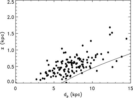
Plot for galactic bulge objects from Z95 of absolute value of z-distance versus projected distance dp (see the footnote to Table 12) based on d from Z95-Tb. The solid curve indicates how observational selection based on surface brightness in the presence of extinction might sculpt a lower envelope on the distribution.
8 SUMMARY AND DISCUSSION
8.1 Comparing distance scales: some general conclusions
Although our primary subject in this paper is construction of a system of distances for planetary nebulae, we have considered the more general problem of comparing one distance scale to another, ‘standard’ set of distances, both when the standard distances are based on trigonometric parallaxes but also when the distances have a normal or lognormal error pdf. Hence, our findings may be of broader interest.
In the former case, it is best to multiply the distances being tested by the respective parallaxes. The alternative, converting the parallaxes to distances and then dividing those by the distances to be tested, yields a biased estimate. If possible one ought to avoid discarding negative parallaxes or imprecise ones; by not discarding one completely eliminates truncation bias. Transformation bias is avoided by not converting parallax to distance. If weights are used based on the estimated errors |$\sigma ^\prime _{\cal R}$| in the distance ratio, there is likely to be a weighting bias of the sort discussed by Smith (2006). Yet if weights which depend solely on the estimated parallax error |$\sigma _\pi ^\prime$| are employed the estimate may not be efficient, since the parallax error is just one contributing factor to the error in the distance ratio and will only be dominant if λ is substantially larger than α, the relative error in the test distances; see equation (6).
In the latter case above (of a normal or lognormal error pdf for the standard distances), we find that Phillips's κ (Ph02) and Γ* (Ph04), respectively, can be useful for estimating the distance ratio, being superior to the mean of the individual distance ratios, which yields a biased and less precise estimate of the overall ratio. On the other hand, the Phillips estimators are potentially subject to domination by one or two extremely large values, as noted in Ph04. Also, in cases where the test distances have an error pdf which differs in form from that of the standard distances there can be bias; which of the two Phillips estimators is preferable depends on the parameters – typical relative errors and/or typical logarithmic errors – of the situation. Domination by a few large values, especially acute for κ, can be mitigated by using our proposed estimator ζ instead, at the cost of introducing a (usually) modest weighting bias.
When κ and ζ differ substantially without domination by an outlier, one can sometimes infer the presence of distance-dependent systematic error in one (or both) of the scales compared. The latter estimator is more nearly unaffected, although it can have weighting bias.
8.2 Calibration and testing of distance scales for planetary nebulae
Because trigonometric parallaxes are independent of astrophysical models and (in principle, at least) free of systematic error, they are a logical choice for serving as the basis for a system of distances. Other distance methods can then be tested using those parallaxes, either directly or indirectly, by using an intermediary distance scale. Some care is needed in using parallax data to avoid introducing bias. For our anchor strategy to work, the trigonometric parallaxes must be as free as possible of intrinsic systematic error. We omitted the Hipparcos ones from our calibration because they are not, in addition to being rather imprecise. One potential complication with testing is a distance dependence in the intermediary scale used or the one being tested. Another complication arises because distance methods for planetary nebulae can have radius-dependent systematic error and different samples can have different radius distributions. Here, we have shown several ways that radius dependence can arise in the calibration of a statistical scale. Indirect comparison ties the C99 spectroscopic parallaxes (but not the P96 ones) to the USNO trigonometric ones over the range in R where the two overlap, and Tb–R slopes for the two are reasonably consistent. Similarly, overlap in R ties the Magellanic Cloud Tb–R relation to the one based on H07 and C99. The unified relation is mostly consistent with those of F08 and F14, which are nearly identical to each other; a possible exception is for R > 1 pc where the latter seem underestimated. The F14 results (and ours) resolve the issue of ‘short’ versus ‘long’ statistical scales more nearly in favour of the former.
As part of the construction of a system of distances, we looked at several additional methods for which we found a few sizeable homogeneous data sets: gravity, expansion and extinction. As others have noted (e.g. B09), the N01 gravity scale seems to be too long for nearby objects (although we think it underestimates larger distances); gravity distances generally seem to have this problem, probably by underestimating g, with the possible exception of the heterogeneous sample in P96. Expansion distances need correction using astrophysical modelling (cf. F14 for an example) but can yield usable results. Extinction distances are highly problematic. Distances for one moderately large set were underestimated by almost a factor of 2. Individual distance estimates can be close but mostly are not: correlation coefficients are generally near zero. The interstellar Na D absorption distances appear to be an exception, with overestimation of perhaps only 20 per cent and r ≅ 0.7–0.8.
Comparison of the VL07 parallaxes with our ‘best estimate’ distances in the USNO system confirms the H07 preliminary finding of a systematic error in the parallaxes of approximately a factor of 2.5 for the large nebulae. There is no large overestimation in the Hipparcos parallaxes generally according to van Leeuwen's (2007b) validation study; therefore, the cause must be something intrinsic to these particular objects. Two distinguishing features are (1) the presence of nebulosity and (2) the relative faintness of the central stars – as is well-known planetary nebulae are often brighter than their central stars. We speculate that the nebulosity's parallactic shift in some subtle way affects the measurements for star images in the vicinity. One can argue that especially for the large-φ objects the surface brightness is quite low, too low for them to show up. However, what was measured by Hipparcos was photon counts, not images as such, and as far as we can tell the validation study considered only stars, not extended sources. While the contribution by that portion of a large nebula within the detector field at a given instant may be slight, the effects on a number of stars in the nebula's vicinity might add up to a significant systematic effect on the nebula's parallax, through correlated errors. It is quite clear from A98 (Section 3.1) that the nebulosity affected the parallax measurements for the small objects, not systematically but randomly, leading to noticeably larger uncertainties than for other stars of similar brightness; this is also true of the VL07 parallaxes for those same ones. For the five planetaries that are neither small nor large – He 1-5, He 2-36, NGC 40, NGC 2346 and NGC 2392 – the median is actually negative, −0.55. In fact, three of the four negative VL07 parallaxes belong to this group. The angular diameters of the three according to A98 are 10, 36 and 55 arcsec, to be compared to the 38-arcsec Hipparcos field. (The fourth is one of the smallest nebulae.) The factor of 2.5 is decidedly odd, however.
If our speculation about the effect of nebulosity on parallaxes obtained with the Hipparcos technique is correct, it has implications for other similar situations. For example, we note that Melis et al. (2014) have very recently claimed that the Hipparcos parallaxes for the Pleiades are overestimated by about 10 per cent based on very long baseline radio interferometry. If so, that overestimation might be similar to what we have found with the nebulae but less severe, possibly arising because of the reflection nebulosity in the cluster. Perhaps, the effect is much smaller because the relative brightness of the stars is greater.
8.3 Some suggestions for future work
First and foremost, there is a need for more high-precision trigonometric parallaxes. In particular, this is important for extending our type of analysis to the different categories of planetary nebulae and the specialized Sα–R relations presented in F14. It may seem as if this need will be more than satisfied by Gaia. However, according to the principles laid out herein, the Gaia parallaxes for the nebulae should be tested against HST and CCD parallaxes to make certain the former are on the USNO system. Considering the high precision of the former, a larger test sample is highly desirable. Thus far, all the accurate parallaxes we have are for objects with δ > −21°; the southern sky is practically untouched. As we already noted, almost all the H07 objects that are true planetaries have large φ; one might wish to consider especially such objects at galactic latitudes greater than 20° in absolute value as being likely to be nearby.
Secondly, the gravity method needs to be refined; empirical corrections can be used, but it is preferable to understand why it overestimates distance, at least for the nearest nebulae, and remedy the problem or at least mitigate it. Asteroseismology can be a useful testing tool as well as a means of obtaining accurate g's for getting distances, but it is model dependent and therefore must itself be checked.
Thirdly, the expansion method might benefit from switching to a different wavelength region, using the Atacama Large Millimeter/Submillimeter Array (ALMA) to observe structure in the outer nearly neutral regions of the nebulae. A digital counterpart of the Griffin ‘mask’ technique (Griffin 1967) for radial velocity measurement using multiple molecular lines originating from a given structure in the nebula might facilitate precise velocity measurement. ALMA has extensive coverage of both northern and southern sky. Of course, this might necessitate further detailed modelling along the lines of M04 and S05 to establish the expansion of the photodissociation or photon-dominated region on the outside.
Fourthly, more companions of central stars are being found (De Marco et al. 2013) and hence more spectroscopic parallaxes may be forthcoming. This approach would benefit from a uniform reduction of all the available data using a single well-calibrated set of colour-absolute magnitude relations or, failing that, several cross-correlated ones. It is highly desirable to tie that calibration to the USNO system.
When the extinction model used in G11 has been improved that method can be tested again. Perhaps different approaches to extracting a distance from the extinction curve can be tried to find one that works better than the one in G11.
We believe the problem of calibrating a statistical distance scale will not be ripe for further efforts until significant progress has been made on the foregoing, especially the first. The F14 scale is probably the best statistical one we now have, though perhaps needing some slight modification at large R.
The author has made liberal use of the SIMBAD data base and VizieR catalogue access tool operated by CDS at Strasbourg, France, and the ADS query system provided by the Smithsonian Astrophysical Observatory and NASA in this research. The original description of the VizieR service was published in A&AS, 143, 23. Thanks to Drs R. Ciardullo, H. Harris, Q. Parker, F. van Leeuwen, R. Napiwotzki, D. Frew, J. Phillips and S. Pottasch for helpful comments and criticisms and especially to Dr Frew for providing a copy of his thesis and a preprint of his 2014 paper and also to Dr A. Hajian for granting his permission to use the Hajian–Frew results. The author is also very grateful to two anonymous referees for a number of constructive criticisms and suggested improvements. Blame for any faults is of course the author's alone.
REFERENCES
APPENDIX A:
The quantities in this paper involved with distance estimation are sometimes represented by symbols that are not as familiar as the astrophysical ones. Following is a list of those used in this paper along with the page number of first appearance (for context) and equation number (if any).
B : overall distance ratio for a scale [4]
dS : true distance d multiplied by scale factor B for scale S [4]
|$d_{\rm S}^\prime$| : estimated distance in scale S [4]
F : correction factor for expansion distance; ratio true to expansion distance [19; equations (12a), (12b), (13)]
|${\cal P}_{\rm H}$| : ratio of Hipparcos parallax of an object to ‘best estimate’ parallax [21]
|${\cal R}_{\rm S}$| : distance ratio for an object in distance scale S relative to a standard distance [4]
α : relative error in a distance estimate in general [4] (Note: this departs from notation used in SE96, where α was the true relative parallax error σπ/π.)
αS : relative error for distance scale S, assumed same for all objects [5]
|$\alpha _{\rm S}^\prime$| : estimate of αS from observations [8; equations (5), (8)]
Γ : Phillips estimator for logarithm of sample distance ratio [10; equation (7)]
Γ* : dex(Γ) to give sample distance ratio [10]
κ : Phillips estimator for distance ratio [5; equation (2)]
λ : relative parallax error |$\sigma _\pi ^\prime /\pi ^\prime$| [2]
π : true trigonometric parallax of object [2]
π′ : measured trigonometric parallax of object [2]
σS : standard error of dS [4]
|$\sigma _{\rm S}^\prime$| : estimate of σS [4]
σπ : true standard error of π [2]
|$\sigma _\pi ^\prime$| : estimate of σπ [2]
|$\sigma _{\cal R}$| : standard error of |${\cal R}_{\rm S}$| [4; equation (1)]
|$\sigma _{\cal R}^\prime$| : estimate of |$\sigma _{\cal R}$| [4; equation (1a)]
ζ : modification of Phillips estimator κ to mitigate excessive weight on large distances [5; equation (3)].
