


Abstract
We present a photometric study of the globular cluster (GC) system associated with the lenticular galaxy (S0) NGC 6861, which is located in a relatively low density environment. It is based on Gemini/GMOS images in the filters g′, r′, i′ of three fields, obtained under good seeing conditions. Analysing the colour–magnitude and colour–colour diagrams, we find a large number of GC candidates, which extend out to 100 kpc, and we estimate a total population of 3000 ± 300 GCs. Besides the well-known blue and red subpopulations, the colour distribution shows signs of the possible existence of a third subpopulation with intermediate colours. This could be interpreted as evidence of a past interaction or fusion event. Other signs of interactions presented by the galaxy are the non-concentric isophotes and the asymmetric spatial distribution of GC candidates with colours (g′ − i′)0 > 1.16. As observed in other galaxies, the red GCs show a steeper radial distribution than the blue GCs. In addition, the spatial distribution of these candidates exhibits strong signs of elongation. This feature is also detected in the intermediate subpopulation. On the other hand, the blue candidates show an excellent agreement with the X-ray surface brightness profile, outside 10 kpc. They also show a colour–luminosity relation (blue tilt), similar to that observed in other galaxies. A new distance modulus has been estimated through the blue subpopulation, which is in good agreement with the previous value obtained through the surface brightness fluctuation method. The specific frequency of NGC 6861 (SN = 10.6 ± 2.1) is probably one of the highest values obtained for an S0 galaxy so far.
1 INTRODUCTION
It is known that globular clusters (GCs) are usually ancient stellar systems, with ages that can be established within a reliable and tight scale (e.g. Salaris & Weiss 2002; Mendel, Proctor & Forbes 2007) that make them good tracers of the early evolutionary stages of their host galaxies. From the observational point of view, GC systems reveal, to a greater or lesser extent, a bimodal colour distribution reaching, in some cases, a trimodal one (e.g. Blom, Spitler & Forbes 2012; Caso et al. 2013). This multimodality indicates the presence of, at least, two subpopulations of GCs, usually referred to as ‘blue’ and ‘red’ (e.g. Gebhardt & Kissler-Patig 1999; Kundu & Whitmore 2001; Larsen et al. 2001). They display different characteristics in terms of metallicity and projected spatial distribution, being the red GCs more metallic (Schuberth et al. 2010; Usher et al. 2012) and more concentrated towards their host galaxies than the blue ones.
These differences suggest that both subpopulations arose through two different processes or in two phases. Among the most cited scenarios about the origin and evolution of GC systems and their host galaxies, we find (i) the major merger formation scenario (Ashman & Zepf 1992) which proposes that the merger of two spiral galaxies (S) leads to an elliptical galaxy (E) with ‘blue’ GC donated by the spirals and the ‘red’ clusters formed in the merger; (ii) the multiphase collapse scenario (Forbes, Brodie & Grillmair 1997) which suggests that the ‘blue’ GCs are formed first and their formation is truncated by the cosmic reionization (Cen 2001), while the ‘red’ GCs and the host galaxy field stars are formed later, in a second phase; (iii) the accretion scenario (Côté, Marzke & West 1998), in which ‘red’ GCs are formed in a massive seed galaxy and the ‘blue’ GCs are accreted from satellite galaxies of lower mass. The inclusion of these scenarios in a proper cosmological framework (Beasley et al. 2002; Pipino, Puzia & Matteucci 2007; Muratov & Gnedin 2010; Tonini 2013) has shown different degrees of success and failure in explaining the observed properties of GC systems. Therefore, it is reasonable to assume that the formation process of GC systems may include ingredients from all of them.
This close relationship between the galaxies and their associated GC systems allows us to compare the predictions of different galaxy formation models with observational data. In this regard, we focus on the study of early-type galaxies and, in particular, of lenticular galaxies (S0) located in relatively low density environments. Most of the theories proposed for the origin of S0s are based on the results of different dynamical processes on normal spiral galaxies (Spitzer & Baade 1951), such as interaction with the intracluster medium (Cowie & Songalia 1977), ram-pressure stripping (Bekki, Couch & Shioya 2002; Sun et al. 2006), galactic harassment (Moore et al. 1996), etc. The presence of S0 galaxies in low-density environments can hardly be explained just by these mechanisms. Therefore, they represent a challenge to our understanding of galaxy formation and evolution.
In the last decade, GCs were used to test the formation mechanism of S0 galaxies in a few works (Aragón-Salamanca, Bedregal & Merrifield 2006; Barr et al. 2007). However, up to date, the number of lenticular galaxies with GC systems studied in detail remains relatively low. Therefore, in order to draw more firm conclusions, it is necessary to enlarge the sample of S0 GC systems deeply analysed. With that aim, we started a study which is focused on several lenticular galaxies belonging to the field or low-density groups.
In this context, we present here, as a first step, a study of the photometric properties of the GC system of the S0 galaxy NGC 6861 (Table 1). This galaxy is located in the Telescopium group (AS0851) at a distance of 28.1 Mpc (Tonry et al. 2001), and is one of the brightest galaxies in the group together with the E galaxy NGC 6868. Chandra observations show that NGC 6861 might be undergoing an interaction with NGC 6868, suggesting the fusion of two subgroups (Machacek et al. 2010). NGC 6861 presents an unusually high central stellar velocity dispersion of ∼414 km s−1 (Wegner et al. 2003), and from that Machacek et al. (2010) inferred the presence of a supermassive black hole. Recently, Rusli et al. (2013) included this galaxy in their sample of 10 massive early-type galaxies. They found that NGC 6861 (along with NGC 4751, another S0 galaxy) shows the fastest rotation and the highest dispersion in their sample and confirmed the high dynamical mass for this black hole (see Table 1).
Galaxy properties. Columns (2)–(5) show equatorial and galactic coordinates (NED); (6) morphological classification (NED); (7) B magnitude from the RC3 catalogue (de Vaucouleurs et al. 1991); (8) distance modulus from Tonry et al. (2001); (9) effective radius from RC3; (10) central velocity dispersion calculated into a circular aperture of radius r = 0.595 h−1 kpc (Wegner et al. 2003); (11) velocity dispersion within Re and (12) black hole mass from Rusli et al. (2013).
| Galaxy | αJ2000 | δJ2000 | l | b | Type | |$B_{T}^{ 0}$| | (m − M)0 | Re | σ0 | σe | MBH |
|---|---|---|---|---|---|---|---|---|---|---|---|
| (h:m:s) | (° : ′ : ′′) | (° : ′ : ′′) | (° : ′ : ′′) | (mag) | (mag) | (arcsec) | (km s−1) | (km s−1) | (M⊙) | ||
| NGC 6861 | 20 : 07 : 19.5 | −48 : 22 : 13 | 350 : 52 : 38 | −32 : 12 : 39 | SA(s)0− | 11.92 | 32.24 | 17.7 | 414±17 | 388.8±2.6 | 2.2(2.1, 2.4) × 109 |
Observations of NGC 6861, comparison field and blank sky. The values of airmass, exposure time and FWHM correspond to the final co-added images. Field 1 contains the galaxy.
| Galaxy | Field | Airmass | Texp | FWHM |
|---|---|---|---|---|
| (s) | (arcsec) | |||
| g′ r′ i′ | g′ r′ i′ | g′ r′ i′ | ||
| NGC 6861 | 1 | 1.053 1.056 1.067 | 4×700 4×350 4×400 | 0.88 0.75 0.82 |
| 2 | 1.342 1.251 1.181 | 4×700 4×350 4×400 | 0.62 0.48 0.43 | |
| 3 | 1.272 1.095 1.134 | 4×700 4×350 4×400 | 0.57 0.80 0.77 | |
| Comp. field | – | 1.026 1.022 1.039 | 14×180 14×120 17×90 | 0.56 0.58 0.53 |
| Blank sky | – | – – 1.107 | – – 7×300 | – – – |
The GC system of NGC 6861 was previously studied by Kundu & Whitmore (2001). They analysed the GC systems of 29 S0 galaxies in the V and I bands (one image of 160 s in the F555W filter and two images of 160 s in the F814LP filter), observed between 1995 September 6 and 1996 May 3 with the Wide Field Planetary Camera 2 (WFPC2) of the Hubble Space Telescope. That work raises the possibility of the existence of bimodality in the colour distribution of the GC candidates in the range 0.5 < V − I < 1.5 mag. Besides, the authors estimated a total GC population in their WFPC2 field of 1858 GCs and a corresponding local specific frequency of SN = 3.6 ± 1.6.
2 DATA
2.1 Observations and data reduction
We worked with images obtained in 2010 July–November, using the Gemini Multi-Object Spectrograph (GMOS; Hook et al. 2004) of Gemini-South (Cerro Pachon, Chile) in imaging mode. The instrument consists of three 2048 × 4608 pixel CCDs, separated by two ∼2.8 arcsec (39 pixel) gaps, with a scale of 0.0727 arcsec pixel−1. The field of view (FOV) of the GMOS camera is ∼5.5 × 5.5 arcmin. Our images were taken under photometric conditions and using a 2 × 2 binning, which gives a scale of 0.146 arcsec pixel−1 (programme GS-2010B-Q-2, PI: Bassino). Three deep fields were observed in the g′, r′ and i′ filters (Fukugita et al. 1996), similar to those of the Sloan Digital Sky Survey (SDSS). The seeing conditions were excellent, ranging from 0.43 to 0.88 arcsec. As can be seen in Fig. 1, one of the fields was centred in NGC 6861. In order to fill in the gaps and facilitate removal of cosmic rays and bad pixels, four slightly dithered exposures were taken per filter.
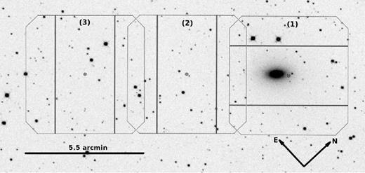
SDSS image with the three superimposed GMOS fields.
The raw data were processed by using Gemini-GMOS routines within iraf1 (e.g. GPREPARE, GBIAS, GIFLAT, GIREDUCE and GMOSAIC), and applying the appropriate bias and flat-field corrections. The bias and flat-field images were acquired from the Gemini Science Archive (GSA) as part of the standard GMOS baseline calibrations.
It is known that i′ and z′ frames taken with GMOS show night-sky fringing. To subtract this pattern from our i′ data, it was necessary to create fringe calibration images by using the task GIFRINGE. These frames were built from seven i′ blank sky images taken with exposure times of 300 s. Subsequently, the night-sky fringing was removed from our i′ images using the task GIRMFRINGE.
As a final step, the reduced images corresponding to the same filter were co-added using the task IMCOADD, obtaining g′, r′ and i′ co-added images for each field. These final images (see Table 2) were then used for the subsequent photometric analysis.
2.2 Photometry and classification of unresolved sources
The source detection was performed on the g′ images because they present a better signal-to-noise ratio than the r′ and i′ frames. In order to do that, we used a script that combines features of SExtractor (Bertin & Arnouts 1996), along with iraf filtering tasks. It allows us to model and subtract both the background and the brightness due to the galaxy halo. To do this, initially, stellar objects were removed by using SExtractor, and then the residual image was smoothed with a median filter, employing the FMEDIAN task from iraf. This median filtered image was then subtracted from the original image. The procedure was applied a second time on the last image using a smaller median filter to detect and to discard weak haloes around objects near the galactic centre (Faifer et al. 2011). For each field, the script provides a final catalogue with all detected objects and a galaxy light subtracted image.
From these lists of objects, ∼50 bright unresolved sources were selected per field, uniformly distributed over the FOV. Then, second-order models of the point spread function (PSF) were obtained using the daophot package (Stetson 1987) within iraf. Several tests were performed with different PSF models, selecting the Moffat25 model, which gives lower fit errors than the Gaussian and Moffat15 options. The same procedure was applied to the r′ and i′ images of the same field. In order to obtain the instrumental PSF magnitudes of all the detected sources, we applied the ALLSTAR task on each image, using their respective PSF models and the object list of the reference filter (g′). In addition, we conducted an aperture correction to the PSF magnitudes through the MKAPFILE task. As a final step, we built a master photometric catalogue in which the coordinates of objects belonging to different fields were in the same reference system. To do this, we selected common sources located in the overlapping regions of the fields and worked with the tasks GEOMAP and GEOXYTRAN within iraf.
At the distance of NGC 6861, we expect that GC candidates are unresolved sources. Therefore, the stellarity index of SExtractor (0 for resolved objects and 1 for unresolved ones) was used to make the object classification. We set resolved/unresolved boundary in 0.5.
2.3 Photometric calibration
Several standard star fields observed during the same nights as our frames were downloaded from the GSA data base (see Table 3). All of them are from the list of ‘Southern Standard Stars for the u′ g′ r′ i′ z′ System’ of Smith et al. (in preparation).2 Exposure times for these images were 5.5 s for the g′, r′ and 4.5 s for the i′ filter. They were reduced using the same bias and flat-field images previously used for the reduction (see Section 2.1).
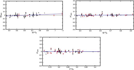
Residual zero-points as a function of the standard colour index. Red, grey and black circles represent the photometric measurements performed on standard stars in the fields mentioned in Table 3. The blue line shows the obtained fit.
Standard fields used for the photometric calibrations. *S: number of standard stars in the field. KCP: atmospheric extinction coefficient at Cerro Pachon. m|$_{{\rm zero}}^{*}$|: zero-point obtained from the fit.
| Standard field | *S | Science field | Filter | KCP | m|$_{{\rm zero}}^{*}$| |
|---|---|---|---|---|---|
| 020000_300600 | 2 | 1 | g′ | 0.18 | 28.42±0.010 |
| 220100_300000 F1 | 4 | ||||
| 180000_600000 | 15 | r′ | 0.10 | 28.33±0.003 | |
| 180000_600000 F5 | 16 | ||||
| E8_a F1 | 12 | ||||
| 180000_600000 | 15 | i′ | 0.08 | 27.92±0.004 | |
| 180000_600000 F5 | 16 | ||||
| E8_a F1 | 12 | ||||
| 180000_600000 | 15 | 2 | g′ | 0.18 | 28.41±0.006 |
| 180000_600000 F5 | 16 | ||||
| 220000_595900 F1 | 4 | ||||
| 180000_600000 | 15 | r′ | 0.10 | 28.44±0.004 | |
| 180000_600000 F5 | 16 | ||||
| 220000_595900 F1 | 4 | ||||
| 180000_600000 | 15 | i′ | 0.08 | 28.01±0.006 | |
| 180000_600000 F5 | 16 | ||||
| 220000_595900 F1 | 4 | ||||
| 020020_600000 | 4 | 3 | g′ | 0.18 | 28.24±0.016 |
| CDFS | 2 | ||||
| 020020_600000 | 4 | r′ | 0.10 | 28.30±0.011 | |
| CDFS | 2 | ||||
| 020020_600000 | 4 | i′ | 0.08 | 27.92±0.005 | |
| CDFS | 2 |
Residual zero-point, colour terms and the final photometric zero-points for field 2, obtained with the linear fits.
| Filter | a | CT | (m1 − m2) | mzero |
|---|---|---|---|---|
| g′ | −0.054±0.019 | 0.08±0.03 | (g′ − r′) | 28.36±0.02 |
| r′ | −0.018±0.011 | 0.03±0.01 | (g′ − r′) | 28.42±0.01 |
| i′ | 0.006±0.013 | −0.02±0.05 | (r′ − i′) | 28.01±0.01 |
| Filter | a | CT | (m1 − m2) | mzero |
|---|---|---|---|---|
| g′ | −0.054±0.019 | 0.08±0.03 | (g′ − r′) | 28.36±0.02 |
| r′ | −0.018±0.011 | 0.03±0.01 | (g′ − r′) | 28.42±0.01 |
| i′ | 0.006±0.013 | −0.02±0.05 | (r′ − i′) | 28.01±0.01 |
Finally, objects in common in each science field were used to obtain any small zero-point differences between our field 2 and the other pointings, resulting in values lower than 0.03 mag in all cases. These small offsets were applied in order to refer our photometry to field 2. Subsequently, we visually rejected spurious detections and artefacts from our master catalogue (less than 1 per cent of total sources) and applied the Galactic extinction coefficients, given by Schlafly & Finkbeiner (2011) (Ag = 0.179, Ar = 0.124, Ai = 0.092).
2.4 Completeness test
To quantify a reliable detection limit of unresolved objects in our photometry, we performed a series of completeness tests in each filter and each field. We split the range 20.1 < |$g^{\prime }_0$| < 29.5 mag into intervals of 0.2 mag, adding 200 point sources using the ADDSTAR task. A total number of 9600 artificial objects were added in each field. The spatial distribution of the artificial objects was carried out using a power law, trying to follow the radial distribution of the GC candidates. Subsequently, the same script mentioned in Section 2.2 was applied to these images, in order to recover the added objects.
Fig. 3 shows the completeness curves for the three fields, plotting the fraction of artificial objects recovered versus the input magnitude. It can be seen that, at |$g_0^{\prime }$| = 25.5 mag, the data have a completeness greater than 80 per cent. Thus, in the following analysis, we will take a faint cut magnitude of |$g_0^{\prime }=25.5$| mag. Fig. 4 shows the completeness fraction for different ranges of magnitudes as a function of galactocentric radius (Rgal). It can be seen that most of the objects are lost at small Rgal, due to the high brightness of the galaxy. Taking this completeness variation into account, we can conclude that for magnitudes brighter than |$g_0^{\prime }$| = 25.5, we detect the vast majority of GCs over the whole NGC 6861 field, except in the inner 30 arcsec of Rgal (1.7Re) where most of the objects are lost.
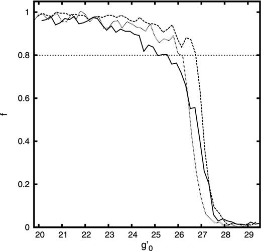
Completeness fraction as a function of |$g^{\prime }_0$| magnitude. The solid, dashed and dotted lines correspond to fields 1, 2 and 3, respectively. The horizontal dotted line shows the 80 per cent completeness level.
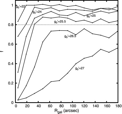
Completeness fraction as a function of galactocentric radius for field 1. The curves (from top to bottom) show the completeness for |$g^{\prime }_0$| = 22, 24, 25, 25.5, 26.5, 27 mag. The horizontal dashed line shows the 80 per cent completeness level.
2.5 Comparison field
We were not able to get a comparison field as part of our Gemini programme and, as we will mention in Section 3.5, our GC candidates seem to fill the whole field. Therefore, in order to estimate the background contamination, we had to search for deep g′, r′ and i′ fields in the GSA. We found only one nearby GMOS frame which filled our requirements. This field, centred in the compact galaxy group NGC 6845 (RA = |$\mathrm{20^h00^m58{^{\rm s}_{.}}28}$|, Dec. = |$\mathrm{-47^d04^m11{^{\rm s}_{.}}9}$|), is part of the Gemini programme GS-2011A-Q-81 (PI: Gimeno). We downloaded the raw images and reduced and calibrated them according to the procedure explained in Sections 2.1 to 2.4.
Unresolved objects were selected using the same ranges in colour and magnitude of our GC candidates in NGC 6861 (see Section 3.2). In Fig. 5, we show the colour–magnitude diagram (CMD) for the unresolved sources obtained for this field. The completeness test on the g′ frame shows that we have a completeness >80 per cent for g′ < 26 mag. After that value, the completeness falls down strongly and colour errors grow rapidly.
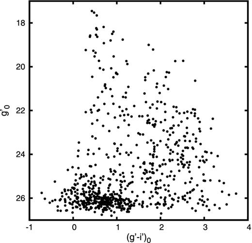
CMD of the point sources detected in the NGC 6845 field.
It is important to mention that the NGC 6845 group is composed of four galaxies. All of them are well contained inside the GMOS FOV. Two of these galaxies are spirals and two are of S0 type. The only available estimation of the distance to the group is based on the galaxy redshifts and they give values from 90 to 100 Mpc (Gordon, Koribalski & Jones 2003). Adopting this range of distances and the V-to-g′ band relation from Faifer et al. (2011), we can expect that massive GCs like ω Cent will show |$g^{\prime }_0\sim 24.8\hbox{--}25.1$| mag. Then, as a first step we should check if the GCs belonging to these galaxies are detected in our photometry. The CMD shown in Fig. 5 indicates that no particular grouping is detected for objects in the colour ranges typical of GCs. We performed the same test using the colour–colour diagrams and the results were similar. As an additional test we made plots of the spatial distribution of the point sources and only those objects with |$g^{\prime }_0$| > 24.5 mag seem to show some very marginal concentration towards the galaxies. Therefore, as expected from the assumed distance, some of the fainter objects in NGC 6845 may well be GCs belonging to the galaxies in the group.
We excluded the zones near the four galaxies and we applied the same magnitude cuts as in the NGC 6861 sample (see Section 3.2) and thus only 36 point sources survive in the NGC 6845 field (Fig. 6). This is a very low number and if we accept that some of them could be GCs belonging to the group, it means that our NGC 6861 photometry has a contamination lower than 8 per cent. In what follows, we will take these 36 objects as our contamination estimation.
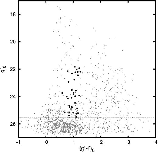
CMD of the point sources in the comparison field. Black filled circles show colours and magnitudes inside the ranges adopted for the GC candidates in NGC 6861.
3 RESULTS
3.1 Galaxy surface profile and tidal structures
We obtained the surface brightness profile of NGC 6861 using the iraf task ELLIPSE which fits elliptical isophotes to the galaxy. In order to avoid the light contribution from nearby bright or extended objects, before executing ELLIPSE we masked them in the image. We modelled the galaxy light allowing the centre, ellipticity and position angle (PA) of the isophotes to vary freely until the fit became unstable in the outer regions. It is important to remember that the GMOS FOV is small and NGC 6861 fills it completely. Therefore, all the parameters mentioned here are limited to Rgal < 2 arcmin.
The results are shown in Fig. 7. It can be seen that the ellipticity undergoes strong variations from 0.46 to 0.2 within 100 arcsec, whereas the PA shows a difference of ∼44 between the innermost zone and the radius mentioned above. This ellipticity decrement is also seen in the X-ray hot gas emission from e = 0.4 ± 0.04 to 0.19 ± 0.05 for 7.3 ≤ r ≤ 42 kpc (Machacek et al. 2010).
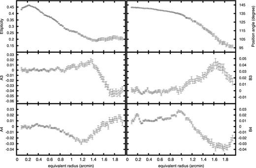
Isophotal parameters for the g′ filter versus equivalent galactocentric radius. The latter was calculated as the square root of the product of the semi-major and semi-minor axis lengths of the fitted ellipses. From left to right and from top to bottom, the graphics show the ellipticity and PA of the isophotes, and the Fourier coefficients A3, B3, A4, B4, respectively.
These changes in the isophotal parameters are also detected in the Fourier terms (A3, B3, A4, B4), which measure the isophote's deviations from perfect ellipticity. The terms A3 and B3 give ‘egg-shaped’ or ‘heart-shaped’ isophotes, but the most significant term is the coefficient B4 (Jedrzejewski 1987). According to its sign, E/S0 galaxies can be classified into discy (B4 > 0) or boxy (B4 < 0). In our case, within 1 arcmin, B4 indicates discy isophotes. At larger radii, the parameter B4 changes its sign showing that NGC 6861 displays boxy isophotes. These results are in agreement with those obtained by Li et al. (2011) in the the Carnegie-Irvine Galaxy Survey. It is interesting to mention that boxy isophotes are usually suggestive of recent merging (Kormendy & Bender 1996).
The variation shown by the PA in NGC 6861 was previously reported by Tal et al. (2009). These authors mentioned that this galaxy has tidal characteristics, showing intra-group emission and non-spherical isophotes. Therefore, we searched for this kind of evidence in our deep GMOS images. In the left-hand panel of Fig. 8, we show the r′ image of NGC 6861. It can be seen that the galaxy isophotes are not concentric, showing a deformation towards the NW. The right-hand panel in that figure shows the ratio between the original r′ image and the smooth ellipse model. Several distinct structures are evident in NGC 6861, starting by a dust and stellar disc labelled with ‘A’ (Rgal < 10 arcsec), a series of more external arcs (where the brightest are labelled with ‘B’ and ‘C’), and two diffuse stellar debris or low surface brightness structures. The feature located in the NW was labelled with ‘D’ and that in the SE with ‘E’. Unfortunately, ‘D’ presents a bright star on it. Between ‘C’ and ‘D’ there is clearly another structure. The structure ‘E’, which is not symmetrically located with respect to ‘D’, is easily visible and shows a sharp external edge. All of them lie along the inner major axis of the galaxy.
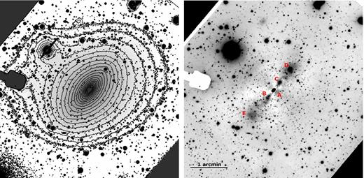
Left: r′ isophotes of NGC 6861 (field 1). The faintest and more external isophote corresponds to |$\mu _{r^{\prime }}$| = 24.5 mag arcsec−2, and brightest and inner to |$\mu _{r^{\prime }}$| = 17.5 mag arcsec−2. The steps between them are 0.368 mag arcsec−2. Right: ratio between the original r′ image and the model. It is possible to see the different structures present inside of NGC 6861. The most obvious and easily visible structures were labelled by letters ‘A’ to ‘E’. North is up and east is to the left.
Finally, and in order to compare the spatial light distribution of NGC 6861 with that of the GCs, we obtained a more extended surface brightness profile for the galaxy. Although the images of fields 1 and 2 were taken on different days, Table 4 shows that the photometric conditions were similar. Therefore, we followed the same procedures as those included in the task IMCOADD, used the overlapping area of fields 1 and 2 to equalize the signal and the sky level of the g′ images, and built a mosaic including these two fields. After checking the photometric scales by comparing common objects in the original images with those in the final mosaic, we run ELLIPSE and we get a profile reaching 6 arcmin of semi major axis (sma) (Fig. 9). The inner zone of the profile (sma < 70 arcsec), which is saturated in our long-exposure images, was obtained by running ELLIPSE on a short-exposure g′ image.
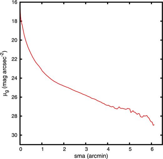
Radial surface brightness profile of NGC 6861 in filter g′.
3.2 GC colours
Fig. 10 shows the |$g^{\prime }_0$| versus (g′ − i′)0 CMD, as well as the (g′ − r′)0 versus (g′ − i′)0 and the (g′ − r′)0 versus (r′ − r′)0 colour–colour diagrams, which include all the unresolved sources detected in the three GMOS fields. As can be seen, GCs are easily identified as point sources clustered around specific colours and most of these unresolved objects define a clear sequence, which is highlighted above the sequence of the Milky Way (MW) stars. In order to obtain our sample of GC candidates, we selected the objects within the colour ranges 0.5 < (g′ − r′)0 < 0.95 mag, 0.05 < (r′ − i′)0 < 0.5 mag and 0.55 < (g′ − i′)0 < 1.45 mag. We expect that a small percentage of the GC candidates are foreground stars and possible ultra-compact dwarfs (UCDs; Drinkwater et al. 2003). To separate bright GCs from UCDs and/or field stars, we took |$g_0^{\prime }$| = 21.8 mag as the bright end in the CMD, which is roughly equivalent to MV ∼ −11 mag (in agreement with the value suggested by Mieske et al. 2006a). The adopted faint end was |$g_0^{\prime }$| = 25.5 mag, where we ensure a completeness level greater than 80 per cent, and colour photometric errors lower than 0.1 mag.
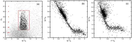
Colour–magnitude (a) and colour–colour diagrams (b,c) of all of the detected point sources in the three fields (black dots), and the initial sample of GC candidates (black filled circles). Mean photometric errors (g′ − i′)0 are shown in panel (a) by red bars. The red box shows the limits used in colour and magnitude for the selection of GC candidates.
The final sample of GC candidates for the subsequent analysis is shown in Fig. 11. A total of 1245 objects meet the above criteria. The figure shows all the candidates identified before performing any statistical subtraction of field contamination.
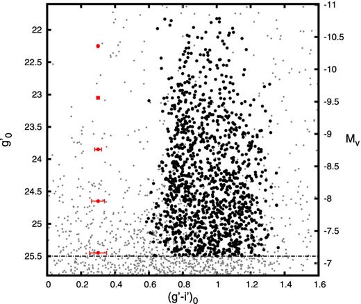
CMD of the final GC candidates (black filled circles); the dashed line shows the 80 per cent completeness level.
At first glance, the CMD seems to show bimodality, displaying a marked blue subpopulation and a more disperse, but large, red subpopulation. Interestingly, Fig. 11 shows that the blue sequence of GCs seems to become redder with increasing luminosity. This particular characteristic shown by NGC 6861 is known as ‘blue tilt’. We will discuss it in Section 3.4.
3.3 Colour histograms
Due to the large number of GC candidates, we were able to build colour histograms counting objects in small bins of 0.05 mag. In the upper panel of Fig. 12, we show the histogram obtained for all candidates in the sample and the expected contamination obtained, as was indicated in Section 2.5. A factor of 3.0 was applied to the contaminant object counts in order to take into account the different areas of the NGC 6861 and NGC 6845 fields. As was mentioned in that section, the number of MW stars and background galaxies in the GCs sample seems to be very low. Therefore, in the lower panel of Fig. 12 we show the histogram corrected by the background contamination and, as expected, the correction had a negligible effect on the integrated colour distribution. In the same figures, we show the respective smoothed colour distributions obtained using a Gaussian kernel of σ = 0.04 mag. This σ value was considered to be representative of the mean error in (g′ − i′)0 colours for fainter candidates.
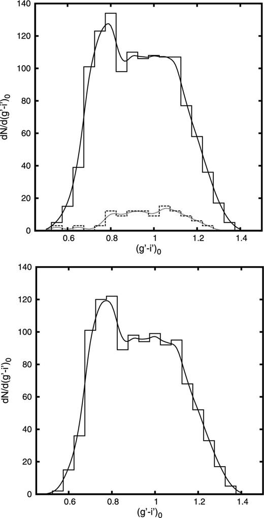
Upper panel: (g′ − i′)0 colour histograms for the GC candidates and comparison field (dashed lines) with magnitudes within 21.8 < |$g_0^{\prime }$| < 25.5. The solid and dotted lines represent the smoothed colour distributions. Bottom panel: background-corrected colour histogram and smoothed distribution.
To quantify the modes and dispersions of the different subpopulations of GC candidates, we used the statistical algorithm Gaussian mixture model (GMM; Muratov & Gnedin 2010). This method is a parametric probability density function represented as a weighted sum of Gaussian component densities. Using three statistics, which are (1) parametric bootstrap method (low values indicate a multimodal distribution), (2) separation of the peaks between Gaussians (D > 2 implies multimodal distribution) and (3) kurtosis of the input distribution (k < 0 condition necessary but not sufficient for bimodality), GMM quantifies whether a multimodal distribution provides a better fit than a unimodal one. It also allows us to define initial values for the modes and fits equal dispersions (homoscedastic) or different dispersions (heteroscedastic) to the components.
We started by fitting two Gaussian distributions and finding mean colours for the expected ‘classic’ blue and red GCs. The brightest objects (|$g^{\prime }_0$| < 22.8 mag) were rejected in order to avoid the effect of the ‘blue tilt’ and the usual unimodal colour distribution of these massive objects. The values obtained, listed in Table 5, are in good agreement with the location of the peaks found in other galaxies by Faifer et al. (2011). In that work, the authors present results for another bulge-dominated S0 galaxy, NGC 3115, which is considered now as one of the most clear examples of bimodality in colour (〈g′ − i′〉0 ∼ 0.765 ± 0.007 and 〈g′ − i′〉0 ∼ 1.044 ± 0.011 for blue and red GCs, respectively) and in metallicity (Brodie et al. 2012). Interestingly, NGC 3115 shows more or less the same luminosity as NGC 6861, but the latter presents a larger GC population and its bimodality is not as clear.
Values obtained with GMM and rmix for the (g′ − i′)0 colour distribution. Statistics values (p, D, k, χ2) are listed along with the mean colour μ, their dispersion σ and the fraction of objects assigned by rmix for each subpopulation for the bimodal and trimodal case.
| GMM | rmix | |||||||||
|---|---|---|---|---|---|---|---|---|---|---|
| Population | Bimodal case | Trimodal case | Bimodal case | Trimodal case | ||||||
| Statistics values | (p = 0.01; D = 2.63±0.14; | (p = 0.01; D = 2.46±0.34; | (χ2 = 15.639) | (χ2 = 5.869) | ||||||
| k = −0.934) | k = −0.934) | |||||||||
| μ | σ | μ | σ | μ | σ | f | μ | σ | f | |
| Blue | 0.79 ± 0.02 | 0.08 ± 0.007 | 0.783 ± 0.014 | 0.075 ± 0.009 | 0.783 ± 0.01 | 0.07 ± 0.006 | 0.376 ± 0.023 | 0.778 ± 0.02 | 0.07 ± 0.003 | 0.379 ± 0.025 |
| Green | – | – | 0.954 ± 0.062 | 0.066 ± 0.032 | – | – | – | 0.955 ± 0.03 | 0.07 ± 0.020 | 0.227 ± 0.140 |
| Red | 1.07 ± 0.02 | 0.12 ± 0.007 | 1.128 ± 0.058 | 0.10 ± 0.022 | 1.066 ± 0.014 | 0.13 ± 0.008 | 0.624 ± 0.023 | 1.136 ± 0.04 | 0.10 ± 0.016 | 0.394 ± 0.127 |
Fig. 12 shows that the red subpopulation in NGC 6861 presents a broad and flat colour distribution. Blom et al. (2012) found similar characteristics in the massive elliptical galaxy NGC 4365, where the existence of a third subpopulation of GCs with intermediate colours is proposed. In order to study whether the same situation occurs in NGC 6861, we split the sample of GC candidates into four radial bins with approximately 310 objects in each of them (Rgal ≤ 46, 46–93, 93–160 and >160 arcsec). The background-corrected colour distributions are shown in Fig. 13. A Gaussian kernel was used in order to obtain smoothed colour distributions, as described earlier. We can see that in the inner region there is a clear blue subpopulation at modal value (g′ − i′)0 ∼ 0.85. Besides this, a clearer red peak is easily detected at modal colour of (g′ − i′)0 ∼ 1.10. As we move towards outer regions, and as expected, the blue GCs begin to dominate. However, the red GC candidates become more heterogeneous and at least two other possible peaks seem to appear. One of them in (g′ − i′)0 ∼ 0.94 and the other one around (g′ − i′)0 ∼ 1.10–1.15 mag.
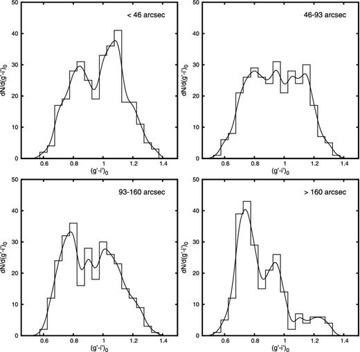
Colour distribution of the GC candidates, separated into four radial bins, according to their galactocentric distance (0–46, 46–93, 93–160 and >160 arcsec). The solid line represents the applied Gaussian kernel.
With the purpose of quantifying and characterizing the possible presence of three subpopulations, we ran GMM to the colour distribution and the rmix4 software to the histogram (whole sample background-corrected histogram), fitting in both cases a trimodal distribution. The obtained values for the GMM fit, listed in Table 5, indicate that a trimodal distribution is as good as a bimodal one. On the other hand, the reduced chi-square values obtained with rmix indicate that a trimodal case gives a better fit to the data than the bimodal one.
In different early-type galaxies, the mean colour of the red GCs was found to be similar to the inner halo colour of their host galaxies (Forbes & Forte 2001). This is the consequence of the bulge/spheroid field stars and red GCs having a strong genetic nexus (Forte, Vega & Faifer 2009). Through the task ELLIPSE, we obtained an approximate colour profile for NGC 6861 (see Section 3.1). This profile was calculated within a radius less than 2 arcmin, in order to avoid the strong effect of the error in the sky level. In the upper panel of Fig. 14, we compare the colour of the galaxy halo with the mean colour of the GCs for the bimodal case. To separate blue and red subpopulations, we consider the colour cut in (g′ − i′)0 = 0.90. It can be seen that the red GCs look similar to the inner halo, although somewhat bluer. However, considering a trimodal case [(g′ − i′)0 ≤ 0.88, 0.88 < (g′ − i′)0 < 1.01 and (g′ − i′)0 ≥1.01, for blue, green and red subpopulations, respectively], we can see that the red GCs look almost identical in colour to the halo (lower panel in Fig. 14). In both cases, the GC subpopulations were split using the values provided by GMM, and subsequently mean colours were obtained within several galactocentric intervals containing the same number of objects, 85 GCs in the bimodal case and 51 in the trimodal one. It is interesting to see that fig. 16 in Blom et al. (2012) presents similar results.
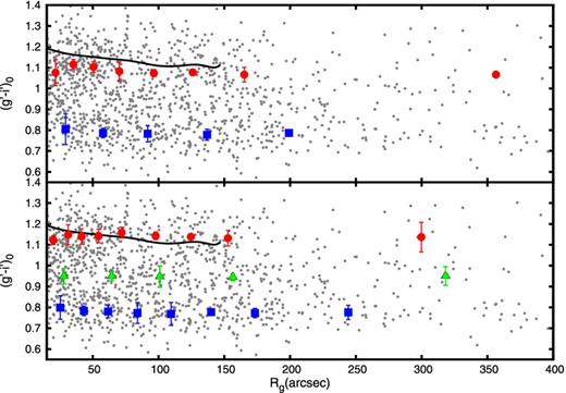
Colour index (g′ − i′)0 versus projected galactocentric radius. The bimodal case is plotted in the upper panel and the trimodal case in the bottom panel. Red circles, blue squares and green triangles represent mean values in colour for the red, blue and intermediate subpopulations, respectively. The black line shows the profile colour of the galaxy within a 2.5 arcmin radius.
3.4 Blue tilt
As mentioned in Section 3.2, the blue GC candidates of NGC 6861 seem to follow a colour–magnitude trend, known as ‘blue tilt’. A similar phenomenon was observed in several elliptical galaxies (see Forte, Faifer & Geisler 2007; Peng et al. 2008; Wehner et al. 2008; Harris 2009a). This trend has been interpreted as an increase of the metallicity with the GC mass, i.e. a mass–metallicity relation (MMR). Physics explanations for the ‘blue tilt’ were proposed by Strader & Smith (2008) and Bailin & Harris (2009), based on self-enrichment during a cluster's formation stage, where star formation is influenced by supernova feedback within the protocluster.
With the aim to characterize this MMR in NGC 6861, the sample of GC candidates was split into several magnitude bins of 100 objects. Subsequently, rmix was used to obtain the locus of peaks in each bin for the three subpopulations mentioned in Section 3.3 (GMM gave us similar results, but rmix was preferred due to its graphical direct interface). In this case, we made homoscedastic runs in order to facilitate the convergence (the three modes have the same variance) and tested with bins of different widths. In Fig. 15, we show, as an example, the mean values for blue, green and red candidates obtained considering bins of 0.075 mag in an i′ versus (g′ − i′)0 CMD. The figure shows that, as was suspected earlier from the CMD, the blue peak indeed becomes redder at higher luminosities.
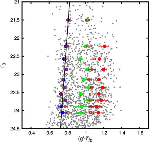
Blue tilt present in NGC 6861 (black line) for trimodal case. Blue, green and red filled circles represent peak values in (g′ − i′)0 colour obtained by rmix for blue, green and red subpopulations, respectively. The brown open squares correspond to the peak values considering the bimodal case for blue and red subpopulations.
Harris (2009a) found evidence that the blue tilt in M87 begins to be detectable from magnitudes brighter than MI = −9.5, exhibiting a non-linear behaviour. Using the equation (1) from Faifer et al. (2011) and the adopted distance to NGC 6861, we obtained the equivalent value |$i^{\prime }_0\sim 23.24$| mag. Regarding the slope of the tilt obtained by Harris, it was d(g − i)/di = −0.021 ± 0.004. However, values slightly larger than that were obtained for other galaxies. For example, Faifer et al. (2011) found d(g′ − i′)/di′ = −0.032 ± 0.003 (for luminosity MI ≤ −9.5) for the giant elliptical galaxy M 60, and Wehner et al. (2008) found d(g′ − i′)/di′ = −0.044 ± 0.011 (for luminosity MI ≤ −9) for NGC 3311.
In order to compare with the different values from the literature, we made a linear least-squares fit to the colour as a function of |$g^{\prime }_0$| and |$i^{\prime }_0$| magnitudes. We use this functional form as a first-order approach and because it is worthless to use a more complex functional form for this particular sample of points.
In order to facilitate the comparison of our results with other values present in the literature, we additionally run rmix forcing it to fit a bimodal distribution to the same sample as used in the trimodal case. In this opportunity, we made heteroscedastic runs (that means that different mode variances are allowed), and the resulting peaks of the two Gaussians for different magnitude bins are also shown in Fig. 15. We can see that the blue peak is clearly recovered, and that most of them are very close to the points obtained in the trimodal case. On the other hand, the new red peaks are located between the ‘green’ and ‘red’ candidates of the trimodal case. A linear fit to the blue peak points using the whole sample gives |$(g^{\prime }-i^{\prime })_0 = -0.021(\pm 0.011) i^{\prime }_0+1.258 (\pm 0.257)$|. When only the points brighter than |$i^{\prime }_0 = 23.3$| are included, the fit results in |$(g^{\prime }-i^{\prime })_0 = -0.033 (\pm 0.010) i^{\prime }_0+1.539(\pm 0.239)$|. Within the errors, these values are the same as those in equations (3)–(5) and very similar to those obtained for several elliptical galaxies, as mentioned before.
The adopted values for the blue tilt in the bimodal or trimodal cases do not necessary imply that the MMR is linear for NGC 6861. Our tests indicate that the slope, considering different subsamples, seems to decrease as we consider the weakest magnitude points in the CMD [as found in other galaxies like those presented by Mieske et al. (2010) and Harris (2009a)]. However, the errors associated with those estimations are too big, indicating that we probably need a more deeper sample to obtain conclusive results. For that reason, in this paper we decided to compare our results only with estimates of linear fits in the literature.
As mentioned before, the different estimates found in the literature on the blue tilt, mostly for elliptical galaxies, are similar to that obtained here. This is true even when we compare slopes from other combinations of photometric filters. For example, the results of Usher et al. (2013) for NGC 4278, or those from Mieske et al. (2006b) and Strader et al. (2006) for M49, M60 and M87, are all around d(g′ − z′)/dz ∼ −0.040. This value is equivalent to that obtained by us in NGC 6861 when we use the relation between the Advanced Camera for Surveys (ACS) (g′ − z′) and (g′ − i′) filters from Forte et al. (2013).
In a similar way as was done for blue GCs, we performed linear fits for green and red candidates in the trimodal case, obtaining d(g′ − i′)/di′ = −0.009( ± 0.022) and d(g′ − i′)/di′ = −0.019( ± 0.018), respectively. As can be seen, the slope for green GCs is not significant whereas in the case of the red GCs, a weak red tilt is obtained, though the value of this slope has a marginal significance. When we force the bimodal case and we fit the read peak, we get d(g′ − i′)/di′ = 0.012(±0.009). This slope has the opposite sign to that of the trimodal case. However, this marginally significant slope disappears when the brightest point is rejected. Therefore, we think that no slope is present in the red peak sample when bimodality is assumed.
3.5 Spatial distribution
In Fig. 16, we show the projected spatial distribution of the three subpopulations according to the separation of GMM mentioned in Section 3.3. In this figure the different spatial distributions of blue and red candidates are shown. The latter looks more concentrated and flattened, resembling the starlight distribution of NGC 6861 (see Section 3.6). On the other hand, we have obtained the radial unidimensional distributions of GC candidates. The surface density for each radial bin was obtained counting the GC candidates in annuli, and applying a factor to take into account the fraction of area effectively observed of each annulus. In every case, the associated density error is given by Poisson statistics.
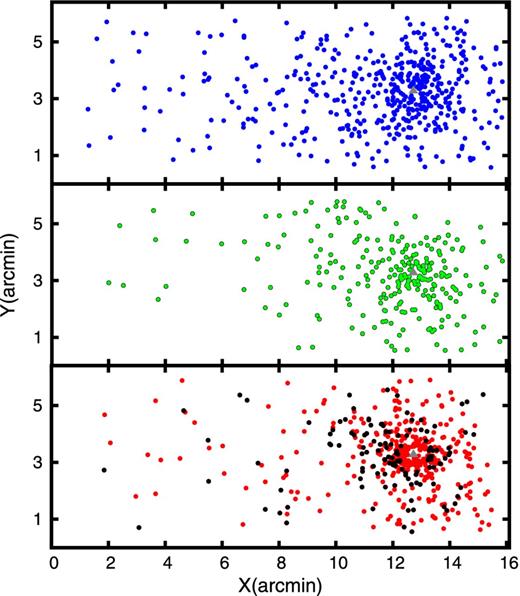
Projected spatial distribution of GC candidates. From top to bottom, the blue, intermediate and red subpopulations, according to the GMM separation. Black filled circles are the GC candidates with (g′ − i′) > 1.16 which show an asymmetric distribution around the centre of NGC 6861. The orientation is the same as Fig. 1.
For the entire sample of candidates, we used concentric circular annuli with Δ log r = 0.1, corrected by background contamination, reaching ∼10 arcmin (∼100 kpc) from the galactic centre. Subsequently, we have obtained separated profiles for the three subpopulations: red, green and blue (Fig. 17). Due to the elongation showed by the red and green subpopulations, the profiles associated with them were obtained using concentric elliptical annuli, according to the PA and ellipticity values obtained in Section 3.6. In the case of blue GC candidates, we did not detect any significant elongation; therefore, we decided to obtain their density profile using circular annuli. It can be seen in Fig. 17 that the red subpopulation presents a stronger spatial concentration towards the galaxy than the blue GCs. On the other hand, blue and green subpopulations show very similar radial profiles. Regarding the extension of the GC system of NGC 6861, Fig. 16 shows candidates at galactocentric distances even larger than 10 arcmin (∼100 kpc). Although at such a distance our areal completeness is small, we cannot rule out that some of them are bona fide GCs.
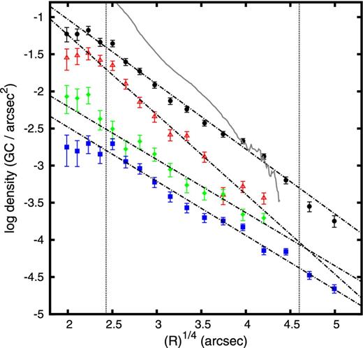
Projected density profile for red (triangles), green (diamond) and blue (squares) subpopulations, and all GC candidates (circles). Solid grey line shows the galaxy starlight profile, which has a similar slope to red clusters. All profiles were fitted with a power law and a de Vaucouleurs law. The vertical dotted lines indicate the range used to make the fits (2.4 < r1/4 < 4.6 arcsec). The profiles were shifted to avoid overlapping.
In order to assess the slope of the profile, we fit a power law and a de Vaucouleurs law (r1/4) to the whole sample, and to the red, green and blue candidates, respectively. We present the obtained values in Table 6. These values are similar to those found in Faifer et al. (2011) for NGC 524 and NGC 3115, and other S0 galaxies (see their table 5). It is interesting to note that the green candidates show identical slopes to the blue ones. However, Fig. 17 shows that green candidates display a possible excess of objects at the inner region of the system, not present in the blue or in the red profiles.
Slope values for power law and de Vaucouleurs law, in the density profiles for the whole sample and for the blue, green and red subpopulations.
| Population | Power law | de Vaucouleurs |
|---|---|---|
| All | −1.60 ± 0.04 | −0.87 ± 0.03 |
| Blue | −1.47 ± 0.07 | −0.73 ± 0.04 |
| Green | −1.35 ± 0.08 | −0.71 ± 0.05 |
| Red | −2.04 ± 0.11 | −1.07 ± 0.08 |
| Population | Power law | de Vaucouleurs |
|---|---|---|
| All | −1.60 ± 0.04 | −0.87 ± 0.03 |
| Blue | −1.47 ± 0.07 | −0.73 ± 0.04 |
| Green | −1.35 ± 0.08 | −0.71 ± 0.05 |
| Red | −2.04 ± 0.11 | −1.07 ± 0.08 |
In summary, from Figs 16 and 17 we can see that the spatial distribution for the blue clusters is radially shallow and circularly symmetric, for the green candidates it is shallow and elliptical, and that for the red GCs is stepper and elliptical.
In order to see if there is any indication of substructure in the spatial distribution of our GC candidates, we analysed the appearance of the xy plots by taking the candidates in different (g′ − i′) colour windows. That exercise has shown that GC candidates with (g′ − i′) > 1.16 present an asymmetric distribution around the centre of NGC 6861. In the lower panel of Fig. 16, we plotted those candidates as black points. In order to quantify this asymmetry, we have done an easy test: we have taken objects with 30 < Rgal < 160 arcsec (complete areal coverage), and then counted them splitting the sample between the left (SE) and the right-hand side of the galaxy (NW). We have got 69 and 35 candidates, respectively. Those numbers show that there are two times more such candidates to the SE of the galaxy centre than to the NW. This could be not a contamination effect because, according to the analysis of our comparison field, we can expect few contaminant objects in that area (<10). Inhomogeneities in GC spatial distributions were reported in other early-type galaxies like NGC 4261, NGC 4649 and NGC 4278 (D'Abrusco et al. 2013a,b; D'Abrusco, Fabbiano & Brassington 2014). These features, like fossil remnants, are strongly suggestive of the accretion and/or merger of some lower mass neighbours.
3.6 Azimuthal properties
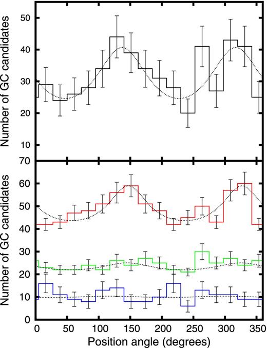
Azimuthal distribution for the entire sample of GC candidates (upper panel), and red, green and blue subpopulations (bottom panel), within a ring around the galaxy as described in the text. In order to avoid overlapping, the curves corresponding to green and red candidates were vertically shifted adding 18 and 35 to the counts.
Values of position angle and ellipticity for the three subpopulations and for the whole sample of GC candidates. In addition, we include the results for X-ray measurements from Machacek et al. (2010).
| Parameter | Blue | Green | Red | All | X | |
|---|---|---|---|---|---|---|
| r ≤ 7.3 kpc | r ≤ 42 kpc | |||||
| PA | – | 145° ± 13° | 146| $_{.}^{\circ}$|8 ± 5° | 137° ± 6° | 128° ± 7° | – |
| e | – | 0.54 ± 0.1 | 0.64 ± 0.04 | 0.52 ± 0.05 | 0.40 ± 0.04 | 0.19 ± 0.05 |
| Parameter | Blue | Green | Red | All | X | |
|---|---|---|---|---|---|---|
| r ≤ 7.3 kpc | r ≤ 42 kpc | |||||
| PA | – | 145° ± 13° | 146| $_{.}^{\circ}$|8 ± 5° | 137° ± 6° | 128° ± 7° | – |
| e | – | 0.54 ± 0.1 | 0.64 ± 0.04 | 0.52 ± 0.05 | 0.40 ± 0.04 | 0.19 ± 0.05 |
Fig. 18 shows that the spatial distribution of the whole sample of GC candidates exhibits strong signs of elongation. The PA is identical within the error to that of the galaxy inside a semi-major axis of 120 arcsec (see Section 3.1). As far as ellipticity is concerned, the values obtained for green, red and all GC candidates are slightly bigger than that of the galaxy. In particular, red candidates show a significantly higher ellipticity than that of the starlight. It is interesting to notice that, according to Fig. 18, the behaviour of the GC candidates is led by the red and green ones. For blue candidates, we did not find any significant elongation and, then, the PA is unconstrained.
3.7 Comparison with the hot gas emission
In their study of the GC systems of the giant elliptical galaxy NGC 1399, Forte, Faifer & Geisler (2005) have shown that there is a similarity between the projected density profile of the blue GC subpopulation and that of the X-ray surface brightness profile of that galaxy. More recently, Forbes, Ponman & O'Sullivan (2012) have extended the study to other eight giant elliptical galaxies and they have found that the same behaviour is present in their sample. Therefore, as far as we are aware, these nine galaxies are the only cases where a direct comparison between the spatial distribution of the blue GCs and the X-ray emission has been made and published. Excluding NGC 720, all of them are massive and giant ellipticals in groups and clusters.
Forte et al. (2007, 2009, 2014) suggested that the red GCs are associated with the bulge stellar component in early-type galaxies, while the blue GCs would be linked to the halo component. In this context, it is natural to think that blue GCs and hot gas can share the same gravitational potential in equilibrium (Forbes et al. 2012). However, it is important to notice that similar projected 2-d distributions do not necessarily imply similar 3-d spatial distribution.
In order to quantitatively compare the slopes of blue GC and X-ray profiles, we have counted blue cluster candidates in concentric circular annuli. Fig. 19 shows counts as small filled circles and the corresponding Poissonian error bars. As a red solid line we plotted the double β-model from Jones et al. (in preparation), shifted vertically to have a good match. As can be seen, the X-ray profile shows an excellent agreement with the blue globular density for r > 50 arcsec (>10 kpc). Subsequently, we have fitted the density profile considering points in the range 10.6 < r < 67.1 kpc by employing a single β-model. The obtained value of the slope is β ∼ 0.38–0.44, which is very similar to that of Machacek et al. However, due to the restricted radial range included in the fit, the rc parameter is not well constrained. In order to obtain a more reliable β-value, we have fitted again the data, but keeping fixed the rc parameter at the value given by Machacek et al. We have obtained β = 0.42 ± 0.01. We plotted this fit as a dashed blue line in Fig. 19. Again, the agreement is excellent showing that outer blue GCs present a similar projected distribution to that of the subgroup X-ray component.
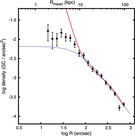
GC density profile for the blue subpopulation (filled black circles) and surface brightness profile in X-ray (red line) of NGC 6861 (Jones et al., in preparation). The profiles were shifted on the vertical axis for a better comparison. Blue dashed line shows the single β-model fitted to the GC density. The agreement between the blue GC and X-ray profiles outside 10 kpc is remarkable.
3.8 Luminosity function
The adopted distance of 28.1 Mpc for NGC 6861 in this work translates in a distance modulus of (m − M) = 32.24 mag. Therefore, taking an approximated turnover (TO) of MV = −7.5 mag (e.g. Harris 2001), and equation (2) from Faifer et al. (2011), we estimated a value for the peak of the GC luminosity function (GCLF) in the g′ band at ∼25.1 mag. As we showed in Section 2.4, the completeness of our photometry is greater than 80 per cent for |$g^{\prime }_0<$| 25.5 mag. This indicates that we will be able to obtain a good representation of the integrated GCLF for NGC 6861.
In order to do that, we counted candidates in bins of 0.25 mag. This raw luminosity distribution is shown in Fig. 20 as a dotted line histogram. Subsequently, we have corrected the counts for completeness effects and background contamination and plotted it as solid histograms in Fig. 20. This figure shows that a peak around |$g^{\prime }_0\sim 25$| mag is clearly detected.
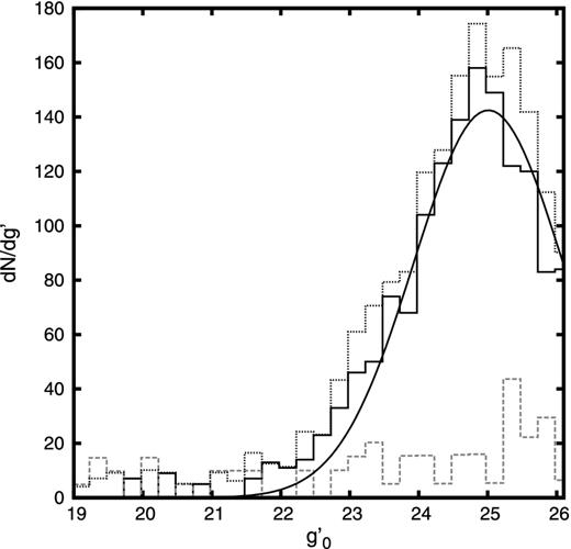
The dotted histogram shows counts of GC candidates considering bins of 0.25 mag. After applying completeness and background corrections, we obtain the solid line histogram. The adopted normalized background is shown as a dashed histogram. The solid line represents the Gaussian fit to the corrected GCLF.
Although different options exist in the literature to model the GCLF (see Jordán et al. 2007), we have adopted here a Gaussian form. The main reason behind this election is that there is a historic use of Gaussian representation as distance indicator (Jacoby et al. 1992; Villegas et al. 2010). Therefore, we fitted a Gaussian function to our histogram, and determined the position of the TO magnitude and the dispersion of the GCLF. In the fit, we included all the bins with magnitude g′ < 26.2 mag. The values obtained for both parameters are listed in Table 8, and Fig. 20 shows the obtained fit. The value of |$\sigma _g^{\prime }$| is in very good agreement with the relation between the intrinsic Gaussian dispersion of the g-band GCLF, and the absolute blue magnitude of the parent galaxy, σg − MB, presented in fig. 9 of Jordán et al. (2007).
Parameters obtained by fitting Gaussian functions to the g′-band GCLF. Turnover magnitude (TO) and dispersion (σ) for the whole sample, and blue and red subpopulations are shown.
| Population | TO | σ |
|---|---|---|
| All | 25.00 ± 0.05 | 1.08 ± 0.06 |
| Blue | 24.70 ± 0.06 | 1.00 ± 0.06 |
| Red | 25.18 ± 0.08 | 1.07 ± 0.08 |
| Population | TO | σ |
|---|---|---|
| All | 25.00 ± 0.05 | 1.08 ± 0.06 |
| Blue | 24.70 ± 0.06 | 1.00 ± 0.06 |
| Red | 25.18 ± 0.08 | 1.07 ± 0.08 |
Our next step was to obtain the GCLF for the different subpopulations detected in NGC 6861. Fig. 21 shows the blue and red corrected histograms and the fitted Gaussian models. As we did not detect any difference between the fit for the green and red candidates, we considered both subsamples together in the fit. The values of the obtained parameters are listed in Table 8.
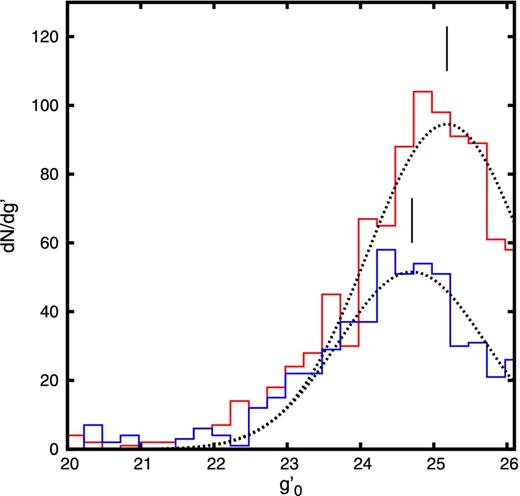
Corrected LF for blue and red subpopulations. Dotted lines and vertical short lines represent the Gaussian fit and TO magnitude, respectively.
It is interesting to notice that we have obtained a significant difference between the TO magnitudes of blue and red clusters. We can see from Table 8 that TOred − TOblue ∼ 0.48 mag. It is immediate to think in the existence of metallicity effects behind this result. Ashman, Conti & Zepf (1995) have investigated the shift in the peak of the GCLF as a function of metallicity for the B, V, R, I and J filters. They based their results on simulations that included the cluster masses drawn from a parent population similar to that of the MW, and a mean metallicity ranging from −0.2 to −1.6 dex. According to their table 3, and assuming mean [Fe/H] of −1.6 and −0.6 dex for the blue metal-poor and red metal-rich GCs, respectively, we can expect a TO shift of around 0.3 mag in the V band. Red GCs in NGC 6861 are probably more metal rich than those of the MW. Therefore, the TO shift in this S0 galaxy could be larger than that in our galaxy. Unfortunately, Ashman et al. (1995) did not include the Sloan filters in their calculations. For that reason, we transformed the TO magnitudes for blue and red GCs using equation (2) from Faifer et al. (2011), and adopting as mean colours 0.78 and 1.13 mag for blue and red candidates, respectively. This translates in a 0.43 mag shift for the TO magnitude in the V band. If we assume that blue GCs in NGC 6861 are similar to those of the MW, according to fig. 7 of Rejkuba (2012), the mean metallicity of red GC in this galaxy should be ∼−0.25 dex.
This result shows that it may not be a good idea to measure distances using the GCLF obtained in blue bands for the whole sample. It is possible to minimize the metallicity effect by observing in the near-IR regime (like z; Villegas et al. 2010). However, another option is to use the TO magnitude of the blue GCs as a distance indicator. Di Criscienzo et al. (2006) have shown that adopting a common Large Magellanic Cloud fiducial distance scale of (m − M) = 18.50 mag, the TO magnitudes of metal-poor GCLF in the MW, M31 and the more distant galaxy sample of Larsen et al. (2001) are in perfect mutual agreement with MV = −7.66 mag.
Taking Di Criscienzo et al. (2006) TO magnitude for the blue GCs, the corresponding mean (g′ − i′) colours from Table 5 and using equation (2) from Faifer et al. (2011), we got |$M_{g^{\prime }}$| = −7.39 mag. With this value and the apparent magnitude for the TO of the blue GCLF from Table 8, we got a distance modulus of (m − M) = 32.1 mag. This value is in very good agreement with that of Tonry et al. (2001), (m − M) = 32.24 ± 0.36 mag.
3.9 Total number of GCs and specific frequency
In Section 3.5, we determined the density profiles for the different subpopulations and for the whole system. By extrapolating the density profile from ∼30 to 600 arcsec, we got 1834 GCs. The last value is equivalent to ∼100 kpc at the adopted distance of NGC 6861. We have taken this external cut because the analysis presented in that subsection showed that there are GCs even at such a large galactocentric distance. Besides, that value is in agreement with several wide-field studies of different GC systems of massive galaxies (Bassino et al. 2006; Harris 2009b). In the inner region (≲30 arcsec), we assume that the density of GCs is constant. This gives us 160 more GCs.
These 1994 GCs, according to the TO value obtained for the whole sample of candidates, correspond to 67 per cent of GCs brighter than |$g^{\prime }_0$| = 25.5 mag, leaving 33 per cent fainter. Considering a ±20 per cent variation in the extension of the surface density profile due to the uncertainties in their parameters, by integrating the LF profile over all magnitudes, we estimate a total number of 3000 ± 300 GCs.
Therefore, for NGC 6861 we obtain a surprisingly high value of SN = 9.2 ± 2.2. On the other hand, if we adopt the distance modulus obtained from the TO magnitude for blue GCs in the previous section, we get MV = −21.12 mag and SN = 10.6 ± 2.1. These are extremely high values of SN, similar to that of giant cluster dominant early-type galaxies like M87. Harris, Harris & Alessi (2013) presented a compilation of global properties of GC systems. We can see that there are only two S0 galaxies with D < 100 Mpc and MV < −20 mag which present SN > 7 in that sample. They are NGC 1400 and IC 3651. However, checking the source with those values, we can see that in the case of NGC 1400, Perrett et al. (1997) found Nt = 922 ± 280 GCs and SN = 5.2 ± 2. On the other hand, Marín-Franch & Aparicio (2002) list a value of SN = 5.7 ± 1.8 for IC 3651. However, this relies on an indirect estimation of MV for that galaxy as it does not appear in the RC3 catalogue, and on an indirect estimation of Nt using the surface brightness fluctuation method. In this context, NGC 6861 seems to be a more definite case of a high-SN lenticular galaxy.
High SN values are usually found in low- and high-mass early-type galaxies. This is evident in the ‘U’ shape plot of SN versus MV like that presented in fig. 10 in Harris et al. (2013). As SN measures the formation efficiency of GCs relative to field stars, high-SN galaxies can be understood as ‘field-stars-deficient’ or ‘cluster-rich’ systems. However, several studies provided growing evidence in favour of the first situation. Specifically, McLaughlin (1999) has shown that the enhanced SN value for the most massive galaxies in his sample can be accounted for if the mass in GCs is normalized to the total baryonic mass of the host (i.e. X-ray emitting gas and the stellar component), ϵ = MGCs/Mb ∼ 0.0026. In this context, according its SN value, NGC 6861 could have a massive baryonic halo associated with the hot gas emitting in X-ray.
Recently, a more fundamental ratio was defined: the ratio of the mass in GCs to the total galaxy halo mass, η = MGCs/Mh. This ratio seems to be essentially constant over the whole mass range of galaxies (Georgiev et al. 2010; Harris et al. 2013). Using a comprehensive data base of 307 galaxies, Hudson, Harris & Harris (2014) confirmed this suggestion through a new calibration of galaxy halo masses entirely based on weak lensing. They obtained a value of 〈η〉 = 3.9 ± 0.9 × 10⁻⁵. Following Harris et al. (2013) we estimated the total mass enclosed in the GCS of NGC 6861 (adopting (M/L)V = 2), MGCs = 9 ± 1 × 10⁸ M⊙, and therefore we used the 〈η〉 value to estimate the total mass of the halo of NGC 6861. We found Mh = 2.3 ± 0.5 × 10¹³ M⊙. This value indicates again that according to its GC system, we can expect a massive halo in NGC 6861.
4 CONCLUSIONS
Using deep images taken with Gemini/GMOS, we obtained multicolour photometry of three fields around NGC 6861. This galaxy presents unique features for an S0 type, summarized as follows.
NGC 6861 presents signs of past interaction or merger, like the non-concentric isophotes shown by the galaxy. In addition, we have found several different structures that become visible when the ratio between the original image and the smooth ellipse model is analysed.
The galaxy has a large GC system which extends up to 100 kpc. By analysing the colour–colour and colour–magnitude diagrams, we detected at least two subpopulations of GC, blue and red, with colour peaks at (g′ − i′)0 ∼ 0.79 and (g′ − i′)0 ∼ 1.07 mag, respectively. By examining the colour histograms and the CMD, we inferred the possible existence of a third subpopulation with intermediate colours ((g′ − i′)0 ∼ 0.95). We have tentatively separated the cluster candidates in blue, green and red subpopulations. However, spectroscopic and/or IR data are needed to perform an age–metallicity study, and confirm or rule out the existence of this third subpopulation.
The presence of a blue tilt is detected in the blue subpopulation, probably being the first case in this galaxy type.
Regarding the spatial distribution of the blue and green subpopulations, their density profiles show similar slopes.
Outside 10 kpc, the blue subpopulation shows a remarkable similarity between the projected density profile and the X-ray surface brightness profile of the galaxy. This result would indicate that NGC 6861 could be the dominant galaxy in a galaxy subgroup, as mentioned by Machacek et al. (2010).
The azimuthal distribution of the red and green GC candidates exhibits strong signs of elongation, with an ellipticity slightly larger than that of the galaxy.
By comparing the galaxy light with the red subpopulation, we can see that in the inner region they both share similar features such as PA, colour and slope of the density profile.
Red GC candidates with colours (g′ − i′)0 > 1.16 show an asymmetric spatial distribution around the galaxy. Similar features were reported in other galaxies, suggesting accretion and/or merger of a lower mass neighbour.
We obtained the global GCLF of NGC 6861, as well as for the blue and red subpopulations separately. A significant difference between the TO values of both subpopulations in the g′ band was obtained (TOred − TOblue ∼ 0.48 mag). The existence of metallicity effects might be behind this result.
Using the blue GC candidates, we estimated a new distance modulus (m − M = 32.1 mag), which shows a good agreement with that of Tonry et al. (2001).
We have estimated a total population of 3000 ± 300 GCs for NGC 6861.
From the distance given by Tonry et al. (2001), we obtained a high specific frequency of SN = 9.2 ± 2.2, and from our own distance estimation, a higher value of SN = 10.6 ± 2.1. As far as we know, this is the highest SN measured for a lenticular galaxy up to date. This high SN value could be interpreted as a sign of the presence of a massive halo in NGC 6861.
We warmly thank M. Machacek for providing the X-ray surface brightness profile of NGC 6861, and Sergio Cellone and Analia Smith Castelli for reading of the manuscript and several useful comments. This work was funded with grants from Consejo Nacional de Investigaciones Cientificas y Tecnicas de la Republica Argentina and Universidad Nacional de La Plata (Argentina). This work is based on observations obtained at the Gemini Observatory, which is operated by the Association of Universities for Research in Astronomy, Inc., under a cooperative agreement with the NSF on behalf of the Gemini partnership: the National Science Foundation (United States), the National Research Council (Canada), CONICYT (Chile), the Australian Research Council (Australia), Ministério da Ciência, Tecnologia e Inovação (Brazil) and Ministerio de Ciencia, Tecnología e Innovación Productiva (Argentina). The Gemini programme ID are GS-2010B-Q-2 and GS-2011A-Q-81. This research has made use of the NED, which is operated by the Jet Propulsion Laboratory, Caltech, under contract with the National Aeronautics and Space Administration.
iraf is distributed by the National Optical Astronomical Observatories, which are operated by the Association of Universities for Research in Astronomy, Inc., under cooperative agreement with the National Science Foundation.
rmix is publicly available at http://www.math.mcmaster.ca/peter/mix/mix.html
