


Abstract
We obtain predictions for the properties of cold dark matter annihilation radiation using high-resolution hydrodynamic zoom-in cosmological simulations of Milky Way-like galaxies (apostle project) carried out as part of the ‘Evolution and Assembly of GaLaxies and their Environments’ (eagle) programme. Galactic haloes in the simulation have significantly different properties from those assumed in the ‘standard halo model’ often used in dark matter detection studies. The formation of the galaxy causes a contraction of the dark matter halo, whose density profile develops a steeper slope than the Navarro–Frenk–White (NFW) profile between r ≈ 1.5 kpc and r ≈ 10 kpc. At smaller radii, r ≲ 1.5 kpc, the haloes develop a flatter than NFW slope. This unexpected feature may be specific to our particular choice of subgrid physics model but nevertheless the dark matter density profiles agree within 30 per cent as the mass resolution is increased by a factor 150. The inner regions of the haloes are almost perfectly spherical (axis ratios b/a > 0.97 within r = 1 kpc) and there is no offset larger than 45 pc between the centre of the stellar distribution and the centre of the dark halo. The morphology of the predicted dark matter annihilation radiation signal is in broad agreement with γ-ray observations at large Galactic latitudes (b ≳ 3°). At smaller angles, the inferred signal in one of our four galaxies is similar to that which is observed but it is significantly weaker in the other three.
1 INTRODUCTION
Uncovering the unknown nature of the dark matter is one of the greatest challenges of modern cosmology and particle physics. Since the original suggestion that the dark matter might consist of massive, cold, weakly interactive, neutral particles, a large body of empirical evidence has consolidated this hypothesis which, however, can only be confirmed by the detection of the particles themselves. Among the possible candidates, supersymmetric particles (see Jungman, Kamionkowski & Griest 1996, for a review) such as neutralinos are attractive options that current particle accelerator experiments might detect.
An interesting property of many particle candidates for cold dark matter (CDM) is that they annihilate into standard model particles, including photons. This opens up the exciting possibility of attempting to detect such photons from space. The requirement that weakly interacting particles provide the measured dark matter density in the Universe today suggests a plausible particle mass range of order mχ = 10–1000 GeV, leading to the emission of γ-ray photons in or below that energy range when two dark matter particles annihilate (see review by Bertone, Hooper & Silk 2005).
The Large Area Telescope aboard the Gamma-Ray Space Telescope (Fermi; Gehrels & Michelson 1999) has, over the last few years, produced the most detailed maps of the γ-ray sky, covering a large energy range (|$20\ \rm {MeV}{\rm -}500\ \rm {GeV}$|) with a resolution of a few arcmin at the highest energy end of the spectrum. Analysing the Fermi data around the Galactic Centre (GC), a number of authors (Goodenough & Hooper 2009; Hooper & Goodenough 2011; Hooper & Linden 2011; Abazajian & Kaplinghat 2012; Gordon & Macías 2013; Hooper & Slatyer 2013; Abazajian et al. 2014; Daylan et al. 2014; Macias & Gordon 2014; Calore, Cholis & Weniger 2015) have claimed the detection of extended diffuse excess emission above the other known astrophysical sources. This excess emission, peaking at E ≈ 2 GeV, was found to be broadly consistent with the expected signal from dark matter annihilation. In particular, the flux decreases with distance from the GC as r−Γ with slope, Γ = 2.2–2.4, only slightly steeper than the asymptotic inner slope, Γ = 2, of flux originating from the NFW (Navarro, Frenk & White 1996b, 1997) density profiles found in dark matter only simulations of haloes.
However, potential systematic effects in the analysis of the γ-ray data could be introduced by incorrect point source subtraction or the modelling of the diffuse backgrounds (Ackermann et al. 2012). Alongside the dark matter interpretation of the GC excess, astrophysical explanations have been proposed. For example, a population of as yet unresolved millisecond pulsars (MSP; Abazajian 2011; Gordon & Macías 2013; Yuan & Zhang 2014; Cholis, Hooper & Linden 2015a) or young pulsars (O'Leary et al. 2015) associated with the bulge1 of the Milky Way (MW). In contrast to the conclusions of Hooper et al. (2013) and Cholis et al. (2015a), Bartels, Krishnamurthy & Weniger (2015) and Lee et al. (2015) have argued that the excess could be due to such a pulsar population. Alternatively, Linden, Lovegrove & Profumo (2012), Carlson & Profumo (2014), Petrović, Dario Serpico & Zaharijaš (2014) and Cholis et al. (2015b) have suggested that the excess could originate from the injection of very high energy cosmic rays during past activity in the GC.
Besides the spectral shape, another property that can help distinguish the potential sources of γ-rays contributing to the excess is the morphology of the signal. A dark matter origin would require the excess to extend over tens of degrees on the sky (Serpico & Zaharijas 2008; Springel et al. 2008b; Nezri, Lavalle & Teyssier 2012). An excess with the same spectral shape extending over a large angular range, with emissivity decreasing with distance from the GC, would strengthen the interpretation of the excess as originating from dark matter annihilation. Using multiple regions between 2° and 20° from the GC and a large range of Galactic diffuse emission (GDE) models, Calore et al. (2015) found that the excess emission is consistent with a dark matter particle of mass |$m_\chi =49^{+6.4}_{-5.4}\ \rm {GeV}$| annihilating into a |$b\bar{b}$| quark pair then producing photons and is distributed following a generalized NFW profile (gNFW, see equation 1 below) with a slope γ = 1.26 ± 0.15. A similar spatial distribution was found by Daylan et al. (2014) who suggested a slope for the inner profile in the range γ = 1.1–1.3. With the increasing precision of these measurements and of the foreground modelling, it has become crucial to refine the theoretical models for the distribution of dark matter at the centre of galaxies in a ΛCDM context. Characterizing the dark matter profile slope and sphericity as well as investigating the potential offset between the dark matter and the GC are all important tasks for theorists.
Work based on dark matter only simulations has shown that the dark matter is distributed following an NFW density profile with a scalelength, rs, which varies with halo mass (e.g. Navarro et al. 1997; Neto et al. 2007; Duffy et al. 2008; Dutton & Macciò 2014). Higher resolution simulations (Springel et al. 2008a) have shown that the very inner parts of dark matter profiles might be slightly shallower than the asymptotic NFW slope of γ = 1 (Navarro et al. 2010). Similarly, predictions for the signal coming from subhaloes have also been made using these simulations (Kuhlen, Diemand & Madau 2008; Springel et al. 2008b), effectively proposing a test of the CDM paradigm. At the other end of the halo mass range, Gao et al. (2012) argued that nearby rich clusters provide a signal with a higher signal-to-background ratio than the MW's satellites. Thus, far observational measurements have proved inconclusive and the only claimed detection comes from the centre of our own MW, where precise predictions from dark matter simulations have been made (Springel et al. 2008b).
However, these studies all ignored the effects of the forming galaxy on the structure of the dark matter halo. Mechanisms such as dark matter contraction (e.g. Barnes & White 1984; Blumenthal et al. 1986; Gnedin et al. 2004) can drag dark matter towards the centre, steepening the profile. Conversely, perturbations to the potential, due for instance to feedback from stars or supermassive black holes or the formation of a bar, can lead to a flattening of the very central regions (e.g. Navarro, Eke & Frenk 1996a; Weinberg & Katz 2002; Mashchenko, Couchman & Wadsley 2006; Pontzen & Governato 2012). The correct balance between these mechanisms can only be understood by performing high-resolution hydrodynamic simulations of MW-like galaxies using a physical model validated by comparison with a wide range of other observables.
In this study, we use two ‘zoom’ simulations of Local Group environments (the apostle project; Fattahi et al. 2015; Sawala et al. 2015) performed within the framework of the ‘Evolution and Assembly of GaLaxies and their Environments’ (eagle) suite (Crain et al. 2015; Schaye et al. 2015). These simulations have been shown to reproduce a large number of observables of the galaxy population at low and high redshifts, as well as the satellite galaxy luminosity functions of the MW and Andromeda galaxies with unprecedented accuracy. Schaller et al. (2015a) showed that the eagle simulations produce galaxies with rotation curves that are in unprecedented agreement with observations of field galaxies, suggesting that the matter distribution in the simulated galaxies is realistic and that the main effects of baryons on haloes are accurately captured by the simulations. Note, however, that Calore et al. (2015a) showed that the goodness of fit of the simulated data to the observed MW rotation curve is lower in the highest resolution zoomed-in simulations. The eagle simulations therefore provide an excellent test-bed for the interpretation and analysis of the Fermi excess.
This paper is structured as follows. In Section 2, we introduce the simulation setup used. We investigate the dark matter density profiles of our haloes in Section 3 and analyse the dependence of the annihilation signal on the angle with respect to the GC in Section 4. We summarize our findings and conclude in Section 5.
Throughout this paper, we assume a Wilkinson Microwave Anisotropy Probe7 flat ΛCDM cosmology (Komatsu et al. 2011, h = 0.704, Ωb = 0.0455, Ωm = 0.272 and σ8 = 0.81), express all quantities without h factors and assume a distance from the GC to the Sun of r⊙ = 8.5 kpc.
2 THE SIMULATIONS
The simulations used in this study are based on the eagle simulation code (Crain et al. 2015; Schaye et al. 2015). We summarize here the parts of model relevant to our discussion.
2.1 Simulation code and subgrid models
The eagle code is based on a substantially modified version of the gadget code, last described by Springel (2005). The modifications include the use of a state-of-the-art implementation of smoothed particle hydrodynamics (SPH), called anarchy (Dalla Vecchia, in preparation; see also Schaller et al. 2015c), based on the pressure–entropy formulation of SPH (Hopkins 2013). Gravitational interactions are computed using a Tree-PM scheme.
The cooling of gas and its interaction with the background radiation is implemented following the recipe of Wiersma, Schaye & Smith (2009a) who tabulated photoheating and cooling rates element-by-element (for the 11 most important elements) in the presence of the ultraviolet and X-ray backgrounds inferred by Haardt & Madau (2001). To prevent artificial fragmentation, a pressure floor in the form of an effective equation of state, Peos ∝ ρ4/3, designed to mimic the mixture of phases in the interstellar medium (ISM; Schaye & Dalla Vecchia 2008), is applied to the cold and dense gas. Star formation is implemented using a pressure-dependent prescription that by construction reproduces the observed Kennicutt–Schmidt star formation law (Schaye & Dalla Vecchia 2008) and uses a density threshold that captures the metallicity dependence of the transition from the warm, atomic to the cold, molecular gas phase (Schaye 2004). Star particles are treated as single stellar populations with a Chabrier (2003) initial mass function evolving along the tracks advocated by Portinari, Chiosi & Bressan (1998). Metals from supernovae (SNe) and AGB stars are injected into the ISM following the model of Wiersma et al. (2009b) and stellar feedback is implemented via the stochastic injection of thermal energy into the gas neighbouring newly formed star particles as described by Dalla Vecchia & Schaye (2012). Galactic winds hence form naturally without having to impose a direction, velocity or mass loading factor. The amount of energy injected into the ISM per feedback event is dependent on the local gas metallicity and density in an attempt to take into account the unresolved structure of the ISM (Crain et al. 2015; Schaye et al. 2015). Supermassive black hole seeds are injected in haloes above 1010h−1 M⊙ and grow through mergers and the accretion of low angular momentum gas (Rosas-Guevara et al. 2015; Schaye et al. 2015). Active galactic nucleus (AGN) feedback is modelled by stochastically injecting thermal energy into the gas directly surrounding the black hole (Booth & Schaye 2009; Dalla Vecchia & Schaye 2012). Haloes are identified using the Friends-of-Friends algorithm (Davis et al. 1985) and substructures within them are identified in post-processing using the subfind code (Dolag et al. 2009).
The subgrid model was calibrated (by adjusting the efficiency of stellar feedback and the accretion rate on to black holes) so as to reproduce the present day stellar mass function and galaxy sizes, as well as the relation between galaxy stellar masses and supermassive black hole masses (Crain et al. 2015; Schaye et al. 2015). As argued by (Schaye et al. 2015, section 2), numerical convergence in the traditional sense (strong convergence) cannot be achieved when new physical processes are resolved at each resolution. In this case, the free parameters of the model should be recalibrated to match the same pre-defined set of observables (weak convergence). This can be done in cosmological simulations of representative periodic volumes (Crain et al. 2015), but it is much more difficult to achieve for ‘zoom-in’ simulations of a few objects. In this case, even weak convergence is difficult to establish (see Section 3.3).
2.2 Selection of MW haloes
The two volumes used in this work are zoom resimulations of regions extracted from a dark matter only simulation of 1003 Mpc3 with 16203 particles. The haloes were selected to match the observed dynamical constraints of the Local Group (apostle project; Fattahi et al. 2015; Sawala et al. 2015). Each volume contains a pair of haloes in the mass range M200 = 5 × 10¹¹ M⊙ to M200 = 2.5 × 10¹² M⊙ that will host analogues of the MW and M31. We use the two haloes in volumes AP-1 and AP-4 of the apostle suite (see table 2 of Fattahi et al. 2015, where other relevant data are listed). The high-resolution region encloses a sphere larger than 2.5 Mpc around the centre of mass of the two haloes at z = 0. The dark matter particle mass in the zoom regions was set to 5 × 10⁴ M⊙, whilst the primordial gas particle mass was set to 1 × 10⁴ M⊙. The initial conditions were generated from ΛCDM power spectra using second-order Lagrangian perturbation theory (Jenkins 2010) and linear phases were taken from the Gaussian white noise field panphasia (Jenkins 2013). The gravitational softening length was set to ϵ = 134 pc (Plummer equivalent) at z < 2.8 and was kept fixed in comoving units at higher redshifts. Simulations without baryonic components were run with the exact same setup and are labelled as dmo in what follows.
3 DARK MATTER DISTRIBUTION IN THE CENTRE OF THE HALOES
In this section, we analyse the dark matter distribution of the haloes of simulated MW galaxies. We consider both central galaxies in each of the two simulation volumes as MW-like galaxies.
3.1 Profiles without baryon effects
In order to quantify the effects of baryons on the dark matter distribution, it is worth first considering the profiles extracted from the simulations without baryonic physics. In Fig. 1, we show the dark matter density profiles of our four haloes. Thick lines are used at radii greater than the resolution limit (RP03 ≈ 350-450 pc depending on the halo) set by the criterion of Power et al. (2003) and thin lines are used at smaller radii. The softening length is indicated by the vertical dotted line. The green dot–dashed and blue dashed lines correspond to NFW and gNFW with γ = 1.26 (the best-fitting value of Calore et al. (2015) to the excess) profiles, respectively, both normalized, as discussed above, to ρDM(r⊙) = 0.4 GeV cm−3 and with a scalelength rs = 20 kpc. As expected, the profiles are in good agreement with the NFW model albeit with a lower normalization. The best-fitting NFW profile parameters to our haloes are given in Table 1. The usual choice of rs = 20 kpc is in good agreement with our simulated haloes but the normalization of our haloes is lower than what is often assumed in the literature. When baryon effects are neglected, an inner slope close to γ = 1.26 is clearly incompatible with the simulations.
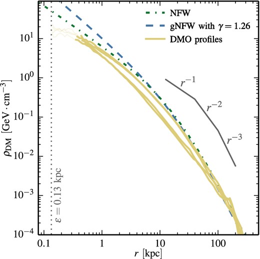
The dark matter density profiles of the four haloes in the simulations without baryons (yellow solid lines). Thinner lines are used at radii smaller than the convergence radius of the simulation. The vertical dotted line indicates the simulation's gravitational softening length. The green dot–dashed and blue dashed lines correspond to an NFW and gNFW with γ = 1.26 profiles, respectively, both normalized to ρ(r⊙) = 0.4 GeV cm−3 and with a scalelength rs = 20 kpc. As expected, the simulated profiles display a shape similar to the plotted NFW model, but with a lower normalization than the standard haloes.
Properties of the four simulated dmo haloes (Fig. 1) and the best-fitting NFW parameters to their dark matter density profiles. The spherical overdensity masses and radii are given with respect to the critical density of the universe.
| Halo | M200 | R200 | RP03 | rs | ρDM(r⊙) |
|---|---|---|---|---|---|
| ( M⊙) | (kpc) | (pc) | (kpc) | |$(\rm {GeV}\,\rm {cm}^{-3})$| | |
| 1 | 1.65 × 10¹² | 243.2 | 435 | 22.4 | 0.290 |
| 2 | 1.09 × 10¹² | 212.0 | 445 | 20.1 | 0.132 |
| 3 | 1.35 × 10¹² | 226.9 | 344 | 23.2 | 0.162 |
| 4 | 1.39 × 10¹² | 229.4 | 358 | 19.8 | 0.281 |
3.2 Profiles in the simulations with baryons
We now turn towards the dark matter profiles in the simulations including baryons. In Fig. 2, we show the dark matter density profiles of the four haloes simulated with the full baryonic model. As for the previous figure, the lines are thin at radii less than the convergence radius of the simulation RP03 and the dashed lines correspond to the NFW and gNFW profiles normalized to ρ(r⊙) = 0.4 GeV cm−3. The simulated profiles present two interesting features when compared to the dmo results. In the range 1.5-10 kpc, the profile is significantly steeper than an NFW profile and at radii r ≲ 1 kpc, the profiles display a significant flattening. Our profiles thus display a combination of dark matter contraction and a flattening further in. The properties of the dark matter distribution in the central regions are, however, particularly sensitive to the choice of subgrid model so these results, particularly the flattening of the profile, should be regarded as tentative and, by no means, as a generic prediction of ΛCDM.
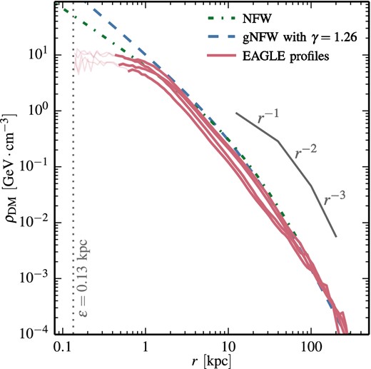
The dark matter density profiles of the four haloes in the simulations with baryons physics (red solid lines). Thinner lines are used at radii smaller than the convergence radius of the simulation. The vertical dotted line indicates the simulation's gravitational softening length. The green dot–dashed and blue dashed lines correspond to an NFW and gNFW with γ = 1.26 profiles, respectively, both normalized to ρ(r⊙) = 0.4 GeV cm−3 and with a scalelength rs = 20 kpc. The profiles display a logarithmic slope steeper than −1 between r ≈ 1.5 kpc and r ≈ 10 kpc, in broad agreement with the profiles inferred from observations by Calore et al. (2015). At radii r ≤ 1 kpc the profile is significantly shallower than NFW profiles are.
These haloes are clearly not well described over their entire radial range by any of the profiles commonly found in the literature. The main properties of the haloes are given in Table 2. Note that in agreement with the findings of Schaller et al. (2015a) for the lower resolution periodic eagle volume, the halo masses M200 (and hence radii R200) are lower than in the simulation that did not include baryon physics. A consequence of the steepening of the profile due to contraction is the slight increase in the local dark matter density ρDM(r⊙) (column 6 of the tables), which, however, remains lower than the commonly adopted value of |$0.4\ \rm {GeV}\,\rm {cm}^{-3}$| in each case. Clearly, the simulated profiles will not be well described by a gNFW profile at radii r ≲ 1.5 kpc. It is, however, instructive to find the best-fitting profile at larger radii for comparison with the models used to characterize the Fermi excess. The best-fitting asymptotic slopes are given in column 5 of Table 2. For all four haloes, the slopes are steeper than the value (γ = 1.26 ± 0.15) found by Calore et al. (2015) when modelling the GC excess. We note, however, that the simulated profiles are in broad agreement with the gNFW profile of (Calore et al. 2015, blue dashed line), if the overall normalization is, once again, ignored. The baryons significantly steepen the profiles at radii r ≳ 1.5 kpc.
Properties of the four simulated eagle haloes (Fig. 2) and the best-fitting gNFW asymptotic slope γ to their dark matter density profiles in the radial range r > 1.5 kpc.
| Halo | M200 | R200 | RP03 | γ | ρDM(r⊙) |
|---|---|---|---|---|---|
| ( M⊙) | (kpc) | (pc) | ( − ) | |$(\rm {GeV}\,\rm {cm}^{-3})$| | |
| 1 | 1.56 × 10¹² | 238.8 | 559 | 1.38 | 0.310 |
| 2 | 1.01 × 10¹² | 206.8 | 592 | 1.47 | 0.160 |
| 3 | 1.12 × 10¹² | 213.7 | 438 | 1.73 | 0.204 |
| 4 | 1.16 × 10¹² | 216.2 | 462 | 1.49 | 0.280 |
At radii r ≲ 1.5 kpc, the density profiles deviate significantly from the cusp seen in the dmo simulation. At the resolution limit, RP03 = 450–600 pc, the simulated profiles exhibit a density between 2.5 and 4.2 times lower than the best-fitted gNFW profile inferred from observations. This flattening is an important feature since the densest regions of the haloes dominate the γ-ray emission. No such flattening was seen in the reference eagle simulations, which, however, had over 200 times poorer mass resolution than the Local Group apostle simulations used here. Here, the flattening is well resolved since it occurs at radii significantly larger than the Power et al. (2003) convergence radius. This indicates that the flattening is not a result of poor sampling but rather a consequence of our specific choice of subgrid model.
At high redshift, all four examples had developed the cuspy central profile that is characteristic of dark matter haloes. However, the inner profiles flattened during events that are clearly associated with violent star formation in the inner few kiloparsecs. In one example, the cusp regenerated before being flattened again by a new episode of violent star formation activity. This phenomenon is reminiscent of the cusp-destroying mechanism proposed by Navarro et al. (1996a) in which the sudden removal of dense, self-gravitating gas from the centre by a starburst redistributes the binding energy of the central regions. Related processes have been seen in recent simulations, mostly of dwarf galaxies (e.g. Duffy et al. 2010; Governato et al. 2010; Macciò et al. 2012; Pontzen & Governato 2012; Teyssier et al. 2013; Oñorbe et al. 2015). We defer a detailed discussion of the causes of this interesting phenomenon to a separate study.
3.3 Resolution and convergence considerations
In the previous two subsections, we used the criterion of Power et al. (2003) as the resolution limit of our simulations. This criterion, based on the two-body relaxation time-scale, was derived using purely collisionless simulations and was designed to ensure that the enclosed mass at a given radius, RP03, is within 10 per cent of the value obtained using a higher resolution simulation. In the cases, where baryonic effects are simulated, it is unclear whether this criterion still applies and even whether numerical convergence in the usual sense can be achieved (see discussion in Schaye et al. 2015). Schaller et al. (2015a) demonstrated that stacked haloes, extracted from the eagle volumes, are well converged when using this simple criterion but it is unclear whether this remains true when individual haloes are considered. Of particular concern is the use of the pressure floor for the densest gas, which sets an artificial scale below which gas cannot be compressed. For our simulations, at all resolutions, this pressure floor ensures that Jeans lengths above λJ ≈ 750 pc can be resolved and prevents the collapse of gas clouds of smaller sizes. It is therefore possible that the profiles may be modified by this pressure floor at radii r ∼ λJ, which, incidentally, is similar to the value of RP03 in our highest resolution simulation.
In Fig. 3, we show the density profiles (multiplied by r2 to reduce the dynamic range) of the dark matter extracted from one of our simulations run at three different resolutions, separated by factors of 12 in particle mass. The bottom set of curves are extracted from the simulation without baryons (and have been multiplied by a factor 0.2 for clarity), whilst the upper set of lines are taken from the simulations with baryons. Dashed lines are used at radii r < RP03 and the vertical dotted lines indicate the softening lengths in each of the three simulations. As a guide, NFW profiles with rs = 20 kpc and the same value of ρDM(r⊙) as the highest resolution simulation are shown using yellow lines. Similar figures for the three other haloes are shown in Appendix A.
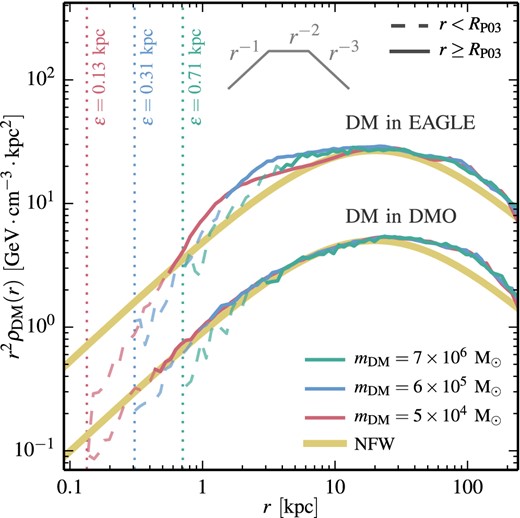
Convergence test for the dark matter profiles of one of the haloes (Halo 1) in both the simulation with baryons (upper set of lines) and without baryons (lower set of lines, rescaled by a factor of 0.2 for clarity). The green, blue and red lines correspond to the simulations with a dark matter particle mass of 7 × 10⁶ M⊙, 6 × 10⁵ M⊙ and 5 × 10⁴ M⊙, respectively. Dashed lines are used at radii smaller than the convergence radius, RP03, of each resolution. The vertical dotted lines indicate the softening length of each simulation. The thick yellow lines show an NFW profile with rs = 20 kpc. The profiles in the dmo simulation are well converged even at r < RP03. In the eagle simulation, the profiles display a lower level of convergence but nevertheless agree within 30 per cent at r > RP03. The differences between the various resolutions are, however, smaller than the difference relative to the dmo case. The behaviour of this particular halo is typical of the four cases we simulated. These are all shown in Appendix A.
In the dmo simulations (lower set of curves), the profiles of different resolution converge very well and, as expected, the criterion of Power et al. (2003, which refers to the enclosed mass) provides a good, conservative, estimate of the radius above which the density profiles are converged. In fact, the density profiles are converged to r > 0.7RP03. The profiles are very well described by the NFW functional form and show an asymptotic inner slope of −1. The deviation from NFW seen at r ≥ 30 kpc is due to the presence of substructures in the haloes.
The situation is different for the haloes with baryonic physics (upper set of curves). At r ≲ 10 kpc, the profiles show significant differences when the resolution is varied. Important differences are especially visible between the two highest resolutions (blue and red curves). Clearly, the criterion of Power et al. (2003) is no longer suitable because the profiles show differences even at r > RP03 but note that in that range all three resolutions nevertheless agree within 30 per cent. Despite this poorer level of convergence, the profiles display similar general trends across resolution levels. The profiles are significantly steeper than NFW at |$1.5\ \rm {kpc}\lesssim {\it r} \lesssim 10\ \rm {kpc}$| and significantly shallower than NFW at smaller radii. These differences relative to the NFW profile are larger than the differences between the various resolution simulations, suggesting that the trends seen are a generic outcome of the subgrid model assumed in our simulation even if their exact magnitude is difficult to establish. In the remainder of this paper, we will restrict our analysis to the highest resolution simulations, but these limitations should be borne in mind when interpreting our results and evaluating the generality of our conclusions.
3.4 Sphericity of the distribution
In order to characterize the morphology of the dark matter annihilation signal at the centre of the MW, it is interesting to study the shape of the dark matter distribution. The profiles described so far assumed a spherically symmetric dark matter density profile. With the higher precision of the measurements of the excess and the increasing understanding of the GDE, it will soon be possible to measure deviations from a perfect sphere. For instance, the presence of a ‘dark disc’ (Read et al. 2008) would enhance the signal in the plane of the galactic disc and hence break the symmetry of the signal. This would also make the signal more difficult to disentangle from astrophysical components associated with the disc, such as point sources.
In order to test this, we computed the inertia tensor of our four haloes using all the dark matter within a spherical aperture of 1 kpc from the centre. This distance corresponds to ≈ 7° on the sky and hence encompasses the majority of the γ-ray flux in the direction towards the GC that would result from dark matter annihilation in the MW. We then compute the three eigenvalues a > b > c of the inertia tensor and report the values in Table 3 for both simulations with and without baryons.
Axis ratios (a > b > c) inferred from the inertia tensor of the matter within 1 kpc from the centre of the galaxies for both the haloes in the dmo and eagle Local Group simulations.
| dmo | eagle | |||
|---|---|---|---|---|
| Halo | b/a | c/b | b/a | c/b |
| 1 | 0.888 | 0.973 | 0.989 | 0.953 |
| 2 | 0.863 | 0.957 | 0.975 | 0.971 |
| 3 | 0.850 | 0.984 | 0.981 | 0.941 |
| 4 | 0.879 | 0.964 | 0.987 | 0.988 |
| dmo | eagle | |||
|---|---|---|---|---|
| Halo | b/a | c/b | b/a | c/b |
| 1 | 0.888 | 0.973 | 0.989 | 0.953 |
| 2 | 0.863 | 0.957 | 0.975 | 0.971 |
| 3 | 0.850 | 0.984 | 0.981 | 0.941 |
| 4 | 0.879 | 0.964 | 0.987 | 0.988 |
As can be seen, the axis ratios are very close to unity, indicating only very small deviations from sphericity and hence no obvious anisotropy feature in the signal. We also find no alignment between the main axis of the dark matter distribution in the inner 1 kpc and the plane of rotation of the stars. It is interesting to note that the simulation with baryons yields more spherical distributions close to the centre than its counterpart without baryons. We verified that repeating the exercise with apertures of 0.5, 2 and 3 kpc yields similar results.
3.5 Position of the centre
Another potential source of systematics in the analysis of the GC excess is the position of the centre of the dark matter distribution. If the highest density part of the dark matter profile is offset from the centre of the stellar distribution, then this offset should be detectable in observations. In their simulation of a single MW-like halo, Kuhlen et al. (2013) found a sizeable offset of 300–400 pc between the centre of the stellar distribution and the peak of their dark matter distribution. If such an offset was indeed present in the MW, then an offset of ≈ 2° between the GC and the peak of the dark matter annihilation signal should be visible. In their study based on the eagle simulations, Schaller et al. (2015b) found that the offset between the peak of the dark matter density distribution and the centre of the stellar distribution is typically smaller than the softening length of the simulation (ϵ = 700 pc in their case). Repeating their analysis on our four simulated MW haloes, we find offsets between 22 and 43 pc, well below the size of the softening length (ϵ = 134 pc), indicating that the offsets are consistent with zero. For all practical purposes and given the current resolution of instruments, the centre of the dark matter distribution is hence coincident with the centre of the stellar distribution.
4 DARK MATTER ANNIHILATION SIGNAL
Now that the dark matter profiles have been characterized, we turn to the derivation of the corresponding annihilation signal as observed by a virtual instrument located at the position of the Sun and pointing towards the centre of the MW.
4.1 J-factor for the simulated haloes
In the top panel of Fig. 4, we show the J-factor (equation 3) as a function of galactic latitude b (at galactic longitude l = 0°) for our four simulated profiles, normalized to the same local dark matter density. The red and yellow lines correspond to the dark matter profiles in the simulations with and without baryons, respectively. The green dot–dashed and blue dashed lines correspond to NFW and gNFW with γ = 1.26 profiles, respectively, with a scalelength rs = 20 kpc and the same normalization local dark matter density as our normalized haloes. The shape of the J-factor profile is different in the runs with and without baryons. The contraction of the dark matter due to baryons increases the J-factor by a factor of ≈2 at angles b ≳ 4° from the GC, when compared to an NFW halo. In that angular range, the J-factor is also larger than the one obtained for a gNFW with a slope γ = 1.26 (Calore et al. 2015). Closer to the GC, the simulated J-factors display a shallower slope and values lower than the gNFW model.
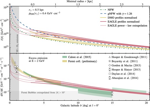
Top panel: the J-factor as a function of galactic latitude b inferred from our four simulated haloes both with (red lines) and without (yellow lines) baryon effects. The green dot–dashed and blue dashed lines correspond to NFW and gNFW with γ = 1.26 profiles, respectively, with a scalelength rs = 20 kpc. To ease comparison, all profiles have been normalized to yield |$\rho _{\rm DM}({r_{\odot }})=0.4\ \rm {GeV}\,\rm {cm}^{-3}$|. The thin lines correspond to power-law extrapolations of our simulated profiles (see text). The scale at the top indicates the minimum radius intersected by a line of sight at the given galactic latitude b. Bottom panel: emission at E = 2 GeV for our haloes assuming the best-fitting particle physics model from Calore et al. (2015b). Data points with error bars show the best-fitting models of Hooper & Goodenough (2011), Boyarsky, Malyshev & Ruchayskiy (2011), Gordon & Macías (2013), Hooper & Slatyer (2013), Daylan et al. (2014) and Abazajian et al. (2014) to the Fermi GeV excess. The green shaded regions indicate the excess emission and its statistical uncertainty for a fixed gNFW profile derived by Calore et al. (2015) and the yellow shaded region indicates the preliminary results of the Fermi-LAT team. The vertical grey shaded region indicates the radial range where uncertainties in the GDE modelling due to π0 emission from H i to H2 regions dominate the foreground templates used in the analysis of the data (adapted from Calore et al. 2015b). Similarly, the shaded region at the bottom indicates the flux intensity of the Fermi bubbles.
4.2 Extrapolation of the profiles towards the centre
As most of the dark matter annihilation signal originates from the inner few hectoparsecs, it is necessary to extrapolate our findings from Section 3.2 to smaller radii. As the annihilation signal increases with the square of the local density, one can ask what the highest density is that can be reached in the inner regions given the constraints on the density and enclosed mass at the smallest converged radius. Assuming that the profile is not hollow and that the logarithmic slope is monotonic, it is straightforward to show that the only asymptotic power law that can be used to extrapolate the profiles from a given radius r towards the centre has a slope γmax = 3(1–4πr3ρ(r)/3M(r)) (Navarro et al. 2010). Setting r to the convergence radius of the haloes, RP03, we obtain slopes in the range γmax = 0.55–1.22 for our four haloes. The J-factors resulting from these extrapolations are shown on Fig. 4 using thin lines. They allow us to set upper bounds on the J-factor for angles b ≲ 3°. Even with this power-law extrapolation, the flux is lower than the gNFW profile with a slope γ = 1.26.
4.3 Gamma-ray flux morphology
In the bottom panel of Fig. 4, we show the emission at E = 2 GeV for our J-factors, assuming the best-fitting particle physics model of Calore et al. (2015).3 For comparison, we show the flux inferred from the GC excess by Hooper & Goodenough (2011), Boyarsky et al. (2011), Gordon & Macías (2013), Hooper & Slatyer (2013), Daylan et al. (2014) and Abazajian et al. (2014) with the error bars indicating the ±1σ statistical error (not shown when smaller than the symbols). The observed intensities were rescaled following the procedure highlighted in Calore et al. (2015b), taking into account the assumed excess profiles. Note that individual measurements are more than 3σ discrepant with each other. The green shaded regions indicate the best-fitting model of Calore et al. (2015). Their model assumed a gNFW profile for the dark matter profile and used 60 GDE templates in their likelihood analysis of 10 regions of interest on the sky located around the GC. The width of the green regions on the figure indicates both the statistical uncertainty and the posterior range of the GDE modelling around the best-fitting gNFW profile. The uncertainty on the slope of the profile is not shown. A similar analysis, performed by Calore et al. (2015b), of the preliminary results of the Fermi collaboration is shown as a yellow shaded region. The grey shaded region on the left of the plot indicates the radial range over which the emission from the ISM gas dominates the GDE models (Calore et al. 2015b). Similarly, the grey shaded region at the bottom of the panel indicates the level of γ-ray flux expected from the extended ‘Fermi bubbles’ (Su, Slatyer & Finkbeiner 2010), thought to be the remnant of past AGN activity. We use the extrapolation, assuming a constant density, to lower latitudes of the flux estimated by Ackermann et al. (2014). The flux originating from the annihilation of dark matter is higher than the contribution of the Fermi bubbles at angles b < 15°, making the radial range 2° < b < 15° ideal for the study of the excess (Calore et al. 2015b). The resolution of our simulations is, hence, well matched to this requirement.
Our simulated profiles (red lines) are in good agreement with the γ-ray data for angles b > 3°. This is expected since over the relevant radial range, the profiles have a similar form to the gNFW profile with asymptotic inner slope, γ = 1.2–1.3, inferred directly from the data (assuming that the emission is due to dark matter annihilation). At smaller angles, three of the four extrapolated profiles give significantly less emission than observed, whilst the fourth is in good agreement with the data. We stress, however, that this extrapolation gives the largest power-law signal at the GC. The predicted emission at b < 2° could be boosted by adjusting the particle physics model but there is a danger that such adjustments could lead to an overprediction of the emission at larger angles.
5 SUMMARY AND CONCLUSION
In this study, we investigated the dark matter density profiles of four MW galaxies simulated using a state-of-the-art hydrodynamics code and subgrid model. We specifically focused on the inner few kiloparsecs of the dark matter distribution in order to refine earlier predictions for the properties of dark matter annihilation emission. The careful treatment of baryons in our simulations allows us to understand and analyse the effects that baryons have on the dark matter distribution. These are not negligible and give rise to haloes whose properties differ significantly from those of the ‘standard halo model’ often used in dark matter detection studies. Whilst our simulations are among the highest resolution examples of their kind currently available, we are only able to establish convergence within a tolerance of 30 per cent across different resolutions over the radial range of interest (Section 3.3). We feel that this level of convergence is sufficient to support our conclusions but higher resolution simulations will be needed to test this supposition.
We can summarize our findings as follows:
As seen in previous simulations (e.g. Dubinski 1994; Abadi et al. 2010; Bryan et al. 2013), the central concentration of baryons significantly reduces the asphericity typical of haloes in dark matter-only simulations. The distribution of dark matter in the inner 500 pc is very close to spherical with axis ratios, b/a > 0.96, in all cases.
There is no detectable offset between the position of the GC and the peak of the dark matter distribution. The largest offset found in our haloes is 45 pc, much smaller than the softening length of the simulations (ϵ = 134 pc).
The condensation of baryons at the halo centre causes the halo to contract slightly. The halo density profiles end up having steeper profiles than NFW in the radial range r = 2-10 kpc.
In the inner 1.5 kpc, which are well resolved in our simulations the dark matter halo density profiles develop significant flattening. This feature is likely to be associated with violent star formation events that take place during the early stages of galaxy formation. It must be borne in mind that effects of this kind are sensitive to the specific subgrid physics model and, at this point, they must not be regarded as a generic prediction of the ΛCDM model.
The predicted dark matter annihilation emission signal is in good agreement with the detection of extended γ-ray emission in excess of the known foregrounds by the Fermi satellite at galactic latitudes, b ≳ 3°, where our haloes are well resolved. A simple extrapolation of the density profiles in our simulations to smaller angles predicts a γ-ray flux significantly lower than is measured, in three of the four cases, suggesting possible contributions from other sources to the excess. In the fourth case, the annihilation signal from the extrapolation is in broad agreement with the reported measurements close to the GC.
The analysis of the Fermi excess has so far been performed assuming a gNFW profile or other parametric profile forms for the dark matter. Future, more precise studies, would benefit from using the more realistic profile shapes derived directly from hydrodynamical simulations. This should help disentangle the signal from dark matter annihilation from the GDE.
This work would have not been possible without Lydia Heck and Peter Draper's technical support and expertise. This work was supported by the Science and Technology Facilities Council (grant number ST/F001166/1); European Research Council (grant numbers GA 267291 ‘Cosmiway’ and GA 278594 ‘GasAroundGalaxies’) and by the Interuniversity Attraction Poles Programme initiated by the Belgian Science Policy Office (AP P7/08 CHARM). RAC is a Royal Society University Research Fellow.
This work used the DiRAC Data Centric system at Durham University, operated by the Institute for Computational Cosmology on behalf of the STFC DiRAC HPC Facility (www.dirac.ac.uk). This equipment was funded by BIS National E-infrastructure capital grant ST/K00042X/1, STFC capital grant ST/H008519/1, and STFC DiRAC Operations grant ST/K003267/1 and Durham University. DiRAC is part of the National E-Infrastructure. We acknowledge PRACE for awarding us access to the Curie machine based in France at TGCC, CEA, Bruyères-le-Châtel.
The thick disc population of MSPs and pulsars are unlikely to contribute more than 10 per cent to the GeV excess (Calore, Di Mauro & Donato 2014).
Note that for simplicity we use units convenient for particle physics applications. Units more friendly to astronomers are recovered using the conversion |$1\ \,{\rm {M}_{\odot }}\,\rm {kpc}^{-3}=3.795 \times 10^{-8}\ \rm {GeV}\,\rm {cm}^{-3}$|.
mχ = 46.6 GeV, |$\langle \sigma v\rangle =1.60\times 10^{-26}\ \rm {cm}^3\ \rm {s}^{-1}$| for a |$b\bar{b}$| final annihilation state.
REFERENCES
APPENDIX A: RESOLUTION TEST FOR ALL HALOES
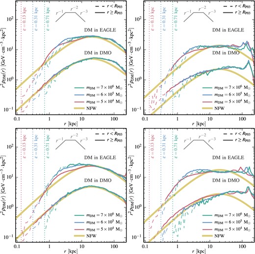
Same as Fig. 3 but for all four haloes considered in this study. The DM density profiles in all four haloes agree to better than 30 per cent at r < 10 kpc.
