


Abstract
We present 237 new spectroscopically confirmed pre-main-sequence K- and M-type stars in the young Upper Scorpius subgroup of the Sco–Cen association, the nearest region of recent massive star formation. Using the Wide-Field Spectrograph at the Australian National University 2.3 m telescope at Siding Spring, we observed 397 kinematically and photometrically selected candidate members of Upper Scorpius, and identified new members by the presence of lithium absorption. The HR-diagram of the new members shows a spread of ages, ranging from ∼3 to 20 Myr, which broadly agrees with the current age estimates of ∼5–10 Myr. We find a significant range of Li 6708 equivalent widths among the members, and a minor dependence of HR-diagram position on the measured equivalent width of the Li 6708 Å line, with members that appear younger having more lithium. This could indicate the presence of either populations of different age, or a spread of ages in Upper Scorpius. We also use Wide-Field Infrared Survey Explorer data to infer circumstellar disc presence in 25 of the members on the basis of infrared excesses, including two candidate transition discs. We find that 11.2 ± 3.4 per cent of the M0–M2 spectral type (0.4–0.8 M⊙) Upper Sco stars display an excess that indicates the presence of a gaseous disc.
1 INTRODUCTION
The Scorpius–Centaurus–Lupus–Crux association (Sco OB2, Sco–Cen) is the nearest location to the Sun with recent high-mass star formation (de Zeeuw et al. 1999). Young OB associations, such as Sco–Cen, provide an incredible laboratory in the form of a primordial group of stars directly after formation, which can be exploited in the study of the output of star formation including searches for young exoplanets. The obvious prerequisite for such study is a level of completeness in the identification of association members that is currently not yet attained in Sco–Cen in any mass regime, other than the most massive B-type stars. Sco–Cen contains approximately 150 B-type stars (Rizzuto, Ireland & Robertson 2011) which have been typically split into three subgroups: Upper Scorpius, Upper Centaurus–Lupus (UCL) and Lower Centaurus–Crux (LCC) with only the B-, A- and F-type membership of Sco–Cen being considered relatively complete, with some 800 members. Even in this high-mass regime, there is expected to be an ∼30 per cent contamination by interlopers in the kinematic membership selections, mainly due to the lack of precision radial velocity measurements for these objects (Rizzuto et al. 2011). Additionally, in light of the upcoming high-precision GAIA proper motions and parallaxes, a well characterized spectroscopically confirmed Sco–Cen membership will be instrumental in illuminating the substructure of the association.
Unfortunately, Sco–Cen is poorly characterized for its proximity, the reason for which is the enormous area of sky the association inhabits at low Galactic latitudes (∼80° × 25° or ∼150 pc × 50 pc). Initial mass function (IMF) extrapolation from the high-mass members implies, with any choice of IMF law, that Sco–Cen is expected to have ∼104 pre-main-sequence (PMS) G-, K- and M-type members, most of which are, as yet, undiscovered. This implies that the vast majority of PMS (<20 Myr) stars in the solar neighbourhood are in Sco–Cen (Preibisch et al. 2002), making Sco–Cen an ideal place to search for young, massive planetary companions. Although some work has been done in illuminating the lower mass population of Sco–Cen (see Preibisch & Mamajek 2008), the late-type membership of Sco–Cen cannot be considered complete in any spectral type or colour range. A more complete picture of the late-type membership of Sco–Cen is the primary requirement for determining the age spread, structure, and star formation history of the association, for illuminating the properties of star formation, and for embarking on further searches for young exoplanets to better define their population statistics.
The age of the Sco–Cen subgroups has been contentious. Upper Scorpius has long been considered to be ∼5 Myr old; however, recent work has shown that it may be as old as 11 Myr (de Geus 1992; Pecaut, Mamajek & Bubar 2012). Similarly, B-, A- and F-type UCL and LCC members have main-sequence turn-off/on ages of ∼16–18 Myr, while studies of the incomplete sample of lithium-rich G-, K- and M-type members show a variety of mass-dependent age estimates. The HR-diagram age for the known K-type stars in UCL and LCC is ∼12 Myr, the few known M-type stars indicate a significantly younger age of ∼4 Myr, most likely due to a bias produced by a magnitude-limited sample, and the G-type members have an age of ∼17 Myr, which is consistent with the more massive stars (Preibisch & Mamajek 2008; Song, Zuckerman & Bessell 2012). There is also a positional trend in the age of the PMS stars of the older subgroups, with stars closer to the Galactic plane appearing significantly younger than objects further north. This is almost certainly the result of as yet undiscovered and unclarified substructure within the older subgroups, which may have a very complex star formation history.
The above is clear motivation for the identification of the full population of the Sco–Cen association, a task that will require significant observational and computational effort to complete. In this paper, we describe a new search for PMS members of the Upper Scorpius region of the Sco–Cen association. We have used statistical methods to select a sample of likely Upper Scorpius members from all-sky data, and have conducted a spectroscopic survey to determine youth and membership in the Sco–Cen association using the Wide-Field Spectrograph (WiFeS) instrument at the Australian National University 2.3 m telescope.
2 SELECTION OF CANDIDATE MEMBERS
We have selected candidate Upper Scorpius members using kinematic and photometric data from UCAC4, 2MASS, USNO-B and APASS (Monet et al. 2003; Skrutskie et al. 2006; Henden et al. 2012; Zacharias et al. 2013). A purely kinematic selection of the low-mass members of Sco–Cen is not sufficient to assign membership to G-, K- and M-type stars because the quality of the astrometric data available would produce an interloper contamination much higher than would be acceptable for future studies using Sco–Cen as an age benchmark. In order to clearly separate young Upper Scorpius members from field stars, spectroscopic follow-up is needed to identify stellar youth indicators. We employed two separate selection methods to prioritize targets based on kinematic and photometric data.
The first selection used was based on the Bayesian Sco–Cen membership selection of Rizzuto et al. (2011), which uses kinematic and spatial information to assign membership probabilities. We further developed this method to apply to K- and M-type stars, in order to properly treat the absence of a parallax measurement. We took the proper motions from the UCAC4 catalogue (Zacharias et al. 2013) and photometry from 2MASS and APASS (Skrutskie et al. 2006; Henden et al. 2012), and used the photometry and a PMS isochrone (Siess, Dufour & Forestini 2000) to estimate each candidate member's distance. We then treated the proper motion and estimated distance together to calculate the membership probability. This selection was magnitude limited, and covered all stars in the UCAC4 catalogue with 10 < V < 16, and comprised of ∼2000 candidate members with membership probability greater than 2 per cent. For a more complete explanation of the Bayesian selection, including information from Rizzuto et al. (2011) and the changes adopted for use with the K- and M-type star data (see Appendix A).
The second selection was based on the selection used for the Coma-Ber cluster in the study of Kraus & Hillenbrand (2007), and was designed to select targets for the Upper Scorpius field of the Kepler K2 campaign. Targets which were both placed above the main sequence based on photometric distance estimates, and had proper motions consistent with Upper Scorpius membership were deemed to be potential members and included in the observing sample. This selection spanned F- to late-M-type stars, with targets falling on Kepler silicon prioritized for spectroscopic follow-up. This selection is considerably more conservative than the Bayesian selection, and includes a much larger number of candidates. Where the two selections overlap, we have >90 per cent of the Bayesian-selected stars included in the sample. Our final, combined sample was then drawn from both of the above selection; we include a candidate in the final target list if it was identified by either method. Fig. 1 displays the proper motions of the selected stars from both samples.
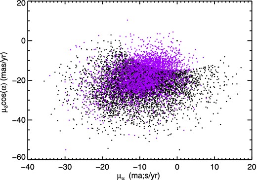
The proper motions of the candidate Upper Scorpius members selected by both the Kraus & Hillenbrand (2007) selection method (black points) and the Bayesian method (purple circles).
In light of the currently ongoing Galactic Archeology Survey, using the HERMES spectrograph on the Anglo-Ausralian Telescope (Zucker et al. 2012), which will obtain high-resolution optical spectra in the coming years for all stars in the Sco–Cen region of sky, down to V = 14, we have decided to primarily observe targets in our sample fainter than this limit. While our selection methods identified candidate Upper Scorpius stars across the entire subgroups (342° < l < 360°, 10° < b < 30°) in our observations, we strongly favoured candidate members which fell upon the Kepler K2 field 2 detector regions, which covers the majority of the centre of Upper Scorpius with rectangular windows. As such, the spatial distribution of this sample will not reflect the true substructure of Upper Scorpius. We observed all the targets in our K2 sample with Kepler-interpolated V magnitudes of (∼13.5 < Vjk < 15), as well as some further brighter targets. In total, we obtained optical spectra for 397 candidate Upper Scorpius K- and M-type stars. The full list of observed candidate targets, including both those stars determined to be members and non-members, can be found in Table 1, along with proper motions, computed Bayesian membership probability, integration time and signal-to-noise ratio (SNR) in the continuum near Hα.
Summary of WiFeS observations of candidate Upper Scorpius members; the V magnitude provided is either taken from APASS, where available, or interpolated from J and K according to the Kepler K2 instructions. The full table is provided in the online material.
| R.A. | Decl. | V | K | μα | μδ | T | |||||
|---|---|---|---|---|---|---|---|---|---|---|---|
| (J2000.0) | (J2000.0) | MJD | (mag) | (mag) | (mas) | (mas) | Source | Pmem | (s) | SNR | M? |
| 15 39 06.96 | −26 46 32.1 | 56462 | 12.5 | 8.7 | −35.3 | −41.7 | a | 31 | 90 | 131 | Y |
| 15 37 42.74 | −25 26 15.8 | 56462 | 13.5 | 9.7 | −14.6 | −26.7 | a | 85 | 90 | 80 | |
| 15 35 32.30 | −25 37 14.1 | 56462 | 11.7 | 8.4 | −9.0 | −22.9 | a | 69 | 90 | 116 | |
| 15 41 31.21 | −25 20 36.3 | 56462 | 10.0 | 7.2 | −16.9 | −28.7 | a | 86 | 90 | 151 | Y |
3 SPECTROSCOPY WITH WiFeS
The WiFeS instrument on the Australian National University 2.3 m telescope is an integral field, or imaging, spectrograph, which provides a spectrum for a number of spatial pixels across the field of view using an image slicing configuration. The field of view of the instrument is 38 arcsec × 25 arcsec, and is made up of 25 slitlets which are each 1 arcsec in width, and 38 arcsec in length. The slitlets feed two 4096 × 4096 pixel detectors, one for the blue part of the spectrum and the other for the red, providing a total wavelength coverage of 330–900 μm, which is dependent on the specific gratings used for the spectroscopy. Each 15 μm pixel corresponds to 1 arcsec × 0.5 arcsec on sky.
There are a number of gratings offered to observers for use with WiFeS. For identification of Upper Scorpius members, we required intermediate-resolution spectra of our candidate members, with a minimum resolution of ∼3000 at the Li 6708 Å line, and so selected the R7000 grating for the red arm and the B3000 grating for the blue arm, which was used solely for spectral typing. This provided λ/Δλ ∼ 7000 spectra covering the lithium 6708 Å and Hα spectroscopic youth indicators. A dichroic, which splits the red and blue light on to the two arms of the detector, can be positioned either at 4800 or 5600 Å. For the first three successful observing nights, we use the dichroic at 4800 Å which produced a single joined spectrum from 3600 to 7000 Å. For the remaining seven nights, we position the dichroic at 5600 Å which produces two separate spectra, with the blue arm covering 3600 to 4800 Å and the red arm covering 5300 to 7000 Å. This change was made to accommodate poor weather backup programmes being simultaneously carried out, which will be the subject of future publications. To properly identify members, we required a 3σ-detection of a 0.1-Å equivalent-width (EW) Li line, which corresponds to an SNR of at least 30 per pixel. In order to achieve this, we took exposures of 5 min for R = 13 stars (approximately type M3 in Upper Scorpius), and binned by 2 pixels in the y-axis, to create 1 arcsec × 1 arcsec spatial pixels and reduce overheads. With overheads, we were able to observe 10 targets an hour in bright time, or ∼80–90 targets per completely clear night.
In total, we obtained 18 nights of time using WiFeS, split over 2013 and 2014; however, the majority of the 2013 nights were unusable due to weather. Our first two observing runs, in 2013 June, and 2014 April yielded one half-night of observations each, and our final observing run yielded seven partially clear nights. During our first two nights, we positioned the dichroic at 5500 Å, and during the 2014 June observing run, positioned the dichroic at 4600 Å, which provides more of the red arm, because this mode was deemed better for obtaining radial velocities of B-, A- and F-type Sco–Cen stars, which we observed as backup targets during poor weather, and will be the subject of a future publication.
4 DATA REDUCTION
The raw WiFeS data were initially reduced with a pre-existing python data reduction software package called the ‘wifes pypeline’, which was provided to WiFeS observers (Childress et al. 2014). The purpose of the software is to transform the CCD image, which consists of a linear spectrum for each spatial pixel of the WiFeS field of view, into a data cube. This involves bias subtraction, flat-fielding, bad pixel and cosmic ray removal, sky subtraction, wavelength calibration, flux calibration, reformatting into the cube structure and interpolation across each pixel to produce a single wavelength scale for the entire image. On each night, we observed at least one flux standard from Bessell (1999), which are included in the data reduction pipeline as flux calibrator objects. Once this process is complete, the user is left with a single cube for each object observed, with dimensions 25 arcsec × 38 arcsec × 3650 wavelength units. For the grating resolutions and angles used in our observations, we obtained spectral coverage from 3200 to 5500 Å in increments of 1.3 Å in the blue arm, and 5400–7000 Å in increments of 0.78 Å in the red arm.
Following the standard WiFeS reduction procedure, we continued with a further custom reduction, the aim of which was to measure the centroid position of the target object in each wavelength, such that the presence of Hα-emitting low-mass stellar companions, outflows, and Hα-bright planetary mass companion could be detected by the measurement of a wavelength-dependent centroid shift. This consisted of determining a best-fitting point spread function (PSF) model for the spatial image in a clean section of the spectrum, and then measuring the centroid shift of this PSF at each wavelength along the spectrum. An additional benefit of this is a more accurate sky subtraction, and an integrated spectrum of each object, which can be used to measure EWs of key spectral lines. The results of the centroid measurements and any detected companions will be reported in a further publication.
We first cut out a 10 arcsec × 10 arcsec wide window (10 × 10 pixels), centred on the target. The vast majority of the stellar flux is contained within the central 3 arcsec by 3 arcsec region of the windowed image, and so the adopted width of 10 arcsec allows a clear region of background around the target; Fig. 2(b) provides an illustration of the data. We then fit a Moffat PSF (Racine 1996) to a region of the spectral continuum which does not include any spectral features, but is close to the Hα line. This region consisted of 400 spectral units, spanning 6368–6544 Å. Fig. 2(a) displays the spectral region used for the initial PSF fit, as well as the Hα and Li 6708 Å lines for one target in our sample, 1RXS J153910.3-264633, which shows strong indications of youth.
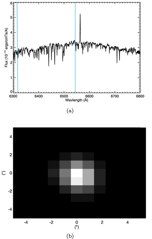
(a) Example spectrum for object 1RXS J153910.3-264633, a high priority target in our observation sample, which shows signs of youth such as Hα emission and Li 6708 Å absorption. The region of the continuum used for the initial PSF fitting is bounded by blue lines. (b) Spatial image created for 1RXS J153910.3-264633 by adding the images at each wavelength of the PSF fitting region of the continuum.
We found that β = 4, a value which describes most telescope PSFs, yielded the closest fit to our data. We also attempted to fit a Gaussian profile to the spatial images, in the same format as the Moffat profile described in equation (1); however, the Gaussian model produced consistently poorer fits to the data than the Moffat model, particularly in the wings of the PSF, with typical values of |$\chi ^2_r\sim 4$| for the Gaussian model fit and |$\chi ^2_r\sim 2$| for the Moffat model. On the basis of the goodness of fit difference, we adopted the Moffat model exclusively in our analysis. For each target observed, we used the continuum spectral region between 6368 and 6544 Å to determine the parameters of the Moffat PSF that most closely reproduced the spatial images. We then fixed the half-width parameters in each dimension, and fit our PSF model to each individual wavelength element image along the spectrum to determine S, F and the centroid position for each wavelength. This process provides two useful characteristics, the first of which is the integrated spectrum (F) of the target (see Fig. 3), with the sky component (S) subtracted out. Using the cleaned output spectra, we then computed EWs of both the Li 6708 Å and Hα lines for each observed star. The second useful characteristic is the centroid position of the star image at each wavelength interval in the spectrum. This can be used to detect accreting stellar and substellar companions by the measurement of a centroid shift in the Hα line image. An analysis of the centroid positions will be presented in a future publication.
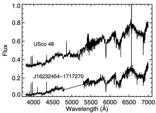
The full WiFeS-integrated spectrum produced by first processing with the wifes pypeline, and then our spectroastrometric analysis for the stars USco 48, a known member of the Upper Scorpius subgroup, and 2MASS J16232454-1717270, high-probability candidate, and a new member in identified in our survey. The USco 48 spectrum is an example of the data from the 4800-Å dichroic setup, and the 2MASS J16232454-1717270 spectrum an example of the 5600-Å dichroic setup.
4.1 Spectral typing
We spectral type the reduced spectra created by the centroid-fitting procedure using spectral template libraries as reference. It is also important to incorporate extinction into the spectral-typing procedure for Upper Scorpius, given the typical values of 0.5 < AV < 2.0. If an extinction correction is omitted, spectral typing will produce systematically later spectral types for the members. A combination of two template libraries was chosen for the spectral typing, with spectral types earlier than M0 taken from the Pickles (1998) spectral template library, and the M-type templates taken from the more recent Bochanski et al. (2007).
To carry out the spectral typing, we first computed reduced χ2 values for each data spectrum on a two-dimensional grid of interpolated template spectra and extinction, with spacing of half a spectral subtype and 0.1 mag in E(B − V). This was done by first interpolating the template spectra on to the wavelength scale of the data, and then applying the particular amount of extinction according to the Savage & Mathis (1979) extinction law. We also removed the Hα region in the data spectra, because the prevalence of significantly larger Hα emission in young stars will not be adequately reproduced by the templates. The spectral type–extinction point on the grid with the smallest reduced χ2 was then used as a starting point for least-squared fitting with the idl fitting package mpfit. The fitting procedure used the same methodology as the grid calculations, with the addition of interpolation between template spectra to produce spectral subtype models for use in the fitting.
We find the limiting factor in spectral typing our young Sco–Cen stars to be the fact that the spectral template libraries are built from field stars, and so are not ideal for fitting young, active stars. Hence, while we typically have spectral type fits better than half a spectral subtype, we report spectral types to the nearest half subtype, and values of AV with typical uncertainties of 0.2 mag.
5 THE NEW MEMBERS
Table 2 lists both the Li 6708 Å and Hα EWs, and the estimated spectral types and extinction for the new Upper Sco members, and Fig. 4 shows the spatial positions of the new members. We have defined a star as an Upper Scorpius member if the measured equivalent width of the Li 6708 Å line was more than 1σ above 0.1 Å. While this Li threshold is low, it is significantly larger than the field Li absorption, and is in general keeping with previous surveys. The use of this threshold is further justified given the effects of episodic accretion on Li depletion in the latest models (Baraffe & Chabrier 2010). In general, the vast majority of the identified members have Li 6708 Å EW significantly larger than 0.2 Å and so are bona fide young stars. In total, we identify 257 stars as members based on their Li 6708 Å absorption, 237 of which are new.
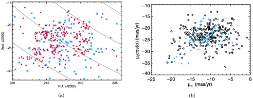
(a) On-sky positions of the new members (red circles), relative to the B-, A- and F-type members (blue stars) from Rizzuto et al. (2011). Lines of constant Galactic latitude are shown in grey in steps of 10°, the centre line is b = 20°. Note that the apparent substructure seen in the new members is artificially created because we strongly prioritized the Kepler K2 Field 2 detector regions in our survey. (b) The proper motions of the new members (black) and the Hipparcos Upper Scorpius members from Rizzuto et al. (2011, blue crosses), the typical proper motion uncertainty for our new members is 2–3 mas yr−1. There is one new member off-scale at (−35.3, −41.7) mas yr−1. Our new members occupy the same region of proper motion space as the established high-mass members.
Properties of the Upper Scorpius members identified in our survey. The first column lists our adopted naming system for these new members and the second column lists the 2MASS designation for each of our targets. We also list the fitted spectral type and visual extinction, and the EWs of the Li 6708 Å and Hα lines [EW(Li) and EW(Hα)]. The full table is provided in the online material.
| R.A. | Decl. | EW(Li) | σEW(Li) | EW(Hα) | |$\sigma _{\mathrm{EW(H_{\alpha })}}$| | AV | |||
|---|---|---|---|---|---|---|---|---|---|
| Name | 2MASS | (J2000.0) | (J2000.0) | (Å) | (Å) | (Å) | (Å) | SpT | (mag) |
| RIK-1 | J15390696-2646320 | 15 39 06.96 | −26 46 32.1 | 0.46 | 0.02 | −1.22 | 0.03 | M0.5 | 0.2 |
| RIK-2 | J15413121-2520363 | 15 41 31.21 | −25 20 36.3 | 0.40 | 0.01 | −2.70 | 0.04 | K2.5 | 0.1 |
| RIK-3 | J15422621-2247458 | 15 42 26.21 | −22 47 46.0 | 0.46 | 0.04 | −3.08 | 0.07 | M1.5 | 0.3 |
| RIK-4 | J15450970-2512430 | 15 45 09.71 | −25 12 43.0 | 0.61 | 0.02 | −2.02 | 0.04 | M1.5 | 0.4 |
The proper motions of the new members, which were calculated from various all-sky catalogues, or taken from the UCAC4 catalogue are shown in Fig. 4(b). The members have proper motions that overlap the Upper Scorpius B-, A- and F-type members proper motions (blue crosses), although a significantly large spread is seen. This is consistent with the average uncertainty of ∼2–3 mas yr−1 for the K- and M-type proper motions.
Fig. 5(a) displays the lithium EWs for the identified members as a function of spectral type. The majority of our members are M type, and we see a sequence of EW with a peak at spectral type M0, and a systematically smaller EW in the M2–M3 range compared to earlier or later M-type members. This is expected as the mid-M range is modelled to show faster lithium depletion time-scale (D'Antona & Mazzitelli 1994).
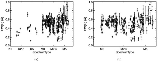
EW(Li) for the new members. The left-hand panel shows the full K- to late-M-spread, while the right-hand panel focusses on the M-type range, which shows the largest spread in EW(Li) for a given spectral type.
Interestingly, we also observe a clear spread in the EW of the Lithium 6708 Å line. Fig. 5(b) shows the just the M0 to M5 spectral type range. At each spectral type, we see a typical spread of ∼0.4 Å in Li EW, and a median uncertainty in the EW measurements of ∼0.03 Å. This implies an ∼10σ spread in EW(Li) at each spectral type. Whether or not this spread is caused by an age spread in Upper Scorpius is difficult to determine: we have examined the behaviour of EW(Li) as a function of spatial position, both in equatorial and Galactic coordinate frames and found no significant trend. We note that a similar spread of EW(Li) for M-type Upper Scorpius members was observed by Preibisch, Guenther & Zinnecker (2001). Given the lack of correlation with spatial position, if the EW(Li) spread is caused by an age spread among the members, then the different age populations are overlapping spatially and may not be resolvable without submilliarcsecond parallaxes.
In Fig. 6, we display the measured Hα EWs for the members. The majority of the PMS members show some level, of Hα emission, with a clear sequence of increasing emission with spectral type. In combination with the presence of lithium, this is a further indicator of the youth of these objects. Of our 257 members, ∼95 per cent show Hα emission with (1 Å<EW(Hα)<10 Å), and only 11 of the members do not show emission in Hα. All of these 11 members without Hα emission are earlier than M0 spectral type. There are also 35 non-members with Hα emission. Given the values of EW(Hα) for the M-type members we have identified, the majority of them appear to be weak-lined T-Tauri stars and ∼10 per cent are Classical T-Tauri stars (CTTS) with EW(Hα) > 10 Å. This proportion agrees with previous studies of Upper Scorpius members (Walter et al. 1994; Preibisch & Zinnecker 1999; Preibisch et al. 2001), which find a CTTS fraction of between 4 and 10 per cent for K- and M-type Upper-Scorpius stars.
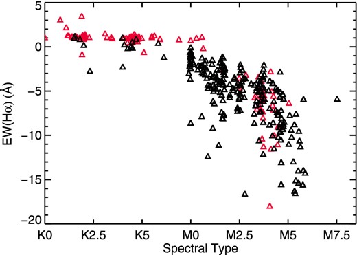
EW(Hα) for the new members (black) and the non-members (red). The members follow a clear sequence with Hα increasing with spectral type. In the K spectral types, we see that non-members show Hα absorption which is generally stronger than that seen in the members, some of which show weak emission.
6 THE EFFICIENCY OF THE BAYESIAN SELECTION ALGORITHM
The selection methods we have used to create our target list provide a significant improvement of member detection rate when compared to what can be achieved from simple colour–magnitude cuts. We see a large overall identification rate of ∼65 per cent for our sample of observed stars. Using the membership probabilities computed for the stars we have observed, we expected that 73 ± 7 per cent of the observed stars would be members, which agrees with the observed members fraction of 68 per cent. We also find that as a function of computed membership probability, the fraction of members identified among the sample behaves as expected. Fig. 7 displayed the membership fraction as a function of probability.
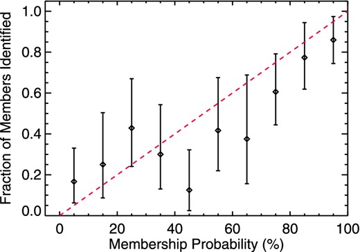
Fraction of stars identified as members plotted against membership probability computed with our Bayesian selection algorithm. The red line represents the ideal fraction of detected members. We see a very close agreement between the computed membership probability and the fraction of stars which were confirmed as members.
Given that our probabilities have been empirically verified to provide a reasonable picture of Upper Scorpius membership, we can derive an estimate for the expected number of M-type members in the subgroup by summation of the probabilities. We find that the total expected number of Upper Scorpius members in the ∼0.2 to 1.0 M⊙ range, or late-K to ∼M5 spectral type range, is ∼2100 ± 100 members. This agrees with IMF estimates which indicate that there are ∼1900 members with masses smaller than 0.6 M⊙ in Upper Scorpius (Preibisch et al. 2002).
7 THE HR-DIAGRAM OF THE MEMBERS
With the spectral types and extinctions we have determined for the members using the Bochanski et al. (2007) and Pickles (1998) spectral libraries, we can place them on an HR-diagram in the model parameter space. There is significant variability in synthesized photometry between different models for PMS stars, making comparison in the colour–magnitude space difficult. Furthermore, the most reliable magnitudes for M-type stars are the near-IR 2MASS photometry, which show minimal variation in the M-type regime where the PMS is near vertical. Instead, we use the spectral types and the empirical temperature scale and J-band bolometric corrections for 5–30 Myr stars produced by Pecaut & Mamajek (2013) and we further correct for extinction using our fitted values of AV from the spectral-typing process, and the Savage & Mathis (1979) extinction law. The resulting HR-diagram can be seen in Fig. 8. We have also superimposed five BT-Settl (Allard, Homeier & Freytag 2011) isochrones of ages 1, 3, 5, 10 and 20 Myr on to the HR-diagram at the typical Upper Scorpius distance of 140 pc (Rizzuto et al. 2011). These particular models were chosen because they were used by Pecaut & Mamajek (2013) in the generation of their temperature scale, and so any relative systematic differences between the models and the temperature scale will most likely be minimized.
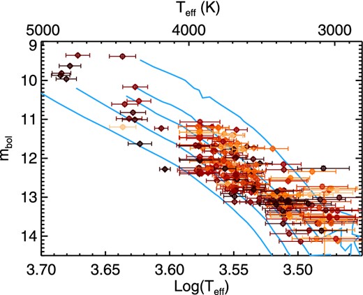
HR-diagram for the Upper Scorpius members we have identified, with bolometric corrections and effective temperatures taken from the Pecaut & Mamajek (2013) young star temperature–colour scale. The blue lines are the BT-Settl isochrones (Allard et al. 2011) of ages 1, 3, 5, 10 and 20 Myr placed at the typical distance to Upper Scorpius of 140 pc. The colour of each point indicates the measured EW(Li) for the star, with darker colour indicating a lower EW(Li). The colour range spans 0.3 <EW(Li)<0.7 linearly, with values outside this range set to the corresponding extreme colour. The uncertainties are determined by the accuracy of our spectral typing methods, which is typical half a spectral subtype.
Upon initial inspection, it appears that for a given temperature range, the Upper Scorpius members inhabit a significant spread of bolometric magnitudes. This is most likely highly dominated by the distance spread of the Upper Scorpius subgroup, which has members at distances between 100 and 200 pc, corresponding to a spread in bolometric magnitude of ∼1.5 mag between the nearest and furthers reaches of Upper Scorpius. Using the distance distribution of the Rizzuto et al. (2011) high-mass membership for Upper Scorpius, we find that the expected spread in bolometric magnitude due to distance which encompasses 68 per cent of members is approximately +0.33 and −0.54 magnitudes. Similarly, unresolved multiple systems can bias the sample towards appearing younger by an increase in bolometric magnitude of up to ∼0.7 mag for individual stars.
In the later spectral types, beyond log Teft = 3.52 we also begin to see the effects of the magnitude limit of our survey, which operated primarily in the range 13.5 < V < 15 and so only the brightest, and hence nearest and potentially youngest late-M-type members in our original target list were identified, although significant Li depletion at these temperatures is not expected to occur until ages beyond 50 Myr. Even with distance spread blurring the PMS in Upper Scorpius, we can see that most of the members appear to be centred around the 5–10 Myr age range in the earlier M-type members.
We have also indicated the measured EW(Li) values for the members on the HR-diagram as a colour gradient, with darker colour indicating a smaller EW(Li). The scale encompasses a range of 0.3 < EW(Li) < 0.7 Å, with values outside this range set to the corresponding extreme colour. There is a marginal positional dependence of HR-diagram position with EW(Li): we see that, in particular for the earlier M-type members, the larger values of EW(Li) (light orange) are more clustered around the 3–5 Myr position, while the smaller values of EW(Li) (dark red) are clustered closer to 5–10 Myr. This could indicate the presence of a spread of ages, or populations of different age in the Upper Scorpius subgroup.
There is some other evidence of different age populations in the Upper Scorpius subgroup: the existence of very young B-type stars, such as τ-Sco, and ω-Sco which have well-measured temperatures and luminosities that indicate an age of ∼2–5 Myr (Simón-Díaz et al. 2006) support a young population in Upper Scorpius. The B0.5 binary star δ-Sco is also likely to be quite young (∼5 Myr; Code et al. 1976). Pecaut et al. (2012) place it on the HR-diagram at an age of ∼10 Myr; however, due to the rapid rotation and possible oblate spheroid nature of the primary, the photometric prescriptions for determining the effective temperature and reddening of the primary used by Pecaut et al. (2012) are likely to fail for this object. The spectral type is more consistent with a temperature of ∼30 000 K. Additionally, the presence of other evolved B-type stars is evidence for an older population (Pecaut et al. 2012). Furthermore, the recent age estimate of 13 Myr for the F-type members of Upper Scorpius by Pecaut et al. (2012) further supports an older population in the subgroup. If the HR-diagram position on EW(Li) that we observe among our members is real than this also supports multiple age population in Upper Scorpius.
8 Disc CANDIDATES
We have also obtained the Wide-Field Infrared Survey Explorer (WISE) infrared photometry (Wright et al. 2010), from the ALLWISE version of the catalogue, for the observed candidate members in order to determine the prevalence of circumstellar discs among our new members. The identification of new populations of stars bearing discs is valuable because it provides extension to the current samples used in the study of disc property measurements and disc evolution. The AllWISE catalogue provides photometry in four bands W1, W2, W3 and W4, with effective wavelengths of 3, 4.5, 12 and 22 μm, respectively. The W2 and W3 photometry is effective for tracing the presence of an inner disc, while excess in the W4 band photometry can indicate the presence of a colder, outer disc or transitional disc.
We queried the ALLWISE catalogue for the positions of the 397 stars we observed from our sample, including 237 new members, with a search radius of 5 arcsec. The search returned 395 matches with varying levels of photometric quality. We then placed each star on three spectral type colour diagrams incorporating 2MASS (Skrutskie et al. 2006) K-band photometry, these were K−W2, K−W3, and K−W4. Past studies have used both K, and W1 as the base photometry for building colour–colour diagrams (Carpenter et al. 2006, 2009; Luhman et al. 2010; Luhman & Mamajek 2012; Rizzuto, Ireland & Zucker 2012). Typically, the presence of a disc within ∼3 au of a host star increases the brightness in the IR wavelengths, with ∼5 μm being the approximate wavelength where the disc dominates in brightness. Both the W1 and K magnitudes are long enough such that reddening is not a significant issue, but also shorter than the expected point of disc domination. We found that examining the WISE bands relative to the K magnitude produced a better separation of disc-bearing stars from photospheric emission, and so we report the analysis in terms of this methodology.
Fig. 9 displays the three spectral type colour diagrams. We excluded any WISE photometry in a given band that was flagged as having an SNR of <4, as a non-detection, or flagged as being contaminated by any type of image artefact in the catalogue. This resulted in the exclusion of 56, 10 and 312 objects in the W2, W3, and W4 bands, respectively. The primary source of the exclusions for the W4 band was non-detection or low signal to noise at 22 μm, and most of the exclusions in the W2 and W3 bands were due to contamination by image artefacts. To reduce contamination by extended sources, we also excluded any object flagged as being nearby a known extended source or with significantly poor photometry fits, there were eight such objects. The WISE band images for these stars were then inspected visually to gauge the extent of contamination. We found the three of the objects were not significantly affected by the nearby extended source, and so included them in the analysis. After excluding these objects, we were left with 333, 379 and 77 objects with photometry of sufficient quality in the W2, W3 and W4 bands, respectively.
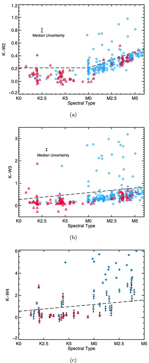
Near IR and WISE band colour–colour diagrams for both the newly identified members (blue diamonds) and non-members (red triangles) from our spectroscopic survey for (J − K, K − W2), (J − K, K − W3) and (J − K, K − W4). We have omitted objects in each WISE band that were flagged as having poor or contaminated photometry in the catalogue. The dashed lines indicate the position of the upper boundary of the photospheric sequence. If a star is above this threshold, we designate it as displaying an excess in the particular band.
Due to the age of Upper Scorpius of ∼10 Myr, the majority of members no longer possess a disc, providing sufficient numbers of stars to clearly identify photospheric emission. Hence, the photosphere colour can be determined from the clustered sequence in the spectral type colour diagrams. We fit a straight line in the K−W3 and K−W4 WISE band colours, and a disjointed line in K−W2, and then place a boundary where the photospheric sequence ends. For K−W3, the boundary line is given by the points (K0,0.27) and (M5,0.8) and for K−W4 the points (K0,0.56) and (M5,1.6). The sloped part of the boundary line for K−W2 is defined by the points (M0,0.21) and (M5,0.46), and the flat section by K−W2 = 0.21, for spectral types earlier than M0. These boundaries are shown as black lines in Fig. 9. Stars with colour redder than these boundaries we deem to display an excess in the particular WISE band. Upon inspection, we find that our placement of the end of the photospheric sequence is closely consistent with that of Luhman & Mamajek (2012). In the K−W4 colour, we find that for stars of spectral type later than ∼M2, the photospheric emission in W4 is undetectable by WISE.
For those stars which displayed excesses in any combination of WISE bands, we visually inspected the images to exclude the possibility that the excesses could have been caused by the presence of close companions or nebulosity. We also found that in a few cases background structure in the W4 image could cause the appearance of an excess, although this effect was largely mitigated by our signal-to-noise cut-off. We rejected 23 of the excess detections after inspection, 12 of which were caused by background structure or nearby nebulosity, and 11 of which were due to blending with nearby stars. We further excluded any object which shows an excess in only the K−W2 colour as likely being produced by unresolved multiplicity. After these rejections, 27 stars remained with reliable excess detections. Additionally, a single object, 2MASS J16194711-2203112, displayed an excess in K−W3, but had a W4 detection with signal-to-noise of 3.5. Upon inspection of the corresponding W4 band image, we included it as exhibiting an excess in K−W4.
We can classify the disc types by the amount of excess displayed in different colours compared to the photosphere. We adopt disc-type criteria in the E(K−W4), E(K−W3) space consistent with those described in Luhman et al. (2010) and Luhman & Mamajek (2012), which identify four different categories of disc: full or primordial discs, transition discs, evolved discs and debris or evolved transition discs. Primordial or full discs exhibit strong emission across the entire IR spectral range. Transition discs are structurally different in that they have a significant cleared inner hole, which is visible as a weaker emission at the shorter IR wavelengths, but still relatively bright in the longer IR wavelengths. Evolved discs do not show a gap in IR emission, but have started to become thinned and appear fainter at all IR wavelengths than unevolved full discs, with a steady decline in IR excess with age (Carpenter et al. 2009). Debris disc and evolved transition disc have similar IR SED's, showing only weak excesses at the longer IR wavelengths. Fig. 10(b) show both E(K−W4) and E(K−W3) for the stars identified as having displaying an excess. The lines in Fig. 10(b) bound the different regions populated by the various disc types. We classify all objects with excesses in W3 and W4 beneath the dashed line to be debris or evolved transition discs candidates, and the objects above the solid line to be full discs. Stars with excess between these two lines we classify as evolved disc candidates. Finally, we identify the two objects with a large W4 excess, but W3 excesses too small to be classified as full discs, as transition disc candidates. Table 3 lists the excess status for the stars with detected excesses.
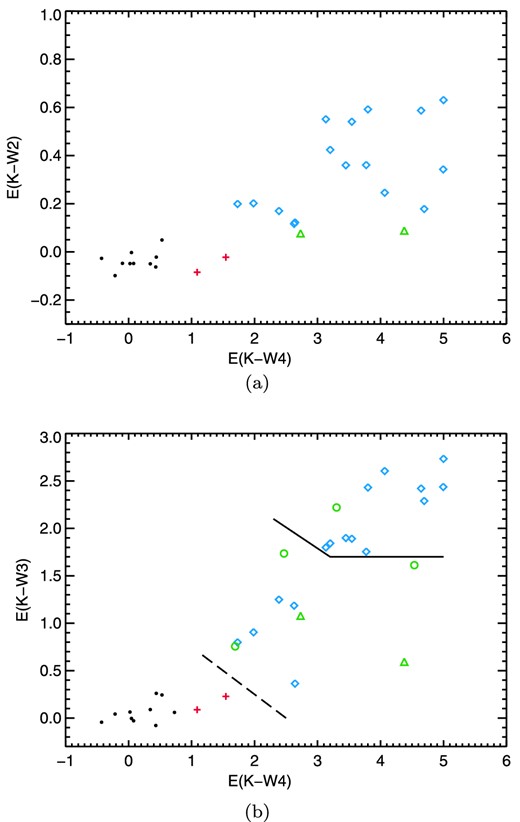
Excesses in K−W2 versus K−W4 and K−W3 versus K−W4 for the members observed in our survey. The plots includes members without excess (black circles), with excesses in W2, W3 and W4 (blue diamonds), with excesses in the two longest WISE bands with and without reliable W2 photometry (green triangles and circles, respectively), and members with an excess in only the W4 band (red plusses). We also include three members with just W3 excesses, which were detected in W4, but without excesses which clearly sit above the discless sequence (purple squares). The black lines indicate adopted boundaries for different disc classifications.
List of stars in our sample with observed IR excesses in the WISE bands. (M) indicates the membership status of the star, (E) list the detection of IR excesses in the three WISE bands, (D) labels the candidate disc classification where F, E, T and D/ET mean full, evolved, transition, and debris or evolved transition, respectively. The final three columns list the availability of photometry in the three longest WISE bands. The question mark (?) indicates the star HD-145778, which is likely to be an F-type members of Upper Scorpius.
| R.A. | Decl. | |||||||
|---|---|---|---|---|---|---|---|---|
| 2MASS | (J2000.0) | (J2000.0) | M | E | D | W2 | W3 | W4 |
| 15581270-2328364 | 15 58 12.70 | −23 28 36.4 | Y | XXE | D/ET | 7.97 | 7.88 | 6.72 |
| 15573430-2321123 | 15 57 34.31 | −23 21 12.3 | Y | EEE | E | 8.67 | 8.30 | 5.58 |
| 16052157-1821412 | 16 05 21.57 | −18 21 41.2 | Y | XEE | T | 7.24 | 6.36 | 3.16 |
| 16064385-1908056 | 16 06 43.86 | −19 08 05.5 | Y | EEE | E | 8.86 | 8.11 | 6.79 |
| 16064794-1841437 | 16 06 47.94 | −18 41 43.8 | Y | XEE | T | 8.75 | 8.10 | 3.93 |
| 16120668-3010270 | 16 12 06.68 | −30 10 27.1 | Y | EEE | F | 8.81 | 6.58 | 3.60 |
| 16134781-2747340 | 16 13 47.82 | −27 47 34.0 | Y? | XEE | E | 7.93 | 7.81 | 7.04 |
| 15594426-2029232 | 15 59 44.27 | −20 29 23.4 | Y | EEE | F | 9.59 | 8.07 | 6.12 |
| 16120505-2043404 | 16 12 05.05 | −20 43 40.5 | Y | EEE | E | 8.71 | 7.50 | 5.93 |
| 16112601-2631558 | 16 11 26.03 | −26 31 55.9 | Y | XEE | E | 9.24 | 8.12 | 5.98 |
| 16093164-2229224 | 16 09 31.66 | −22 29 22.4 | Y | EEE | F | 8.65 | 6.17 | 4.23 |
| 16252883-2607538 | 16 25 28.81 | −26 07 53.8 | Y | XXE | D/ET | 9.61 | 9.24 | 7.43 |
| 16333496-1832540 | 16 33 34.97 | −18 32 53.9 | Y | XEE | E | 9.81 | 9.21 | 7.72 |
| 16023587-2320170 | 16 02 35.89 | −23 20 17.1 | Y | XEE | E | 9.79 | 8.31 | 7.41 |
| 16011398-2516281 | 16 01 13.99 | −25 16 28.2 | Y | EEE | E | 9.97 | 8.79 | 6.81 |
| 16132190-2136136 | 16 13 21.91 | −21 36 13.7 | Y | EEE | F | 9.40 | 7.88 | 5.41 |
| 16194711-2203112 | 16 19 47.12 | −22 03 11.2 | Y | XEX | E | 10.13 | 9.24 | |
| 16041893-2430392 | 16 04 18.93 | −24 30 39.3 | Y | EEE | F | 8.23 | 6.57 | 4.52 |
| 16100501-2132318 | 16 10 05.02 | −21 32 31.9 | Y | EEE | F | 8.23 | 6.25 | 3.64 |
| 16200616-2212385 | 16 20 06.16 | −22 12 38.5 | Y | XEE | E | 10.12 | 8.48 | 7.20 |
| 15564244-2039339 | 15 56 42.45 | −20 39 34.2 | Y | EEE | F | 9.79 | 7.57 | 4.63 |
| 16271273-2504017 | 16 27 12.74 | −25 04 01.8 | Y | EEE | F | 8.64 | 7.25 | 5.48 |
| 15583620-1946135 | 15 58 36.20 | −19 46 13.5 | Y | EEE | F | 9.74 | 7.53 | 4.70 |
| 16012902-2509069 | 16 01 29.03 | −25 09 06.9 | Y | EEE | F | 9.19 | 7.24 | 5.34 |
| 16071403-1702425 | 16 07 14.02 | −17 02 42.7 | Y | XEE | F | 10.25 | 8.10 | 6.47 |
| 16145244-2513523 | 16 14 52.41 | −25 13 52.4 | Y | EEE | E | 9.95 | 9.13 | 7.52 |
| 16153220-2010236 | 16 15 32.20 | −20 10 23.7 | Y | EEE | F | 8.16 | 6.68 | 4.57 |
In total, we identify 26 of the Upper Scorpius members as displaying a disc-indicating excess with spectral types later than K0, and one star without significant lithium absorption that also displays an excess. This latter object is an F4.5 spectral type object,, HD-145778, with EW(Li) = 0.09 ± 0.2. The presence of some lithium absorption, combined with the disc presence mean that this object can be considered to be a member of Upper Scorpius. We have included it as a member at the end of Table 2. HD-145778 is not in this HIPPARCOS catalogue (Perryman et al. 1997), potentially explaining why it was not included in past memberships.
Due to the WISE detection limit in the W4 band, we are almost certainly not able to identify the vast majority of the evolved transitional and debris discs, which show only a small colour excess in K−W4. Indeed, we only detect two such discs in our sample, one of which, USco 41, was previously identified with Spitzer photometry (Carpenter et al. 2009), when significantly more are expected from previous statistics (Carpenter et al. 2009; Luhman & Mamajek 2012). Furthermore, it is likely that a number of evolved discs around stars of spectral type later than ∼M3 are not detected here. For this reason, it is difficult to meaningfully estimate the disc or excess fraction for our entire sample. In the M0 to M2 spectral type range, where we expect the majority of the full, evolved and transitional discs to be detectable by WISE, we have 11 discs, six of which are full, four evolved and one transitional. Excluding all those members flagged for extended emission, confusion with image artefacts, or unreliable excesses, we find and excess fraction of 11.2 ± 3.4 per cent. Carpenter et al. (2009) found a primordial disc fraction for M-type Upper Scorpius members of ∼17 per cent, and Luhman & Mamajek (2012) find excess fractions of 12 and 21 per cent for K-type and M0- to M4-type members, respectively. Given the strong increase in excess fraction towards the late-M-type members and the potential for some missed evolved discs due to the WISE detection limits, we find that our excess fraction estimate is consistent with these past results.
9 CONCLUSIONS
We have conducted a spectroscopic survey of 397 candidate Upper Scorpius association K- and M-type members chosen through statistical methods, and revealed 237 new PMS members among the sample based on the presence of Li absorption. We also identify 25 members in our sample with WISE near-infrared excesses indicative of the presence of a circumstellar disc, and classify these discs on the basis of their colour excess in different WISE bands. We find that the members show a significant spread in EW(Li), and upon placing the members on an HR-diagram, we find that there is a potential age spread, with a small correlation between EW(Li) and HR-diagram position. This could indicate the presence of a distribution of ages, or multiple populations of different age in Upper Scorpius.
We thank Michael Childress for assistance and explanation of the data reduction packaged used to complete this work. We also thank the anonymous referee for helpful suggestions which improved the paper.
REFERENCES
APPENDIX A: BAYESIAN SELECTION OF CANDIDATE PMS UPPER SCORPIUS STARS
For the kinematic models, we employ the same linear models in Galactic longitude for the group model, and the Galactic thin disc model of Robin et al. (2003), as were used in Rizzuto et al. (2011).
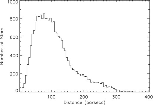
Field photometric distance distribution, showing features of the input catalogue magnitude and colour cuts, and the isochrone used in estimation of the distances.
SUPPORTING INFORMATION
Additional Supporting Information may be found in the online version of this article:
Table 1. Summary of WiFeS observations of candidate Upper Scorpius members; the V magnitude provided is either taken from APASS, where available, or interpolated from J and K according to the Kepler K2 instructions.
Table 2. Properties of the Upper Scorpius members identified in our survey. The first column lists our adopted naming system for these new members and the second column lists the 2MASS designation for each of our targets. We also list the fitted spectral type and visual extinction, and the EWs of the Li 6708 Å and Hα lines [EW(Li) and EW(Hα)] (Supplementary Data).
Please note: Oxford University Press are not responsible for the content or functionality of any supporting materials supplied by the authors. Any queries (other than missing material) should be directed to the corresponding author for the article.
