


Abstract
In this work, we analyse the Lyman α forest in cosmological hydrodynamical simulations of Chameleon-type f(R)-gravity with the goal to assess whether the impact of such models is detectable in absorption line statistics. We carry out a set of hydrodynamical simulations with the cosmological simulation code mg-gadget, including star formation and cooling effects, and create synthetic Lyman α absorption spectra from the simulation outputs. We statistically compare simulations with f(R) and ordinary general relativity, focusing on flux probability distribution functions and flux power-spectra, an analysis of the column density and linewidth distributions, as well as the matter power spectrum. We find that the influence of f(R)-gravity on the Lyman α forest is rather small. Even models with strong modifications of gravity, like |$|\bar{f}_{R0}| = 10^{-4}$|, do not change the statistical Lyman α properties by more than 10 per cent. The column density and linewidth distributions are hardly affected at all. It is therefore not possible to get competitive constraints on the background field fR using current observational data. An improved understanding of systematics in the observations and a more accurate modelling of the baryonic/radiative physics would be required to allow this in the future. The impact of f(R) on the matter power spectrum in our results is consistent with previous works.
1 INTRODUCTION
Theoretically explaining the late time accelerated expansion of the Universe is one of the biggest challenges in modern cosmology. In the standard model of cosmology, the Λ cold dark matter (ΛCDM) model, the cosmological constant Λ is responsible for the acceleration. While the ΛCDM model is quite successful in explaining many aspects of cosmic structure formation, it also features some problems, one of them being the lack of a natural explanation for Λ. This encourages the search for alternative theories.
In general, the models attempting to provide a theoretical explanation for the accelerated expansion can be divided into two main classes. The first class, which also includes ΛCDM, contains so-called dark energy models. These models add a new type of ‘matter’ to the energy–momentum tensor of general relativity (GR). If this type of matter is described by an equation of state with a negative effective pressure, it can drive the accelerated expansion.
The second class are the so-called modified gravity models. To explain the accelerated expansion, they modify the gravitational interaction. In other words: while the dark energy models change the right-hand side of Einstein's equation, the modified gravity models modify its left-hand side.
In this work, we consider f(R)-gravity, which can be viewed as a member of the second class. The modification to gravity is carried out by adding a scalar function of the Ricci-scalar R to the action of GR. Because GR is well tested in our local environment, particularly in the Solar system, modified gravity theories typically share the need for some screening mechanism which suppresses the modification of GR in high-density environments. Examples for such screening mechanisms are the Chameleon (Khoury & Weltman 2004), the Symmetron (Hinterbichler & Khoury 2010), the Vainshtein (Vainshtein 1972) or the Dilaton (Gasperini, Piazza & Veneziano 2002) mechanism. In f(R)-gravity, the screening mechanism is determined by the particular choice of f(R). We here consider a model proposed by Hu & Sawicki (2007), which gives rise to a Chameleon mechanism.
Previous simulation works on Chameleon-type f(R)-gravity mainly employed collisionless simulations, analysing, e.g. halo mass functions (e.g. Schmidt et al. 2009; Ferraro, Schmidt & Hu 2011; Li & Hu 2011; Zhao, Li & Koyama 2011), matter power spectra (e.g. Oyaizu 2008; Li et al. 2012, 2013; Puchwein, Baldi & Springel 2013; Llinares, Mota & Winther 2014), density profiles (Lombriser et al. 2012a; Corbett Moran, Teyssier & Li 2014), cluster concentrations (Lombriser et al. 2012b), the integrated Sachs–Wolfe effect (Cai et al. 2014), redshift space distortions (Jennings et al. 2012), velocity dispersions (Schmidt 2010; Lam et al. 2012; Lombriser et al. 2012b; Arnold, Puchwein & Springel 2014), the impact of screening on the fifth force in galaxy clusters (Corbett Moran et al. 2014) and galaxy populations which were followed with a semi-analytical model (Fontanot et al. 2013). Using hydrodynamical simulations instead, we studied in previous work (Arnold et al. 2014) the temperature of the intracluster medium and different mass measures of galaxy clusters.
In this work, we will for the first time extend the analysis of hydrodynamical f(R) modified gravity simulations to the statistical properties of the Lyman α forest. Employing the modified gravity simulation code mg-gadget, we carry out simulations to redshift z = 2, given that most Lyman α data lie at redshifts z ∼ 2–4. Creating synthetic Lyman α absorption spectra from the simulation outputs, we present an analysis of flux probability distribution functions (PDFs), flux power spectra, line shape statistics, as well as of the matter power spectrum for both f(R)-gravity and an ordinary ΛCDM model. We particularly focus on the relative differences between these two cosmogonies and compare our results to observations.
This paper is structured as follows. In Section 2, we give a brief summary of the particular parametrization of f(R) we adopt, whereas Section 3 describes the simulation set we have carried out. In Section 4, we present our main results. Finally, we give a summary and our conclusions in Section 5.
2 f(R)-GRAVITY
3 SIMULATIONS AND METHODS
Modelling the statistical properties of the Lyman α forest requires a cosmological simulation code which is capable of accounting for a variety of gas physics, including photoheating, radiative cooling and star formation. For f(R)-gravity, the fifth force influence has to be computed in addition. In this work, we use the modified gravity simulation code Modified-Gravity-gadget (mg-gadget; Puchwein et al. 2013), which is an extension of p-gadget3, which in turn is an advanced version of gadget2 (Springel 2005). Featuring the gas-physics modules of p-gadget3 as well as a modified gravity solver, mg-gadget offers the possibility to analyse the Lyman α forest in the Hu & Sawicki (2007) model of f(R)-gravity, including non-linear effects caused by the Chameleon mechanism.
mg-gadget solves the f(R)-equations as follows (for full details of the code functionality; see Puchwein et al. 2013): First, equation (3) is solved using an iterative Newton–Gauss–Seidel relaxation scheme. The iterations are carried out on an adaptively refining mesh so that an increased resolution is available in high-density regions without causing a great loss of performance. Solving for fR directly could lead to positive values for f(R) due to the finite iteration step-size. Because this would immediately stop the simulations, the code solves for |$u \equiv \ln (f_{\rm R} /\bar{f}_{\rm R}(a))$| instead (following Oyaizu 2008), and then calculates f from u. This iterative scheme is well suited for the highly non-linear behaviour of fR.
For a reliable analysis of f(R)'s impact on the Lyman α forest it is necessary to run simulations in both modified gravity and ΛCDM using identical initial conditions. We do so by carrying out hydrodynamical simulations using 2 × 5123 particles (5123 each gas and dark matter) in a 60 h−1 Mpc box for |$|\bar{f}_{R0}| = 10^{-5}$| and GR. To explore the parameter space at a coarse level, we also did a set of smaller box simulations at the same mass resolution, but using 2 × 1283 particles in a 15 h−1 Mpc box for |$|\bar{f}_{R0}| = 10^{-4}$|, 10−5 and GR. Our set of cosmological parameters is |$\Omega _{\rm m} = 0.305, \Omega _\Lambda = 0.695, \Omega _{\rm b} = 0.048$| and H0 = 0.679, consistent with cosmic microwave background constraints.
To extract the statistical properties of the Lyman α forest, synthetic absorption spectra were calculated at different redshifts. Using the output of the hydrodynamical simulations, we randomly select 5000 lines of sight (LOS), each intersecting the simulation box parallel to one of the three coordinate axes. Dividing each line into 2048 pixels, the density of the neutral hydrogen, the gas temperature and the neutral gas weighted velocity fields of the gas are computed along the LOS. For this computation, we consider all SPH particles whose smoothing length is intersected by the sight-line. With the bulk flow velocities and temperatures along the LOS in hand, we then account for kinematic Doppler shifts and thermal broadening of the absorption lines, which are themselves calculated from the neutral hydrogen density. As final output, the code creates for each LOS a file with optical depth τ as a function of distance along the LOS. This output can be converted into a transmitted flux F = e−τ.
In the simulations, mg-gadget uses a tabulated UV-background1 which allows the calculation of gas temperatures and ionization fractions assuming ionization equilibrium. The results might however not fit the mean Lyman α flux transmission actually seen in the observational data. In order to compare the mock spectra to observations more faithfully, it is therefore necessary to tune the mean transmitted flux to the corresponding value obtained in the observations. We perform this rescaling of the optical depths, which is a standard procedure in theoretical studies of the Lyman α forest, in our post-processing of the LOS data.
4 RESULTS
In analysing the synthetic Lyman α absorption spectra, we first consider the PDF of the transmitted flux fraction in the 60 h−1 Mpc box simulations for both |$|\bar{f}_{R0}| = 10^{-5}$| and ΛCDM. Fig. 1 shows these PDFs at redshifts z = 2, 2.5 and 3 (left-hand panels), as well as the relative differences between the two cosmological models (right-hand panels). The mean transmitted flux fraction is tuned in this plot to the observational values of Kim et al. (2007). We also show this data in the panels on the left-hand side and its relative errors on the right-hand side, for reference. In addition, the results of Calura et al. (2012) are shown for redshift z = 3. In both observations metal lines were excised, in the latter also Lyman-limit systems (LLS). The mean transmission measured by Calura et al. (2012) is consistent with the one of Kim et al. (2007). We can thus compare to the same theoretical prediction.
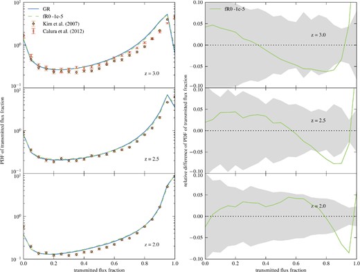
Left-hand panel: PDF of the transmitted flux fraction for different redshifts for ΛCDM and |$|\bar{f}_{R0}| = 10^{-5}$|, using the results of the large simulation boxes. The dots with error bars show the data of Kim et al. (2007). For z = 3, the observational results of Calura et al. (2012) are shown in addition (we plot the ‘no metals, no LLS’ values of this work here). Right-hand panel: relative difference of the PDFs on the left-hand side. The shaded regions show the 1σ relative errors of the observational results of Kim et al. (2007). The mean transmission is tuned to the values of this work in both panels.
Comparing the absolute values, it is obvious that, despite the tuning to the same effective |$\bar{\tau }$|, the simulation results do not match the observations particularly well. Especially at redshift z = 3, the gap between the simulation results of both f(R)-gravity and GR and the observational values of Kim et al. (2007) is much larger than the error bars. At intermediate fluxes, the Calura et al. (2012) results are much closer to the simulations. Nevertheless, the differences at large transmitted flux fractions clearly exceed the 3σ observational error. Considering the panels for redshift z = 2 and 2.5, the discrepancies between simulations and the observational data are smaller, but in certain regimes still larger than 3σ. These differences might have their origin in the still uncertain systematic errors of observations (like e.g. in the continuum placement) and simulations, in an underestimate of the statistical errors (Rollinde et al. 2013) or in an unaccounted heating of the very low density intergalactic medium (Bolton et al. 2008; Viel, Bolton & Haehnelt 2009) by radiative transfer (McQuinn et al. 2009; Compostella, Cantalupo & Porciani 2013) and non-ionization-equilibrium (Puchwein et al. 2014) effects or, as recently suggested, by TeV blazars (Broderick, Chang & Pfrommer 2012; Puchwein et al. 2012).
The difference between |$|\bar{f}_{R0}| = 10^{-5}$| and ΛCDM is much smaller than the difference between the simulation results and the observed values and somewhat smaller than the error bars of the observations. This is even more obvious in the right-hand panels of Fig. 1. Comparing the relative difference in the flux PDF between f(R) and GR, it turns out that the differences between the models are mostly within the observational errors for individual flux bins for all considered redshifts. The overall deviation over many flux bins and redshifts could, however, still be statistically significant if systematic effects were better understood. Given the current uncertainties in Lyman α forest studies and the already very tight constraints on the Hu & Sawicki (2007) model of f(R)-gravity from other observables, it will therefore be hard to get competitive constrains on |$|\bar{f}_{R0}|$| using the flux PDF of the Lyman α forest.
We arrive at a similar conclusion for the Lyman α flux power-spectra obtained for the large simulation box: Fig. 2 shows their absolute value for both f(R)-gravity and a ΛCDM cosmology as well as the relative difference between these models. The theoretical results from our synthetic spectra are again tuned to the mean transmission of Kim et al. (2007). For z = 3, the simulation values are compared to the observational results of McDonald et al. (2006), with the grey shaded area in the relative difference plot indicating their quoted errors.
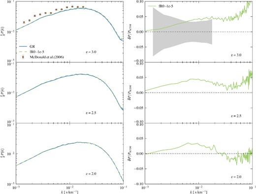
Left-hand panel: flux power spectra for f(R)-gravity and ΛCDM obtained from the 60 h−1 Mpc simulation boxes at different redshifts. The dots with error bars show the results of McDonald et al. (2006). Right-hand panel: relative difference in the flux power spectra shown on the left-hand side. The shaded area represents the relative errors of the McDonald et al. (2006) results at z = 3. The mean transmission is tuned to the values of Kim et al. (2007) for both panels.
As for the flux PDF, the discrepancy between simulations and observations at redshift z = 3 is quite large, in particular much larger than the errors given in McDonald et al. (2006). This might have its origin in systematic uncertainties which are not considered by the error bars. Again, the difference between the two gravitational models is tiny, compared to the difference between observational data and the results from the simulations. Because the difference to GR is again smaller than or comparable to the error bars of the shown observations, we need to conclude that the Lyman α flux power-spectrum is only mildly affected by f(R)-gravity.
This is also particularly evident in the relative difference plots at the right-hand side. The difference in the flux power-spectrum between |$|\bar{f}_{R0}| = 10^{-5}$| and GR is about 5 per cent at maximum, considering redshifts z = 2, 2.5 and 3. Normalizing the results of McDonald et al. (2006) to our ΛCDM outcome, it is obvious that the relative difference between the f(R) simulation results and the fiducial model is consistent with the relative errors quoted for the individual k bins. The overall deviation over many bins and redshifts may be statistically significant. However, systematic effects would need to be better understood to obtain interesting constrains on |$\bar{f}_{R0}$| based on such observations.
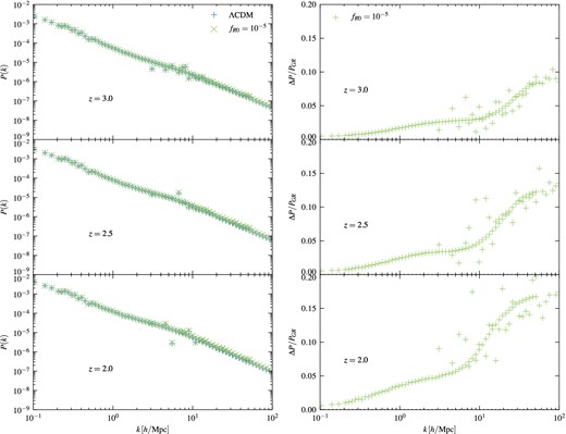
To test if it is at all possible to constrain f(R)-gravity using the Lyman α forest, we also run a set of simulations with smaller box size at equal mass and spatial resolution, for |$|\bar{f}_{R0}| = 10^{-4}, 10^{-5}$| and GR. The power spectra and flux PDFs at redshift z = 3 are shown in Fig. 3. For both power spectra and the PDFs, the results for GR and |$|\bar{f}_{R0}| = 10^{-5}$|, as well as their relative differences, are compatible with the values from the bigger simulation box shown in Figs 1 and 2. One can therefore conclude that the smaller box runs are sufficient for an analysis over the shown range of values. In the |$|\bar{f}_{R0}| = 10^{-4}$| simulations, the flux power spectrum does not fit the observed values of McDonald et al. (2006) despite tuning the mean transmission. As the absolute value of the Lyman α power spectrum is not known with great accuracy, one should not overestimate the, compared to the over gravitational models, smaller difference of the |$|\bar{f}_{R0}| = 10^{-4}$| curve to the observations. Again, normalizing the GR results to the observations, one can compare the observational errors to the differences between f(R) and a ΛCDM universe. At intermediate scales the difference between |$|\bar{f}_{R0}| = 10^{-4}$| and GR is larger than for |$|\bar{f}_{R0}| = 10^{-5}$|. Nevertheless, it does not exceed the 2σ relative error of the observations for individual k bins. Given that |$|\bar{f}_{R0}| = 10^{-4}$| appears already clearly ruled out by other methods (Schmidt et al. 2009; Smith 2009; Lombriser et al. 2012a,b; Dossett, Hu & Parkinson 2014), it does not seem that current Lyman α data can add much new information here.
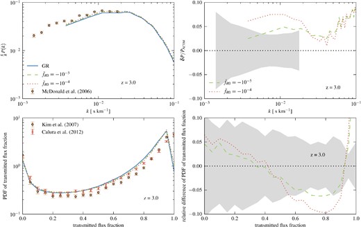
Fig. 3 also shows the PDF of the transmitted flux for the three different gravity models. As for the power spectrum, the |$|\bar{f}_{R0}| = 10^{-4}$| values do not fit the data much better than the other models at z = 3. Comparing relative errors to the difference between the models, we see that the difference between |$|\bar{f}_{R0}| = 10^{-4}$| and GR lies within the 1σ-error region for almost all values. Only between a transmitted flux fraction of 0.6 and 0.9 the difference is larger than 1σ and reaches about 2σ at maximum. The flux PDF does therefore also not seem to be very competitive with current observational data compared to other methods to constrain |$\bar{f}_{R0}$|.
In comparison to other uncertainties in the cosmological model, the impact of f(R)-gravity on Lyman α flux power spectra or PDFs is fairly small, even if one considers quite extreme and already excluded values for |$|\bar{f}_{R0}|$|.
Fig. 4 illustrates how small the modified gravity effect on the Lyman α forest is. It displays the transmitted flux fraction along an arbitrarily selected LOS for f(R) and ΛCDM as a function of distance along this line. The positions of the absorption lines are the same for both models, as identical initial conditions have been used in both simulations. While there appear slight differences in the transmitted flux fractions for the individual absorption lines, no general pattern can be identified from a visual inspection.
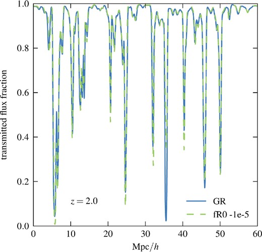
Transmitted flux fraction along an arbitrarily selected LOS at z = 2 for GR and |$|\bar{f}_{R0}| = 10^{-5}$|.
Taking a more systematic approach, we used the code autovp (Davé et al. 1997) to fit Voigt-profiles to the absorption lines of the synthetic spectra. The PDF of the linewidth of the fitted Voigt-profiles is shown in the upper panel of Fig. 5 for all lines with a neutral hydrogen column density |$N_{\rm H\,\small {i}} > 10^{13} \,\rm {cm}^{-2}$| at redshift z = 2. As the lines almost perfectly overlap each other, it is perhaps not surprising that there is no significant difference in the linewidth distributions between f(R)-gravity and a ΛCDM universe. The lower panel of the figure displays the normalized column density PDF of the absorption lines. As for the linewidth, the difference between the curves for |$|\bar{f}_{R0}| = 10^{-5}$| and the ΛCDM model is negligible.
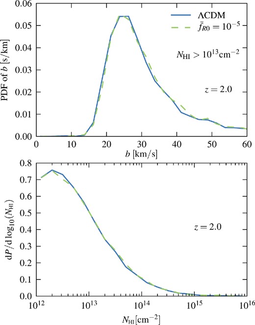
Upper panel: PDF of the linewidths of the Voigt profile fits to the Lyman α absorption lines in the synthetic spectra for all lines with neutral hydrogen column density |$N_{\rm H\,\small {i}} > 10^{13} \,\rm {cm}^{-2}$| at z = 2. Lower panel: normalized PDF of the column density, considering all lines with |$N_{\rm H\,\small {i}} > 10^{12} \rm {cm}^{-2}$| at the same redshift. The spectra for both panels were tuned to the mean transmission of Becker et al. (2013) and were calculated from the 60 h− 1Mpc simulations.
The absolute values of the statistical Lyman α measures depend on the observational value the mean transmitted flux is tuned to. To justify our previous analysis, we briefly show that the relative differences do not depend strongly on the actual value that is adopted. Fig. 6 shows the relative difference in flux PDF and power spectrum between |$|\bar{f}_R| = 10^{-5}$| and GR. Each line in the plot is tuned to a different mean τ, representing the observational data of Becker et al. (2013), Kim et al. (2007) and Faucher-Giguère et al. (2008). The figure shows that neither the relative difference in the power spectra nor the flux PDF do strongly depend on the choice of the tuning value for z = 3. As our analysis confirms, this does also hold for z = 2 and 2.5. One can therefore conclude that the relative differences can be explored safely despite the fact that the absolute values depend on the actual value used for the mean transmission.
Upper panel: relative difference between f(R) and ΛCDM in the Lyman α flux power spectrum; lower panel: relative difference between modified gravity and GR in the PDF of the transmitted flux fraction. For both plots, the values of the mean transmitted flux were tuned either to Kim et al. (2007, blue solid line), Becker et al. (2013, green dashed line), or Faucher-Giguère et al. (2008, brown dotted line), respectively. The results refer to z = 3.
To complement our analysis of the Lyman α forest in the simulations, we also analysed the total matter power spectra at different redshifts. Fig. 7 shows these spectra for |$|\bar{f}_R| = 10^{-5}$| and ΛCDM scenarios at redshifts z = 2, 2.5 and 3, as well as the relative difference between the models. Comparing the power spectrum enhancement to previous works, our results at redshift z = 2 are in good agreement with those of Li et al. (2013). The evolution of the enhancement with time in our simulations is consistent with previous works, too (Li et al. 2013; Winther & Ferreira 2014). This confirms that our f(R) simulations feature an impact of modified gravity at the expected level, even though the effects on the Lyman α forest properties are weak.
Left-hand panel: matter power spectrum for ΛCDM and |$|\bar{f}_{R0}| = 10^{-5}$| at three different redshifts. Right-hand panel: corresponding relative difference in the power spectra (Pf(R) − PGR)/PGR between f(R) and GR.
Considering the relative differences between f(R) and GR in the matter power spectrum, it is very important to note that correct results at small scales and high redshifts can only be obtained from simulations which cover the Chameleon effect in full non-linearity. Linear approximations tend to heavily overestimate the enhancement of the power spectra there as they are missing the suppression of structure formation caused by Chameleon screening (Oyaizu, Lima & Hu 2008; Schmidt et al. 2009; Zhao et al. 2011; Li et al. 2013).
Comparing matter and flux power spectra at the same scale, the relative differences between f(R) and GR are of similar size. The matter power spectra exhibit larger differences at smaller scales. There the Lyman α flux power spectrum becomes, however, degenerate with uncertainties in the temperature of the intergalactic medium. Other gas properties like the temperature of gas in collapsed objects typically show f(R) effects of the order of 30 per cent in the unscreened regime (Arnold et al. 2014). This also illustrates that the impact of f(R)-gravity on the Lyman α forest is rather small in comparison. In order to constrain f(R), it therefore appears more promising to focus on other measures of structure growth rather than the Lyman α forest.
5 SUMMARY AND CONCLUSIONS
In this work, we analysed the statistical properties of the Lyman α forest and the matter power spectra in hydrodynamical cosmological simulations of f(R)-gravity. Our simulations employed the Hu & Sawicki (2007) model and used the modified gravity simulation code mg-gadget. For comparison, we also ran a set of simulations for a ΛCDM universe. Our main findings can be summarized as follows.
The PDF of the transmitted Lyman α flux fraction is only mildly affected by f(R)-gravity. The maximum relative difference between |$|\bar{f}_{R0}| = 10^{-5}$| and GR is of the order of 7 per cent. For |$|\bar{f}_{R0}| = 10^{-4}$|, the difference grows to at most 10 per cent. The simulation results do not fit the observational data of Kim et al. (2007) at all redshifts, regardless of the gravitational model. If the observations are normalized to the GR results from the simulations, the relative differences between the gravitational models do not exceed the 2σ relative error of the observations. For z = 3, the Calura et al. (2012) data match the simulation results at intermediate transmitted flux fractions much better. This highlights that the present observational data is relatively uncertain. At high transmissions there are also significant deviations.
For the flux power spectra, we arrive at similar results. The relative difference between the models reaches at most 5 per cent for |$|\bar{f}_{R0}| = 10^{-5}$| and about 10 per cent for |$|\bar{f}_{R0}| = 10^{-4}$|. Again, the differences to GR for the stronger model are within the 2σ relative error of the observational data (McDonald et al. 2006). Despite tuning the mean transmitted flux to the observational values, the power spectrum at z = 3 does not accurately reproduce the observational data.
There is no significant change in the shapes and abundances of absorption lines in f(R) modified gravity: both the column density and line width distribution functions based on Voigt profile fitting do not exhibit any systematic change.
The relative differences between f(R) and GR in the flux PDF and power spectra do not depend significantly on the observed mean transmission value to which the simulated spectra are scaled. The tuning affects only the absolute values of these statistical Lyman α measures.
The matter power spectrum shows an enhancement in f(R)-gravity which grows with time. The amplitude of the effect and the relative difference to GR is consistent with previous works. These relative changes in the matter power spectrum are of comparable magnitude as the changes in the Lyman α forest flux power spectrum at the same scale. Note, however, that the enhancement of the matter power spectrum continues to grow towards low redshift where it is no longer probed by the Lyman α forest. Also, note that a much stronger influence of f(R) has been found for other gas properties like the gas temperature in collapsed objects in the unscreened regime as has been reported in Arnold et al. (2014).
All in all we arrive at the conclusion that the impact of f(R)-gravity on the Lyman α forest is small. The relative differences in flux PDFs and flux power spectra are only of the order of 5 per cent. Even for likely excluded models, like |$|\bar{f}_{R0}| = 10^{-4}$|, the changes in the statistical Lyman α forest properties do not exceed the relative errors of available observations in individual flux or wavenumber bins. Using the full data over a range of redshifts a detection of modified gravity effects could probably be statistically significant due to its clearly defined signature. However, currently, systematic effects do not seem to be understood at the required level to get competitive constraints in practice. One can therefore conclude that Lyman α forest properties are of limited discriminative power to constrain |$|\bar{f}_{R0}|$| at the moment. The remarkable robustness of the forest statistics has however also advantages. Given that the considered gravitational models have a negligible impact on the Lyman α forest compared to other cosmological and astrophysical uncertainties, it may not be necessary to consider |$|\bar{f}_{R0}|$| as an additional parameter in constraining cosmological parameters based on the Lyman α forest.
CA and VS acknowledge support from the Deutsche Forschungsgemeinschaft (DFG) through Transregio 33, ‘The Dark Universe’. EP would like to thank Martin Haehnelt for helpful discussions and acknowledges support by the FP7 ERC Advanced Grant Emergence-320596.
