


Abstract
Turbulent gas motion inside galaxy clusters provides a non-negligible non-thermal pressure support to the intracluster gas. If not corrected, it leads to a systematic bias in the estimation of cluster masses from X-ray and Sunyaev–Zel'dovich (SZ) observations assuming hydrostatic equilibrium, and affects interpretation of measurements of the SZ power spectrum and observations of cluster outskirts from ongoing and upcoming large cluster surveys. Recently, Shi & Komatsu developed an analytical model for predicting the radius, mass, and redshift dependence of the non-thermal pressure contributed by the kinetic random motions of intracluster gas sourced by the cluster mass growth. In this paper, we compare the predictions of this analytical model to a state-of-the-art cosmological hydrodynamics simulation. As different mass growth histories result in different non-thermal pressure, we perform the comparison on 65 simulated galaxy clusters on a cluster-by-cluster basis. We find an excellent agreement between the modelled and simulated non-thermal pressure profiles. Our results open up the possibility of using the analytical model to correct the systematic bias in the mass estimation of galaxy clusters. We also discuss tests of the physical picture underlying the evolution of intracluster non-thermal gas motions, as well as a way to further improve the analytical modelling, which may help achieve a unified understanding of non-thermal phenomena in galaxy clusters.
1 INTRODUCTION
Precise mass determinations of galaxy clusters are crucial for their cosmological applications. We usually assume hydrostatic equilibrium between the pressure gradient and the gravitational force on the intracluster gas when determining masses from X-ray and Sunyaev–Zel'dovich (SZ) observations. These observations, however, typically measure only the thermal pressure of the gas. Non-thermal pressure, if neglected, introduces a bias in the hydrostatic mass estimation (HSE mass bias). This would, in turn, bias the cosmological constraint from the cluster mass function and the SZ power spectrum, and affect the interpretation of observations of cluster outskirts from ongoing and upcoming large cluster surveys.
Observationally, the HSE mass bias manifests itself as a systematic difference between the X-ray (or SZ) derived mass and the lensing mass of up to 30 per cent (Allen 1998; Mahdavi et al. 2008; Richard et al. 2010; Zhang et al. 2010; von der Linden et al. 2014, but see also non-detections, e.g. Israel et al. 2014). Hydrodynamics numerical simulations of intracluster gas using both grid-based (Iapichino & Niemeyer 2008; Lau, Kravtsov & Nagai 2009; Vazza et al. 2009; Iapichino et al. 2011; Nelson et al. 2014a; Nelson, Lau & Nagai 2014b) and particle-based (Dolag et al. 2005; Vazza et al. 2006; Battaglia et al. 2012) methods have found that the intracluster gas motions generated in the structure formation process contributes significantly to the non-thermal pressure. These alone lead to an HSE mass bias comparable to that found from observations (Rasia et al. 2006, 2012; Nagai, Vikhlinin & Kravtsov 2007; Piffaretti & Valdarnini 2008; Lau et al. 2009; Meneghetti et al. 2010; Nelson et al. 2012). In addition to the structure formation process, turbulent gas motions can be generated in the cluster outskirts by the magnetothermal instability (Parrish et al. 2012; McCourt, Quataert & Parrish 2013), and in the cluster core-by-core sloshing and energy injection from black holes and stars. Magnetic fields and cosmic rays can also potentially contribute to the non-thermal pressure. Residual acceleration of gas, apart from the non-thermal pressure, introduces an additional source of deviation from the hydrostatic equilibrium (Lau, Nagai & Nelson 2013; Suto et al. 2013; Nelson et al. 2014a). We refer to e.g. Shi & Komatsu (2014) for a discussion of these sources, and focus, in the following, on the pressure support from the intracluster gas motions generated during structure formation.
Due to the high Reynold number associated with typical intracluster gas motions, the intracluster gas flow is highly turbulent. Nevertheless, since the turbulence cascade time-scale on galaxy-cluster-size scales can be comparable to the Hubble time, the existence of large-scale coherent motions is expected. Current hydrodynamic simulations cannot yet achieve the high Reynold number characteristic of true turbulence. Still, according to the physical scale of the resolved motions, it is possible to distinguish motions that appear random or coherent on a certain scale and refer to them as ‘turbulence’ and ‘bulk motions’, respectively. When estimating the non-thermal pressure and the HSE mass bias, however, it is not necessary to distinguish ‘turbulence’ and ‘bulk motions’, as both of them contribute in the same way (Lau et al. 2013). In the following, we follow Shi & Komatsu (2014) and refer to the non-thermal random motions in the diffuse intracluster gas as ‘turbulence’ or ‘turbulent gas motions’. Note that the gas motions associated with self-gravitating substructures, on the other hand, do not contribute to the HSE mass bias in general.
Several observations have provided indirect evidence for the intracluster gas motions: measurements of the magnetic field fluctuations in diffuse cluster radio sources (Murgia et al. 2004; Vogt & Enßlin 2005; Bonafede et al. 2010; Vacca et al. 2010), X-ray surface brightness fluctuations or pressure fluctuations inferred from X-ray maps (Schuecker et al. 2004; Churazov et al. 2012; Simionescu et al. 2012), and the non-detection of resonant scattering effects in the X-ray spectra (Churazov et al. 2004). Future observations of the X-ray emission lines are considered as the most promising method to measure turbulence velocities directly (Sunyaev, Norman & Bryan 2003; Shang & Oh 2012; Zhuravleva et al. 2012), and so far the method has already provided a few upper limits in the cluster cores (Sanders, Fabian & Smith 2011; Sanders & Fabian 2013). Whereas these observations greatly contribute to our understanding of the non-thermal phenomena in the intracluster gas, it is hard to use them to estimate the turbulence pressure accurately. Moreover, these observations are mostly limited to nearby clusters or the inner regions with high surface brightness (see Nagai et al. 2013 for an estimation of the detectability of intracluster gas motions by the upcoming Astro-H mission).
On the other hand, the mass estimates require an accurate determination of the non-thermal pressure in the outskirts of clusters where most of the mass resides. Therefore, the amplitude of intracluster turbulence pressure in the outskirts has to be derived theoretically from the existing knowledge of the injection and dissipation of intracluster turbulence.
One way to estimate the turbulence pressure is to measure it from cosmological hydrodynamics simulations. However, since a large, high-precision light-cone hydrodynamics simulation is still too expensive to carry out, it is desirable to have an analytical model that can predict the turbulence pressure, either alone or combined with dark matter only N-body simulations. More importantly, an analytical model is based on physical understandings. Thus, by comparing the predictions drawn from an analytical model to simulations and observations, the physical understandings can be tested and improved, forming a healthy feedback loop.
To this end, Shi & Komatsu (2014, hereafter SK14) developed an analytical model for computing the time evolution of the intracluster turbulence pressure. The model is based on a physical picture of turbulence injection during hierarchical cluster mass assembly, and turbulence dissipation with a time-scale determined by the turnover time of the largest turbulence eddies. In this paper, we shall compare the turbulence pressure predicted by this analytical model to that measured in a state-of-art cosmological hydrodynamics simulation. This comparison will test the validity of the analytical model as well as some aspects of the underlying physical picture.
The rest of the paper is organized as follows. In Section 2, we introduce the simulation and the cluster sample used for the comparison. In Section 3, we demonstrate how to apply the analytical model to the simulation data. In Section 4, we present and discuss the results. The underlying physical picture of turbulence injection and dissipation, as well as how to test them more thoroughly, are discussed in Section 5. We conclude in Section 6.
2 SIMULATION AND CLUSTER SAMPLE
We compare the SK14 model with the outputs of the Omega500 simulation (Nelson et al. 2014a), a large cosmological Eulerian simulation performed with the Adaptive Refinement Tree N-body+gas-dynamics code (Kravtsov 1999; Kravtsov, Klypin & Hoffman 2002; Rudd, Zentner & Kravtsov 2008). In order to achieve the dynamic ranges necessary to resolve the cores of haloes, adaptive refinement in space and time and non-adaptive refinement in mass (Klypin et al. 2001) are used. The simulation has a comoving box length of 500 h−1 Mpc and a maximum comoving spatial resolution of 3.8 h−1 kpc, and is performed in a flat Λ cold dark matter(ΛCDM) model with the WMAP five-year cosmological parameters (Komatsu et al. 2009). For consistency with the physics included in the analytical model, the simulation we use does not include radiative cooling or feedback. See Nelson et al. (2014b) for the implications of neglecting these additional physics in simulations.
We select a mass-limited sample of 65 galaxy clusters at z = 0 from the simulation. Its mass distribution is shown in Fig. 1. We measure one-dimensional profiles of various quantities such as the density and pressure at 25 snapshots between z = 0 and z = 1.5. See Nelson et al. (2014a) and Nelson et al. (2014b, hereafter NLN14) for more information on the simulation and the cluster sample.
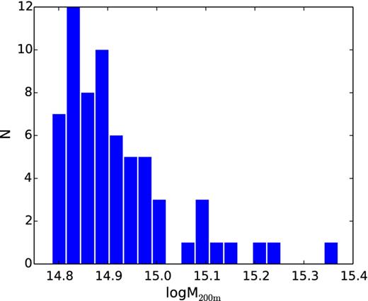
Distribution of cluster masses at z = 0 in the mass-limited sample of simulated galaxy clusters.
Fig. 2 shows the mass accretion histories of the cluster sample. Each of the 65 clusters is assigned a colour depending on their final mass at z = 0. The mass, M200 m, is defined as the mass enclosed within the radius, r200 m, within which the average matter density equals 200 times the mean mass density of the universe. The dashed lines in Fig. 2 show the analytical mean halo mass accretion histories of Zhao et al. (2009) for four representative halo masses. We find that the mass accretion histories of the simulated clusters largely agree with that predicted by Zhao et al. (2009), despite that the most massive clusters in the sample show slightly slower mass accretion histories than the prediction of Zhao et al. (2009). This suggests that the few most massive clusters in the simulated cluster sample can be slightly more relaxed than the cosmic average. We do not expect this to affect generality of our results.
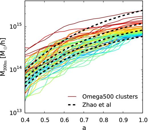
Mass accretion histories of the mass-limited sample of 65 clusters from the Omega500 simulation. Each solid line shows the mass accretion history of one simulated cluster, colour-coded according to its mass at z = 0 (a = 1 where a is the scalefactor). We also show the mean halo mass accretion histories of four different halo masses computed using the Zhao et al. (2009) method (black dashed lines).
3 ANALYTICAL MODEL OF NON-THERMAL PRESSURE
3.1 The model
We need |$\sigma ^2_{\rm tot}$| and td to solve equation (). These quantities are, to first order, dictated by the gravitational potential. The essential input knowledge is then how the gravitational potential deepens with time, or simply the mass accretion history. Different clusters have different mass accretion histories; thus, to compare the model predictions with the simulated clusters on a cluster-by-cluster basis, we take |$\sigma ^2_{\rm tot}$| and td directly from the simulation outputs of individual clusters.
We measure the turbulence velocity dispersion, σnth, in each radial shell as the rms velocity after subtracting the mean velocity of the shell with respect to the centre-of-mass velocity of the total mass interior to this radial shell (NLN14). In Appendix A, we will explain and discuss our procedure of measuring σnth in detail. We then compute the total velocity dispersion squared, |$\sigma ^2_{\rm tot}$|, according to equation (2),1 and compute the non-thermal pressure fraction, fnth, as their ratio, i.e. |$f_{\rm nth} \equiv {\sigma ^2_{\rm nth}}/{\sigma ^2_{\rm tot}}$|. Since fnth is typically much smaller than unity, |$\sigma ^2_{\rm tot}$| is mainly contributed by the thermal velocity dispersion and can be regarded, to the first order, as being proportional to the gas temperature.
3.2 Smoothing the source term
As a cluster grows in mass, its σtot generally increases, suggesting a positive source term in the right-hand side of equation (1). For the simulated clusters, however, the σtot at each Eulerian radius may also decrease due to local inhomogeneities. As an example, in Fig. 3 we show σtot at a few radial bins of one cluster as a function of the scalefactor of the universe. The selected cluster has a mass and an accretion history both close to the median of the mass-limited cluster sample. Some wiggles exist in σtot, which propagate from small to large radii. They likely share the same origin with the peaks in the hydrostatic mass estimates in fig. 2 of Nelson et al. (2012), and correspond to outwardly moving merger shocks that sweep across the cluster region in a time of 1–2 Gyr (see Appendix B).
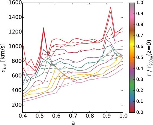
Growth of σtot as a function of the scalefactor of the universe in one representative cluster with a typical mass and accretion history. Each solid line shows σtot measured in the simulation at a certain Eulerian radius indicated by the colour bar. The dashed lines are the smoothed σtot growth curves used in the modelling.
The analytical model does not intend to capture such transient phenomena, but rather their long-term effect on the intracluster medium. Therefore, we smooth these wiggles to reduce their numerical effect. We do so by choosing the points from each simulated σtot(a) curve which have a smaller value than all the points to the right of this curve (at a larger a), and fit linearly between these chosen points. We then use the resulting monotonously increasing σtot(a) (dashed lines in Fig. 3) in the modelling. We note that this smoothing is only performed for the source term in the analytical model, but not in any simulation data used for the comparison. Radial bins that happen to be at the disturbed state (corresponding to the peak of the wiggles) at the time of the comparison would explain part of the scatter in the comparison.
3.3 Initial condition
In SK14, we have argued that, as long as the initial time is chosen to be early enough, the choice of the value of fnth at the initial time does not affect the final value of fnth. In the inner region of the cluster, this is because the short turbulence dissipation time drives fnth quickly to its limiting value determined by the ratio of td and the cluster mass growth time-scale (see section 3.2 of SK14). In the cluster outskirts, the turbulence pressure does accumulate throughout time, but the growth is significant after the region enters the virial radius of the cluster, which occurs only at late times.
In this paper, the initial time is chosen at z = 1.5, which is early enough for the above arguments to hold to a high degree of accuracy for studying cluster profiles at z = 0. Thus, for convenience and consistency, we choose the initial condition to be fnth = 0 for all clusters at z = 1.5. Another option, namely using the values of fnth measured from the simulation at z = 1.5, can provide a more precise initial condition, but only for regions inside clusters which are dynamically relaxed at that time. We have compared the fnth values at z = 0 using this initial condition with those using the default initial condition. The difference is negligible inside r200 m.
4 RESULTS: MODEL VERSUS SIMULATION
We shall limit the comparison between the model predictions and the simulation outputs to (0.1–1)r200 m. We restrict the study to r < r200 m (about 1.3rvir at z = 0 and rvir at z = 1 in a standard ΛCDM cosmology for cluster-mass objects) to avoid the region where there is significant gas infall. We also avoid the cluster core region (r < 0.1r200 m) because of both theoretical and numerical difficulties there, such as the uncertainty on the feedback effect of the central AGNs, the disagreement of numerical methods on gas thermodynamical quantities in the core region, and the ambiguity in the choice of the cluster centre and its consequence on the projected one-dimensional profiles. Outside the core region the observational measurement of the velocity field becomes exceedingly difficult, implying that the observational test of the model may be restricted to a few nearby systems even with upcoming instruments. This, on the other hand, emphasizes the importance of analytical understanding of the non-thermal pressure, as well as the comparison of analytical models and numerical simulations.
We choose β = 1 and η = 0.7 as the preferred value (SK14). Effects of varying β and η will be presented in Section 4.2. All comparison will be performed on the cluster sample at z = 0.
4.1 Non-thermal pressure fraction
We show the comparison of the modelled and simulated non-thermal fraction profiles of six clusters in Fig. 4. The clusters are selected such that their masses spread over the full range. For all clusters shown, there is a clear trend of fnth increasing with radius in the simulated profiles. This trend is a natural consequence of an increasing turbulence dissipation time at larger radii, and is well reproduced by the modelled profiles. On the other hand, the values of the non-thermal fraction at the same radius scaled by r200 m vary by a factor of a few among the clusters. This distinctive difference in the fnth values is also well reproduced by the modelled profiles.
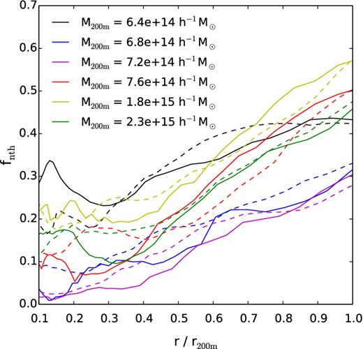
Comparison of modelled (solid lines) and simulated (dashed lines) fnth profiles of individual clusters. Profiles of six typical clusters with a spectrum of different masses at z = 0 are shown. The radius is scaled with r200 m, which has a value of about 2.3 Mpc h−1 for a cluster with the median mass of the sample.
The mean fnth profiles of the whole sample are shown in Fig. 5. The solid and the dashed lines are the modelled and simulated profiles, respectively. Not only does the mean agree, but also the magnitude of the scatter (shown by the shaded regions) agrees.
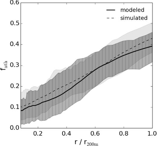
Non-thermal fraction profile of the mass-limited sample. The solid line and the hatched shaded region are the mean and the 16/84 percentile of the modelled profiles; the dashed line and the unhatched shaded region are those of the simulated profiles.
Fig. 6 shows a more quantitative comparison of the modelled and simulated fnth values. Each data point here shows the modelled versus simulated fnth values in one logarithmic radial bin of one cluster in the sample. Larger fnth values are found at larger radii, as shown by the colour-coding. To guide the eye, we group the data points into bins according to their modelled fnth values, and mark the median simulated fnth value of each group with a black point whose x-position indicates the centre of the bin. The associated error bar shows the 1σ scatter of the simulated fnth distribution. We find an excellent agreement between the modelled and simulated fnth.
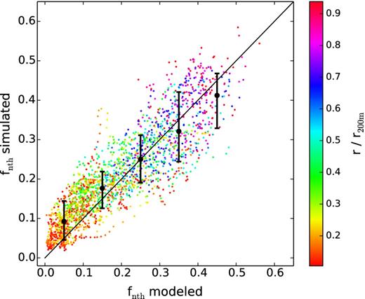
Comparison of the modelled and simulated non-thermal fraction, fnth, of the mass-limited sample. Each point on the scatter plot shows one radial bin of one cluster in the sample, and is colour-coded according to the central radius of the bin relative to r200 m. Only radial bins between 0.1 and 1 r200 m are shown. The black points with error bars show the median and 16/84 percentile of the distribution of fnth measured from the simulation in bins of modelled fnth values. The diagonal line shows the one-to-one correspondence.
Looking closer, the slight deviation of the black points from the one-to-one relation (the diagonal line) at large fnth values can be explained by the selection effect that only data points between 0.1 and 1r200 m are shown. The same selection effect does not seem sufficient to explain the deviation at small fnth values, and this may suggest a systematic tendency of a smaller modelled than simulated non-thermal fraction at r < 0.25r200 m. Although the statistical significance is only 1σ, we offer a possible explanation of this deviation in Section 5.
4.2 Effect of varying model parameters
The two parameters in the analytical model, η and β, are physical parameters related to turbulence injection and dissipation, respectively. However, their values are not yet well constrained from theory. In SK14, we find that ηβ ≈ 0.7 and β ≈ 1 provide excellent agreement between the model predictions and the fitting formulae derived from the existing observations (Arnaud et al. 2010; Planck Collaboration V 2013) and numerical simulations (Shaw et al. 2010; Battaglia et al. 2012). The same values reproduce the simulation outputs used in this paper.
To examine how sensitive the comparison results are to the exact values of η and β, we show the effects of varying them in Fig. 7. Each panel in Fig. 7 uses different values of β and η as shown, and the central panel with η = 0.7 and β = 1 is identical to Fig. 6.
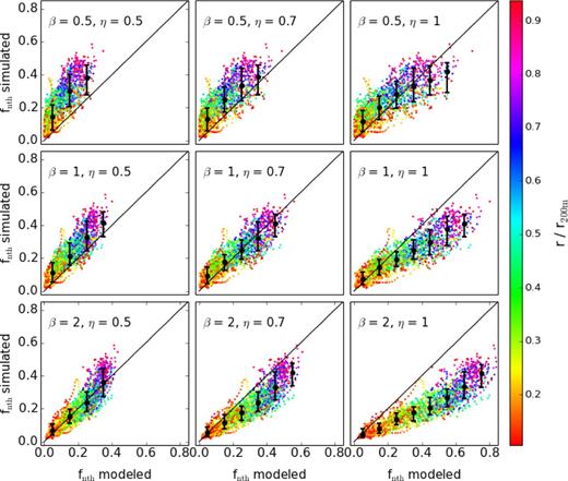
When the cluster mass growth is fast, i.e. when |$\sigma ^2_{\rm tot}$| increases with a time-scale tgrowth shorter than the turbulence dissipation time-scale td, the non-thermal fraction approaches η (section 3.2 in SK14). In the opposite case, the non-thermal fraction approaches ηtd/tgrowth ∝ ηβ. At z ≈ 0, td ≪ tgrowth in the inner region of a galaxy cluster, whereas td/β is comparable to tgrowth in the outskirts. This suggests that fnth is roughly proportional to ηβ when β < 1, and the shape of the radial dependence of fnth is mainly given by the increase of the dynamical time with radius. For larger values of β, the radial dependence of fnth should flatten towards large radii due to the saturation of fnth to the value of η in the fast growth regime.
These features are clearly visible in Fig. 7: the slope of the modelled versus simulated fnth relation is primarily determined by ηβ, and the curvature of the relation by β. As far as the slope is concerned, the three panels on the diagonal from bottom left to top right with 0.5 ≤ ηβ ≤ 1 provide a good match between the modelled and simulated values. From the curvature of the relation, the central panel with the default parameter values give the best agreement, in the sense that the scatter of the data points at each radius (with each colour) is most symmetric around the one-to-one relation.
4.3 Dynamical state
SK14 used the analytical mean mass accretion history of Zhao et al. (2009) to show that the average non-thermal pressure fraction increases with the cluster mass and redshift. This feature is hard to test directly with the simulated cluster sample described in Section 2 due to the limited range of masses and redshifts for which the profiles of the clusters are well resolved. Also, as discovered by NLN14, the redshift and mass dependences are greatly reduced when the cluster radius is scaled by r200 m.
Still, we can divide the simulated cluster sample by their accretion histories, and test whether the model and the simulation yield the same difference on fnth between the sub-samples. Since the model attributes the origin of the mass and redshift dependences of fnth to the dependence on the recent mass accretion history, this provides a more direct test of the model prediction than comparing the average non-thermal pressure fraction of cluster samples at different redshift or with different masses.
The distribution of Γ200 m in the mass-limited cluster sample is shown in Fig. 8. We select two sub-samples of the simulated clusters with Γ200 m < 1.8 and Γ200 m > 2.7, respectively. Both sub-samples contain 23 galaxy clusters. We apply the analytical model to each cluster in the sub-sample and compare the mean fnth profile of each sub-sample with the corresponding simulated one. As shown in Fig. 9, the sub-sample with higher recent mass growth has a significantly higher non-thermal pressure fraction at all radii. This is consistent with the previous numerical studies (e.g. Nagai et al. 2007; Piffaretti & Valdarnini 2008; Nelson et al. 2012) which consistently find a larger hydrostatic mass bias for less relaxed, recently merged clusters. This difference in the average non-thermal pressure fraction is remarkably well reproduced by the analytical model. This result reinforces the basic underlying physical picture that intracluster turbulence is triggered during the cluster mass assembly, and that the kinetic energy in the intracluster turbulence is derived ultimately from the gravitational energy released during the structure growth.
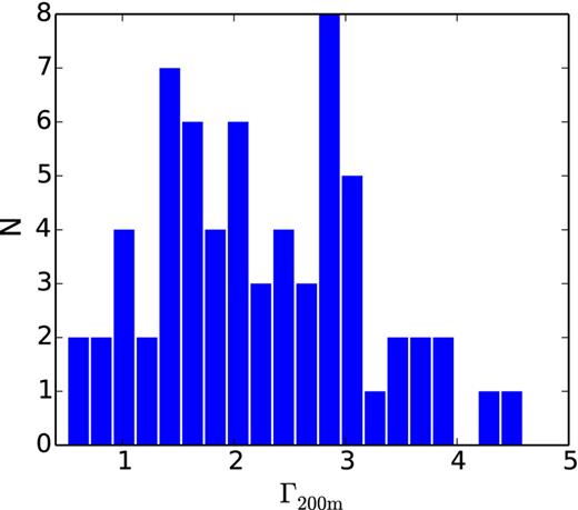
Distribution of the proxy of the accretion history and dynamical state, Γ200 m, computed from the mass-limited sample of simulated galaxy clusters.
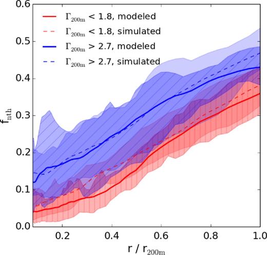
Modelled and simulated fnth profiles of an early growth sub-sample (Γ200 m < 1.8, blue lines) and a late growth sub-sample (Γ200 m > 2.7, red lines). The lines and the shaded regions are the mean profile of the sample and the 16/84 percentiles, respectively.
In Fig. 10, we compare the modelled and simulated non-thermal fractions in each radial bin of each cluster in the two sub-samples. It is clear that, for the early accretion (Γ200 m < 1.8) sub-sample which consists of more dynamically relaxed clusters at the time of comparison (z = 0), the scatter between the modelled and simulated fnth values is smaller. This is in accord with the expectation that the analytical model works better for dynamically relaxed clusters. Nevertheless, a clear correlation exists also for the more disturbed clusters (Γ200 m > 2.7), suggesting that the analytical model is also applicable to these systems in estimating the turbulence pressure, though with greater noise.
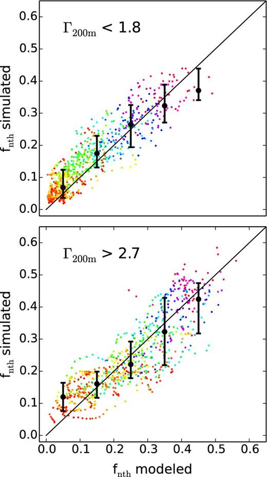
Comparison of modelled and simulated fnth of the early growth sub-sample (upper panel) and the late growth sub-sample (lower panel). In each panel the symbols are the same as those in Fig. 6.
We note that the Γ200 m parameter used in this paper is not optimal as a proxy for the dynamical state, since it is defined with the mass increase between two snapshots. By definition, the dynamical state of a cluster can be determined by its temporary state. A dynamical state proxy defined at a single snapshot based on the dynamical properties of the halo particles would be more convenient to use, and at the same time provide a more direct characterization of the deviation from hydrostatic equilibrium. For future studies of assigning the non-thermal pressure profile to dark matter haloes extracted from the dark-matter-only N-body simulation, such more advanced dynamical state proxy may be preferred.
5 DISCUSSION: TEST OF THE PHYSICAL PARADIGM
Evolution of the intracluster turbulence is a problem involving a vast range of spatial and time-scales. The relevant physical processes include the cluster mass assembly in a cosmological context, the merger and accretion shocks which convert the bulk kinetic energy into the turbulence kinetic energy and heat, and the detailed intracluster gas dynamics associated with the development and cascade of turbulence. Simulating all of them with sufficient numerical precision is beyond the reach of a single set of numerical simulations. Simulations dedicated to certain physical processes would be needed for testing them in greater detail.
In this respect, the large-size cosmological simulation used in this paper is ideal for testing the relation of turbulence growth with cluster mass assembly in a cosmological context, for which the picture underlying the analytical model has been verified by the positive results presented in Section 4. On the other hand, cosmological simulations of a single cluster (e.g. Vazza et al. 2009, 2011; Paul et al. 2011; Miniati 2014) are better suited for studying mechanisms of turbulence injection, and high-resolution simulations performed on a fixed grid (Gaspari & Churazov 2013; Gaspari et al. 2014) are better suited for studying the turbulence cascade process. The insights gained from these dedicated simulations can be easily incorporated into the analytical model.
For a precise assessment of the amplitude of intracluster turbulence pressure, it is important to know the effective thermalization ratio at turbulence injection, and the turbulence dissipation time-scale. In the framework of the SK14 analytical model, this suggests the need to determine the values of the model parameters η and β and investigate their possible dependence on radius, redshift, and cluster mass. These can in principle be realized by dedicated numerical simulations, when numerical effects in these simulations are well understood and controlled. Recently, using the moving-mesh numerical scheme, Schaal & Springel (2015) reported a higher energy dissipation fraction contributed by shocks in the warm hot intergalactic medium, and correspondingly a higher average Mach number of shocks at which the bulk of energy dissipates, than previous studies performed with the Adaptive Mesh Refinement technique (e.g. Ryu et al. 2003; Pfrommer et al. 2006; Kang et al. 2007; Vazza et al. 2011; Planelles & Quilis 2013). This, if confirmed, would suggest a higher thermalization ratio, and that a radius and redshift dependence of η would be determined by the relative importance of the high Mach number accretion shocks and the low Mach number internal shocks.
We note that the SK14 analytical model is not consistent with the long-term power-law decay behaviour expected for the turbulence kinetic energy (Landau & Lifshitz 1959; Frisch 1995; Subramanian, Shukurov & Haugen 2006). This inconsistency is due to our assumption of a one-to-one relation between the cluster radius and the turbulence dissipation time-scale, which is the ratio of the size and velocity of the largest eddies, at that radius (i.e. td ∝ tdyn). The consequence of this assumption is most visible in the regions where turbulence dissipates much faster than it grows, and may have contributed to the possible systematical difference between the modelled and simulated fnth at small radii. To correct for this, one may need to include a spectral dimension to the model, that is to keep track of the power spectrum of turbulence velocity field at each radius as a function of time. This, in turn, will allow for an easier link to intracluster magnetic fields and cosmic rays.
6 CONCLUSION AND PERSPECTIVES
We have compared the SK14 analytical model for the turbulence pressure inside galaxy clusters to a state-of-the-art hydrodynamics numerical simulation. The analytical model and the simulation outputs show excellent agreement on the non-thermal pressure fraction on a cluster-by-cluster basis − both its radial profile and its dependence on the cluster mass accretion history.
This demonstrates that the SK14 model in its current form can already be used to predict the amplitude of intracluster turbulence pressure with a precision comparable to that of the state-of-art cosmological hydrodynamics simulations. This opens up an exciting possibility that we may be able to use the analytical model to correct the systematic bias in the mass estimation of galaxy clusters due to the turbulence pressure. The analytical model, in turn, would also provide a convenient and efficient way to interpret the SZ power spectrum and observations of cluster outskirts from ongoing and upcoming large cluster surveys.
At the same time, the comparison results show that a simple analytical model can indeed capture the basic physical processes related to the evolution of intracluster turbulence pressure. In particular, our comparison study has verified the underlying physical picture that the turbulence growth is determined by cluster mass assembly in a cosmological context. The detailed physics regarding injection and dissipation of intracluster turbulence requires further tests from comparisons with dedicated high-resolution simulations of individual clusters. We point out that adding a spectral dimension to the model may lead to a better description of the long-term dissipation of the turbulence, further improve the consistency with simulations in the inner regions of clusters, and provide a framework for a unified understanding of non-thermal phenomena in galaxy clusters.
XS thanks Massimo Gaspari for helpful discussions. KL and DN acknowledge support from NSF grant AST-1009811, NASA ATP grant NNX11AE07G, NASA Chandra grants GO213004B and TM4-15007X, and the Research Corporation. This work was supported in part by the facilities and staff of the Yale University Faculty of Arts and Sciences High Performance Computing Center. We thank Erwin Lau and Peng Oh for comments on the draft.
Alternatively, one may compute |$\sigma ^2_{\rm tot}$| from Ptot which by itself is computed using the hydrostatic equilibrium equation, and then derive |$\sigma ^2_{\rm nth}$| as the difference of |$\sigma ^2_{\rm tot}$| and Pth/ρgas. Since simulated galaxy clusters are not spherically symmetric nor fully relaxed, this alternative method yields slightly different |$\sigma ^2_{\rm tot}$|. While the |$\sigma ^2_{\rm tot}$| profiles of the cluster sample computed with the two methods are very similar in the virial region of the clusters, the |$\sigma ^2_{\rm nth}$| profiles are significantly different because the alternative method computes |$\sigma ^2_{\rm nth}$| as the difference of two large quantities. Since |$\sigma ^2_{\rm nth}$| computed this way is more prone to numerical errors, we choose the method described in the main text to compute |$\sigma ^2_{\rm nth}$| and |$\sigma ^2_{\rm tot}$|.
REFERENCES
APPENDIX A: MEASURE GAS VELOCITY DISPERSION FROM SIMULATION
Following NLN14, we measure the non-thermal velocity dispersion of the gas σnth in radial shells after subtracting the mean velocity of the shell with respect to the centre-of-mass velocity of the total mass interior to this radial shell. In order to remove the kinetic energy associated with sub-structures which does not contribute to the pressure of the global intracluster gas, we also exclude the contribution from gas that lies in the high-density tail in the probability distribution of gas densities according to the procedure presented in Zhuravleva et al. (2013). We show the effect of removing the sub-structures to the σtot and σnth profiles in Fig. A1. The sub-structures generally affect σnth more than σtot. Without removing them, the non-thermal fraction measured from simulations would be slightly overestimated. No strong trend of sub-structure influence with accretion history is observed. In addition to sub-structure removing, we smooth the profiles with the Savitzky–Golay filter used in Lau et al. (2009).
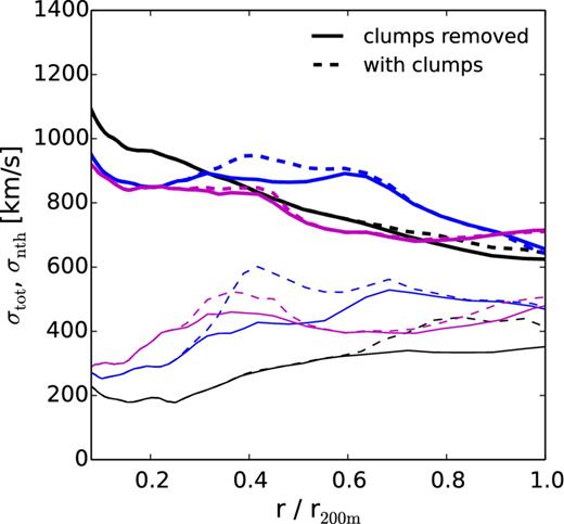
Measured σtot (thick lines) and σnth (thin lines) profiles with and without removing the sub-structures (clumps) in the simulation. Profiles for three clusters at z = 0 with various mass accretion histories are presented (black: early accretion; blue: medium; magenta: late accretion). All three chosen clusters have masses close to the median mass of the sample.
We note that there are different choices of the mean velocity to be subtracted from the velocity field when computing non-thermal velocity dispersion from simulations. They correspond to different ways of decomposing the velocity field. Studies focusing on the turbulence properties in the inertial range usually adopt the averaged velocity in a local volume as the mean velocity (see e.g. Vazza, Roediger & Brüggen 2012). This decomposes the velocity field into parts that are smaller or larger compared to the size of the chosen local volume, which are usually referred to as ‘turbulence’ and ‘bulk motion’, respectively. The spherical averaging method we use decomposes the velocity field into the average infall/outflow motion and the residual motions. These residual motions, which receive contribution from both turbulent random motion and some large-scale bulk motions, are the main source of the HSE mass bias. Further studies are required to gain more understanding of the nature of gas motions in the cluster outskirts. This would help distinguish the physical sources of the non-thermal velocity dispersions, and point to an optimal way of decomposing the velocity field that is conceptually clear and at the same time matches the methods used in analysing observations. For the moment, we stick to the spherical averaging method. The σnth measured this way is clearly defined, and its contribution to the hydrostatic mass bias is relatively well understood (Lau et al. 2013).
The velocity dispersions we measure here are averaged over all directions, but physically only the radial velocity dispersion contributes to the pressure support against gravity. Shown in Lau et al. (2009), Nelson et al. (2012) and NLN14, the gas motions are predominantly radial at cluster outskirts, especially near r200 m. The physical origin of the measured velocity anisotropy is not yet clear. Therefore, velocity anisotropy is so far dismissed in the analytical model and the comparison to simulations. Once the amplitude of velocity anisotropy and its radial dependence are known, it can be easily taken into account.
APPENDIX B: VISUALIZING PROPAGATION OF MERGER SHOCK
While inspecting the evolution of σtot in the simulations at fixed Eulerian radii, we discover some ‘wiggles’ – sharp rise and fall in σtot with time (Fig. 3). In Fig. B1, we show that there are indeed entropy jumps at the positions of these ‘wiggles’, supporting that they originate from merger shocks. The magnitude of the jumps is typically ≲ 2, corresponding to low Mach numbers that are expected for the merger shocks. Note that the entropy in one shell also falls after the shock, likely due to the expansion of the shock-heated gas into a neighbouring shell at a larger radius.
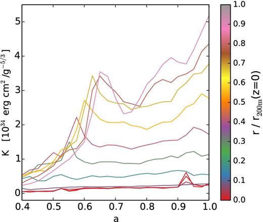
Evolution of the average entropy |$K \equiv T/\rho _{\rm gas}^{2/3}$| in Eulerian shells for the same simulated cluster used for Fig. 3, where the mass-weighted temperature T and the gas density ρgas are averaged in the shell.
These low Mach number merger shocks are close to sound waves – they are more efficient in compressing the gas than increasing its entropy. Adiabatic compression contributes to most of the temperature jump at these shocks. As a consequence, the temperature experiences an evident jump at the shock, and falls close to its original value after the shock passes. The temperature map, therefore, enables one to see the propagation of the shock. In Fig. B2, one sees spatially coherent high-temperature regions elongated in the azimuthal direction, indicative of shock fronts. The expansion of the shock fronts inside the cluster coincide with the increase of peak radius of the corresponding ‘wiggles’ in Figs 3 and B1 (white dashed circles).
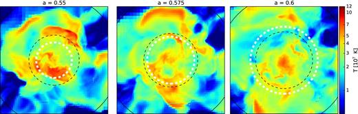
Gas temperature distribution of the simulated cluster used for Figs 3 and B1 at three consecutive snapshots. The size of the images is 4 Mpc h−1, and the mass-weighted temperature is averaged in a slice of thickness ≃ 500 kpc h−1 across the cluster centre. The white dashed circles mark the radial location of the peak in the σtot profile that corresponds to the ‘wiggles’ in Fig. 3 between a = 0.5 and 0.7. Note that the radial extension of the ‘wiggles’ is large, as can be seen from Fig. 3. The black dashed and solid circles show the position of r200 m at the time of the snapshot and at z = 0, respectively.
In one dimension, due to the projection effect and the possible intrinsic asymmetry of shock fronts in different azimuthal directions, shocks are much more prominent as ‘wiggles’ in temperature or σtot against time rather than against radius. Thus, plots like Figs 3 and B1 can better depict the propagation of shocks than profiles of thermodynamical quantities.
