


Abstract
This paper explores if the mean properties of early-type galaxies (ETGs) can be reconstructed from ‘genetic’ information stored in their globular clusters (GCs; i.e. in their chemical abundances, spatial distributions and ages). This approach implies that the formation of each globular occurs in very massive stellar environments, as suggested by some models that aim at explaining the presence of multipopulations in these systems. The assumption that the relative number of GCs to diffuse stellar mass depends exponentially on chemical abundance, [Z/H], and the presence of two dominant GC subpopulations (blue and red), allows the mapping of low-metallicity haloes and of higher metallicity (and more heterogeneous) bulges. In particular, the masses of the low-metallicity haloes seem to scale up with dark matter mass through a constant. We also find a dependence of the GC formation efficiency with the mean projected stellar mass density of the galaxies within their effective radii. The analysis is based on a selected subsample of galaxies observed within the ACS Virgo Cluster Survey of the Hubble Space Telescope. These systems were grouped, according to their absolute magnitudes, in order to define composite fiducial galaxies and look for a quantitative connection with their (also composite) GCs systems. The results strengthen the idea that GCs are good quantitative tracers of both baryonic and dark matter in ETGs.
1 INTRODUCTION
The characteristics of living creatures, as well known, can be linked to their DNA properties. In a similar fashion we may ask if, given the features of a globular cluster system (GCS; defined in terms of spatial distribution, chemical composition and ages), they can yield ‘genetic’ information about the field stellar populations of the early-type galaxies (ETGs) they belong to. This question can be extended to late-type galaxies regarding the formation of their stellar haloes and bulges.
A number of papers in the literature have pointed out differences between field stars and globular clusters (GCs) rather than similarities (e.g. Kissler-Patig 2009). Although such differences should take into account that GCS properties come in number weighted form, contrasting with those of galaxy properties, that we read in a luminosity weighted way, the generalized conclusion seems to indicate that GCs and field stars have followed different formation histories.
In the meantime, the discovery of multistellar populations in GCs suggests processes where the GC formation was ‘a for more titanic event than ever imagined before’ (see Renzini 2013). These scenarios involve large amounts of field stars per GC that would share some characteristics of the clusters (D'Ercole et al. 2008; Carretta el al. 2010).
Despite some difficulties (e.g. the required high star formation efficiencies; see Bastian et al. 2013), these models seem consistent with the idea that GCs could be tracers of much more massive diffuse stellar populations. This kind of approach was explored in Forte, Faifer & Geisler (2005, hereafter FFG05), Forte, Faifer & Geisler (2007, hereafter FFG07), Forte, Vega & Faifer (2009, hereafter FVF09) and Forte, Vega & Faifer (2012, hereafter FVF12).
In a recent paper, Harris, Harris & Alessi (2013, hereafter HHA13) present an extensive compilation of several structural parameters that characterize GCS and their parent galaxies. These authors also discuss the implications of a number of correlations that arise considering GCs as a whole, i.e. not including the effects of GCs subpopulations. One of their conclusions indicates that the total number of GCs is not a good estimator of the total stellar mass of a galaxy. In fact, a linear log–log fit between these quantities shows deviations both at the low and high galaxy mass regimes.
They also show that, in a GC population so defined, there is a clear trend between the mass fraction locked in GCs, Sm, and the total stellar galaxy mass that adopts a U-shaped form, already noted by Peng et al. (2008), in terms of the GC specific frequencySn (number of GCs per V-luminosity in MV = −15 units). HHA13 interpret that this shape is the consequence of a decrease of the star formation efficiency, both at the low and high mass regimes produced by mass loss and by the energetic events connected with the nuclei of galaxies, respectively.
In this paper we attempt to elaborate further on those results by introducing the effect of GC bi-modality, i.e. the presence of blue and red GCs. In particular, we aim at exploring the usefulness of these distinct GC populations to trace large-scale features of galaxies as, total stellar mass, the relative contribution of haloes and bulges to that mass, chemical abundances, stellar mass to luminosity ratios and, indirectly, dark matter (DM) content.
A preliminary attempt to link galaxies with their GCS in terms of the blue and red populations was presented in FVF09 for galaxies observed within the ACS Virgo Cluster Survey of the Hubble Space Telescope (Côté et al. 2004). In this work, we revise that approach taking advantage of later developments, namely, the accessibility to the original photometry of GCs in the ACS Virgo galaxies (Jordán et al. 2009), the multicolour photometry of these galaxies (Chen et al. 2010) and the C-griz’ colour–metallicity grid from Forte et al. (2013, hereafter F13).
As in previous works, we stand on the idea that GC formation is not a singular event but, rather, is associated with large volumes of star formation that eventually lead to the origin of distinct populations: a low metallicity and spatially extended stellar halo, associated with the blue globulars, and a more concentrated and chemically more heterogeneous stellar population, connected with the red GCs. The presence of extended low-metallicity haloes has been noticed by different means, for example, in NGC 3379 (Harris et al. 2007) and NGC 4472 (Mihos et al. 2013).
This work assumes that the GCs colour bi-modality is the consequence of the genuine bimodal nature of their chemical composition distributions (see Brodie et al. 2012), i.e. not an artefact of some eventually non-linear integrated colour–metallicity relations. On the other side, and as noted in F13, this last kind of relations does not reject necessarily the possibility of a genuine chemical bi-modality.
The paper is organized as follows. The definition of fiducial galaxies is given in Section 2. The analysis of the GCs colour distributions, as well as their modelling in terms of chemical abundance, is described in Section 3. The link between GCs and the diffuse stellar populations of the galaxies is presented in Section 4, while the photometric scales for GCs and galaxies are discussed in Section 5. The model results based on galaxy colours and integrated brightness are discussed in Section 6. The analysis of the shape of the relation between total number of GCs and galaxy masses is presented in Section 7. The connection between the Sérsic parameter and the projected stellar surface mass density for the fiducial galaxies is presented in Section 8. The results of modelling the low-metallicity stellar halo, bulge-like component and total stellar masses, as well as the GC formation efficiency, are presented in Section 9. The relation between the DM content of each galaxy and their low-metallicity stellar haloes is discussed in Section 10. The case of the Fornax spheroidal galaxy is described in Section 11, and the final conclusions are given in Section 12.
2 THE DEFINITION OF FIDUCIAL GALAXIES AND THEIR GCs
One of the problems in looking for a GC-field stars connection is the noise inherent to the counting statistics of GCs, an effect that becomes more severe as the galaxy is fainter and the number of associated GCs is lower. In order to decrease this effect we ‘merge’ both the stellar and GCs populations of Virgo ACS galaxies creating fiducial galaxies. For this purpose, we compose the g and z brightness (through the observed flux in each band) in order to derive the integrated magnitudes and (g − z) colours of each fiducial galaxy.
This approach would work only if there is a pattern, common to all galaxies, linking the features of field stars and their GCS. The idea also assumes that the bulk of field stars and GCs are mostly coeval or spread over a limited range of ages. This seems to be true, at least for galaxies of the ‘red sequence’ (or see Norris et al. 2008, for the particular case of NGC 3923).
The fiducial systems contain a given number of galaxies, ordered by decreasing brightness in the g band, and were defined trying to fulfil two conditions. On one side, they should have a sufficiently large number of GCs to allow a proper fit of their composite colour histograms and, on the other, a significant separation in terms of the mean absolute magnitudes of consecutive fiducial galaxies (at least ≈0.5 mag).
In this work we adopt the ugriz′ galaxy photometry extensively discussed by Chen et al. (2010) although we restrict our analysis only to the (g − z) colour index. In the case of the GCs we use the photometric g and (g − z) data presented by Jordán et al. (2009), after taking into account completeness and field contamination (see below).
From the whole Virgo ACS galaxy sample (100 galaxies), we remove galaxies without distance moduli in Mei et al. (2007) as well as particular subgroups as the ‘blue cloud’ or ‘red compact’ dwarfs (Smith Castelli et al. 2013). We also rejected galaxies in frames contaminated by the GCs of massive neighbours and those that, after removing field contamination, lead to a null content of GCs. This procedure leaves a total sample of 67 galaxies.
An estimate of field contamination was carried out by selecting 12 galaxies with less than 10 globulars and considering as possible field interlopers all those objects with galactocentric distances larger than 30 arcsec. This statistic, scaled by field size and number of galaxies composing a given fiducial galaxy, was subtracted from the composite GC (g − z) colour histograms.
Regarding the limiting magnitude that assures an acceptable degree of completeness, we compared the number of GCs bluer and redder than (g − z) = 1.2, in 0.5 mag intervals in the g band. The ratio between these numbers for the whole GC sample in Jordán et al. (2009) shows a detectable deficit of blue globulars for objects fainter than g = 25 mag, a brightness that we adopt as the limit of our statistic. Under the assumption that GCs have fully Gaussian-integrated luminosity functions, with a mean value g ≈ 23.85, that limit leaves out some 15 per cent of the total cluster population.
Finally, we are left with a total of 5470 GCs in 67 galaxies that define nine fiducial galaxies. The first fiducials, due to their brightness and well populated GCS, contain five, three and five galaxies, respectively. In particular, the two first composite galaxies appear above the magnitude gap at MV ≈ −20.5 detectable in the colour–magnitude diagram (see e.g. Smith Castelli et al. 2013).
In what follows, the interstellar reddening corrections were derived by adopting E(g − z) = 2.15 E(B − V) and the colour excesses listed by Ferrarese et al. (2006) which, in turn, are based on the Schlegel, Finkbeiner & Davis (1998) maps.
The absolute magnitude Mg versus intrinsic colour (g − z)0 relation for the galaxy sample, corresponding to a mean colour excess E(g − z) = 0.065 and mean interstellar extinction Ag = 0.050, is shown in Fig. 1, where the straight line has the same slope of the fit presented by Smith Castelli et al. (2013) in their study of the colour–magnitude relation of the ACS Virgo cluster galaxies. The galaxy members (identified by their VCC numbers) that define a given fiducial galaxy, as well as their composite absolute Mg magnitudes, (g − z) colours and average effective radii (computed from the data given by table 2 in Chen et al. 2010) are presented in Table 1.
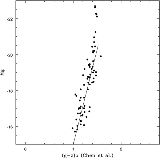
Absolute magnitude Mg versus (g − z)0 colour for the selected Virgo ACS sample including 67 galaxies. The straight line has the slope of the relation found by Smith Castelli et al. (2013; see text).
Parameters of the fiducial galaxies.
| Fiducial | Ngal | Mg | (g − z)0 | |$(g-z)_{\rm mod}^a$| | MV | reff (kpc) |
|---|---|---|---|---|---|---|
| 1 | 5 | −22.40 | 1.48 | 1.45 | −22.86 | 13.1 |
| 2 | 3 | −20.99 | 1.46 | 1.41 | −21.44 | 4.7 |
| 3 | 5 | −20.28 | 1.45 | 1.39 | −20.73 | 2.5 |
| 4 | 9 | −19.51 | 1.41 | 1.39 | −19.95 | 1.4 |
| 5 | 10 | −18.92 | 1.37 | 1.37 | −19.35 | 1.2 |
| 6 | 10 | −18.35 | 1.31 | 1.29 | −18.77 | 1.7 |
| 7 | 10 | −17.30 | 1.16 | 1.22 | −17.68 | 1.7 |
| 8 | 9 | −16.70 | 1.19 | 1.14 | −17.09 | 0.9 |
| 9 | 8 | −16.10 | 1.13 | 1.12 | −16.47 | 1.1 |
Note. Galaxies in each of the nine fiducial galaxies identified by their VCC number: 1 – 1226, 881, 763, 1316, 1978; 2 – 1632, 1903, 1231; 3 – 1154, 2092, 759, 1062, 1030; 4 – 1692, 1938, 1664, 944, 1720, 654, 1279, 2000, 778; 5 – 1883, 1242, 355, 784, 1619, 1250, 369, 1146, 1303, 828; 6 – 1630, 698, 1537, 1913, 1321, 1283, 1475, 1178, 1261; 7 – 9, 1087, 1422, 437, 1861, 140, 1910, 856, 543, 1355; 8 – 2019, 1431, 1528, 1833, 200, 1440, 751, 1545, 1049; 9 – 1075, 1828, 1407, 1512, 1185, 2050, 1826, 230.
a(g − z) colours in the scale of Chen et al. (2010); (g − z) model colours +0.13 mag.
In the case of the brightest galaxies, the areal coverage of the Virgo ACS is not large enough for a complete analysis of their GCS. This is illustrated in Fig. 2 where the short vertical line indicates the size (in kpc) corresponding to 100 arcsec at the mean distance of the Virgo cluster (see also Smith Castelli et al. 2013).
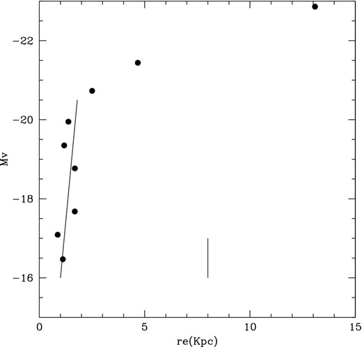
Absolute magnitude MV versus effective radii for nine fiducial galaxies resulting from composing the Virgo ACS galaxies shown in Fig. 1. The short vertical line indicates a radius of 8 kpc, 100 arcsec at the distance of the Virgo cluster (adopting a mean distance moduli (m − M)0 = 31.1).
In order to estimate the total number of GCs in each fiducial galaxy we used the data given in HHA13 (their table 4). First, we grouped the galaxies defining each fiducial and then made a regression of the number of GCs in the ACS galaxy sample versus those coming from that paper. This analysis indicates that significant corrections to the number of GCs are only required for the three brightest fiducial galaxies.
A further step for these galaxies is a tentative estimate of the distribution of their GCs in terms of the blue and red subpopulations, a matter complicated by the different spatial scale lengths of these populations. That is, red GCs are usually more concentrated towards the galaxy centres than their blue counterparts, leading to a change of the GCs number ratio along the galactocentric radius.
In these cases, and for illustrative purposes, we take the giant ellipticals NGC 1399 and NGC 4486, for which wide field studies are available (see e.g. FFG07). In the first galaxy the GC subpopulation splits by ≈50 per cent, while for NGC 4486 the blue and red GC populations follow a proportion of 70 per cent of blue and 30 per cent of red GCs. As a compromise, we adopt indicative values of 65 and 35 per cent, respectively.
The corrections inferred for the blue and red populations of the three brightest fiducials galaxies are given in Table 2. We warn the reader about the uncertainties involved (and also recall the inherent comments in HHA13). The last two columns in this table give the mean number of blue and red GCs after correcting for areal completeness.
Fit parameters for the GC colour histograms.
| Fiducial | Nb | Zsb | Nr | Zsr | Δlog (Nb) | Δlog (Nr) | χ2 | log 〈Nb〉c | log 〈Nr〉c |
|---|---|---|---|---|---|---|---|---|---|
| 1 | 1100 | 0.05 | 1852 | 1.10 | 1.17 | 0.54 | 0.98 | 3.515 | 3.304 |
| 2 | 260 | 0.05 | 511 | 0.70 | 0.76 | 0.37 | 0.62 | 2.530 | 2.486 |
| 3 | 240 | 0.035 | 383 | 0.55 | 0.24 | 0.10 | 1.26 | 1.919 | 1.982 |
| 4 | 400 | 0.030 | 373 | 0.55 | – | – | 1.01 | 1.643 | 1.613 |
| 5 | 260 | 0.030 | 353 | 0.45 | – | – | 0.44 | 1.415 | 1.544 |
| 6 | 270 | 0.035 | 175 | 0.35 | – | – | 1.09 | 1.431 | 1.230 |
| 7 | 180 | 0.020 | 92 | 0.25 | – | – | 0.48 | 1.255 | 0.954 |
| 8 | 160 | 0.020 | 50 | 0.15 | – | – | 0.63 | 1.255 | 0.778 |
| 9 | 100 | 0.020 | 24 | 0.15 | – | – | 0.59 | 1.096 | 0.477 |
| 9b | 124 | 0.020 | 0 | – | – | – | 1.00 | 1.193 | – |
Note. 〈Nb〉c: mean corrected number of blue GCs; 〈Nr〉c: mean corrected number of red GCs; 9b: best-fitting solution assuming a single blue GC population.
3 GLOBULAR CLUSTER COLOUR DISTRIBUTIONS
The basic ideas for modelling the GC colour histograms were previously explained in FFG07, FVF09 and FVF12, and assume the existence of two distinct GC subpopulations: the so-called blue and red GCs. Note that this is a matter of working nomenclature as the red GCs are in fact redder (but not much in some of the low-mass galaxies) than those that define the omnipresent blue GC subpopulation.
As explained in those papers, we use a Monte Carlo generator to create seed GCs with a distribution in chemical composition Z controlled by a scale length Zs (measured in Z⊙ units in what follows and listed in Table 2), and defined between a lowest value Zi and an upper limit Zsup. For both subpopulations we adopt Zi = 0.014 Z⊙ (the lowest value in the colour–metallicity calibration), while for Zsup we adopt 1.0 and 2.3 Z⊙ for the blue and red GCs, respectively. The lowest chemical abundance corresponds to [Fe/H] ≈ −2.2 adopting an α ratio in the range of 0.3–0.4.
In our approximation, both GC subpopulations, as mentioned before, exhibit some degree of overlapping in metallicity (depending on the Zs parameters). This has similarities with the situation reported by Leaman, VandenBerg & Mendel (2013) for Milky Way clusters. These authors find a ‘bifurcated’ age–metallicity relation, i.e. the presence of two sequences sharing the same age spread (≈2 Gyr), shifted in mean metallicity, and exhibiting a range where both (halo and disc) GC populations share the same metallicity. As discussed in F13, such an age spread would be undetectable by photometric means.
The GC colour histogram fits were performed in a similar way for the blue and red clusters except that, for the first subpopulation, we added an empirical value ΔZ = 0.65(g − 22.35) to their Zsb in an attempt to mimic the mass–metallicity relation observed for these clusters (see e.g. Mieske 2006, 2010; Harris 2009). This parameter is set to zero for GCs fainter than g = 22.35.
The parameters that deliver the best fits to the (composite) observed (g − z)0 histograms are listed in Table 2. The number of GCs and the Zs scales of each subpopulation were iterated aiming at minimizing the (inverse) quality fit indicator χ2 defined by Côté, Marzke & West (1998). Typical errors, estimated as in F13, are ±0.01 in Zsb, ±0.05 in Zsr and ±0.1 in the ratio of blue to red GCs.
We note that the less massive fiducial (number 9) still has a detectable number of ‘red’ GCs that we identify as a bulge-like component. For illustrative purposes, we also give the best fit corresponding to a single GC population of blue GCs. Both data points will be shown linked by a line in a number of diagrams that follow.
The GC colour histograms are depicted in Fig. 3, where the panels are presented from left to right and down (in order of decreasing galaxy brightness) and show a feature already noticed by Peng et al. (2006), i.e. that bi-modality becomes less evident with decreasing galaxy brightness and disappears for the faintest galaxies. While the blue GC component is present in all the galaxies, the red GCs increase their relative importance in number, as well as their chemical scale length, as the galaxy mass increases. In what follows, we identify the blue GCs with the diffuse low-metallicity stellar population, the ‘halo’ and the red GCs with the ‘bulge-like’ stellar population.
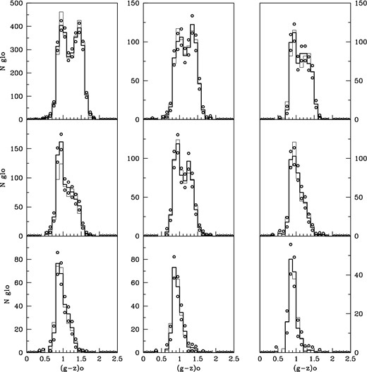
Observed and model (g − z) colour histograms for GCs in the nine composite galaxies (black and grey lines, respectively). The open dots represent the formal counting uncertainty in each (0.1 mag) colour bin. The absolute g brightness of each fiducial galaxy decreases to the right and down.
The composite observed GC colour–magnitude diagram, and the modelled ones, for all the fiducial galaxies are shown in Fig. 4. A comparison shows an acceptable similarity although some differences exist. On one side, the observed sample exhibits a number of objects bluer than (g − z)0 = 0.70, possibly a combination of field interlopers and larger photometric errors. The upper bright region of the observed red GCs domain is clearly more populated than the model. In this case, we speculate that these objects might be GC–ultra-compact dwarf transition objects (see e.g. Faifer et al. 2011).
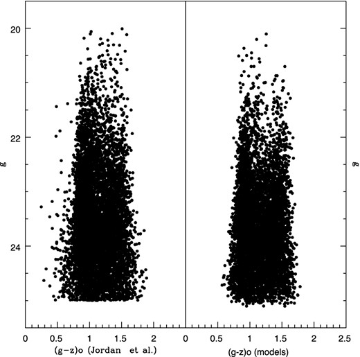
Left-hand panel: composite colour–magnitude diagram for 5467 GCs associated with the 67 galaxies discussed in the text, adopting a limiting magnitude g = 25.0 mag. Right-hand panel: composite diagram showing the model GCs that deliver the best fits to the (g − z)0 colour histograms of GCs in the fiducial galaxies. The origin of the differences seen in both panels is commented in the text.
4 THE GC-FIELD STARS CONNECTION
The basic idea behind equation (5) is that each GC is formed within a much more massive stellar ‘unit’. Each unit shares the colour of the GC and its (M/L) ratio is dependent on the chemical abundance [Z/H]. In particular, the parameter δ controls the mass of field stars per GC at a given [Z/H] and, after integrating over the whole metallicity range, determines the overall (M/L) ratio and integrated colours of a given galaxy. In turn, a proper value of the Γ parameter leads to its integrated absolute magnitude (Mg, in our case). This relation has been successful in providing a good approximation to the shape of the brightness profile and colour gradient of the giant elliptical NGC 4486 over a galactocentric radius of 1000 arcsec (FVF12).
In this approach, the integrated colours of the ETGs will be determined by the luminosity weighted mass–metallicity spectrum of the stellar units that represent field stars. Without obvious star-forming processes, these colours should be confined to the GCs colour domain (see below).
5 PHOTOMETRIC SCALES FOR GLOBULAR CLUSTERS AND GALAXIES
As previously shown in FVF09, a comparison between the GCs (g − z)ACS colours presented in Peng et al. (2006; in the form of GC colour histograms) and those of the galaxies, from Ferrarese et al. (2006), suggests a zero-point difference between both data sets that is independent of magnitude. The (g − z) galaxy colours in this last work, in turn, are very similar to the colours given in the multicolour photometry presented by Chen et al. (2010), that we adopted in this paper.
In this section we revise the connection between the photometric scales through two different pathways.
By analysing the galaxy–GCs colour difference in two galaxies for which we have independent photometric data sets: NGC 4649 and NGC 4486.
Using the results of our galaxy colour modelling for 10 of the brightest galaxies in the sample.
Goudfrooij & Kruijssen (2013) noted that there is a significant colour difference between the red GCs (defined as having (g − z)ACS > 1.2) and the galaxy colours, six of them included in our analysis. These authors suggest that the difference arises as a consequence of a ‘bottom heavy’ luminosity function for the field stars in these massive galaxies that would be different from that prevailing in GCs. We return to this subject later in this section.
5.1 The galaxy–GCs colours in NGC 4486 and NGC 4649
Aiming at decreasing the effects of incompleteness in the GC samples due to the bright inner regions of the galaxies, we restrict our analysis to the galactocentric range defined between 50 and 100 arcsec, and to clusters brighter than the turnovers of the integrated luminosity function at g ≈ 23.85 (Villegas et al. 2010).
In the case of NGC 4486 we use the (C − T1) GCs photometry presented in F13. There is no (C − T1) colour profile available for this galaxy and, then, we adopted the (B − V) surface photometry given by Zeilinger, Moller & Stiavelli (1993). This photometry, in very good agreement with the (B − V) colours obtained by extrapolating (inwards) the colour profile presented by Rudick et al. (2010), gives (B − V)0 = 0.93.
For 458 GCs in NGC 4486, we obtained a mean colour (C − T1)0 = 1.51. From these last relations, (B − V)0 = 0.81 and then galaxy–GC colour differences Δ(B − V) = 0.13 and Δ(C − T1) = 0.28. In turn, from the colour–colour relations in F13, we infer Δ(g − z) = 0.24.
Alternatively, the GCs photometry from Jordán et al. (2009) yields a mean (g − z)0 = 1.16 for 435 clusters brighter than the turnover at g = 23.85, while the galaxy photometry by Chen et al. (2010) gives (g − z)0 = 1.54 and then Δ(g − z) = 0.39. This last colour difference results 0.15 mag larger than our previous estimate.
Faifer et al. (2011) presented gri′ Gemini photometry for GCs in NGC 4649, and for the inner region of the galaxy. The mean |$(g-i)^{\prime }_0$| colour of the GCs results 0.94 ± 0.03, while the galaxy halo colour is |$(g-i)^{\prime }_0=1.08$| (see their fig. 10). These values lead to a colour difference between the galaxy and its GCs of |$\Delta (g-i)^{\prime }_0= 0.14$| mag, and to Δ(g − z) = 0.20 mag from the relations in F13.
In turn, the (g − z)ACS photometry by Jordán et al. (2009) for 207 GCs, yields a mean colour (g − z)0 = 1.20, while the photometry given by Chen et al. (2010) indicates (g − z)C = 1.52, then leading to Δ(g − z) = 0.32 mag. That is, 0.12 mag larger than our estimate.
In what follows, we adopt a colour zero-point difference between the (galaxy) photometry of Chen et al. (2010)/Ferrarese et al. (2006) and the (GCs) photometry by Jordán et al. (2009) of +0.13 mag.
We cannot asses the origin of such a difference but note that Janz & Lisker (2009) have also pointed out that the (g − z) galaxy colours by Ferrarese et al. (2006) are systematically redder by about 0.1 mag compared with their own photometry.
5.2 Colour modelling for 10 bright galaxies
We selected the 10 brightest galaxies in the Virgo ACS sample after excluding VCC 798, which presents a blue central region indicating recent star formation, and VCC 1535 and VCC 2095 which are discy edge on galaxies. For these 10 galaxies we attempted our colour modelling, first by fitting the GC (g − z)ACS colour histograms (based on the Jordán et al. 2009 photometry), and then looking for a single δ parameter that leads to the integrated galaxy colours. For this approach, and given the large effective radii of these galaxies (comparable or larger than the ACS field; see Smith Castelli et al. 2013) we adopted the colours within 1 reff as given by Chen et al. (2010).
The results corresponding to δ = 1.9, and adding 0.13 mag to our model colours, are listed in Table 3. The mean residual in the (g − z) colours is 0.015 ± 0.038 mag, i.e. the models match the observed colours with a dispersion comparable to the photometric errors for the galaxies.
Model parameters for 10 bright galaxies of the ACS Virgo Cluster Survey.
| NGC | VCC | Nb | Zsb | Nr | Zsr | χ2 | (g − z)0 | (O − C)(g − z) |
|---|---|---|---|---|---|---|---|---|
| 4472 | 1226 | 170 | 0.05 | 330 | 1.20 | 0.83 | 1.51 | −0.02 |
| 4486 | 1316 | 400 | 0.05 | 838 | 1.15 | 1.19 | 1.55 | +0.01 |
| 4649 | 1978 | 200 | 0.06 | 385 | 1.30 | 0.69 | 1.52 | −0.02 |
| 4406 | 881 | 115 | 0.03 | 144 | 0.40 | 0.88 | 1.42 | +0.07 |
| 4374 | 763 | 174 | 0.03 | 189 | 0.60 | 0.70 | 1.41 | +0.00 |
| 4365 | 731 | 170 | 0.03 | 414 | 0.55 | 0.98 | 1.50 | +0.07 |
| 4552 | 1632 | 100 | 0.05 | 229 | 0.80 | 0.23 | 1.50 | +0.00 |
| 4621 | 1903 | 60 | 0.03 | 186 | 0.60 | 0.42 | 1.45 | −0.01 |
| 4473 | 1231 | 87 | 0.04 | 110 | 0.60 | 0.43 | 1.42 | −0.01 |
| 4459 | 1154 | 60 | 0.03 | 90 | 0.50 | 1.08 | 1.46 | +0.07 |
Note. (g − z)0: redenning-corrected galaxy colours from Chen et al. (2010), within 1 reff.
As a consequence of this last analysis, we assume the (g − z)′ − (g − z)ACS relation given in F13 and add 0.13 mag to the model colours in order to keep the galaxy photometric scales of Chen et al. (2010) and Ferrarese et al. (2006).
The GCs and galaxy colours, adopting these last relations, are displayed in Fig. 5. We emphasize two aspects connected with this diagram. First, that the (g − i)′ and (g − z)′ GC colours (from a field in NGC 4486) are in excellent agreement with the photometry given by Sinnott et al. (2010) for GCs in NGC 5128. Secondly, that the galaxies follow colour–colour relations with slopes similar to those of the GCs. This result is expected if, in fact, the dominant stellar populations in ETGs are traced by the clusters.
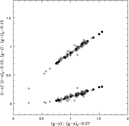
The red GCs in the inner regions of NGC 4486 show a peak at (g − z)ACS = 1.40 (or (g − z)′ = 1.33; see FVF12) indicating that these clusters are as red as the reddest galaxies in Fig. 5. That is, we do not find a significant offset between the colours of the red GCs and the colours of the galaxies as found by Goudfrooij & Kruijssen (2013). In addition, the bluest galaxies in this figure are bluer than the GCs with the lowest metal abundance. All of them show blue colour gradients towards their centres indicating recent star-forming processes.
6 PARAMETERS INFERRED FROM THE GALAXY COLOUR AND BRIGHTNESS FITS
We start by iterating the δ parameter until the model matches the composite integrated colours of the fiducial galaxies within one effective radius. A comparison of these (reddening corrected) colours with those corresponding to the whole galaxy does not show significant differences.
Then, Γ was changed until the absolute Mg magnitude of the models coincide with the observed ones. Remarkably, the mean δ for all galaxies exhibits a relatively low dispersion around the mean values (δ = 1.92 ± 0.13), very similar to that derived by FVF12 in their analysis of the galactocentric colour gradient observed in NGC 4486 (δ = 1.8). In turn, Γ is also almost constant for galaxies fainter than the ‘gap’ in the colour–magnitude diagram, yielding a mean value Γ = 0.72 ± 0.16 (in 10−9 units). Instead, the two brightest fiducials show an increase of this parameter with stellar mass as shown in Table 4.
Model results for the fiducial galaxies.
| Fiducial | Γa | log (Mhalo) | log (Mbulge) | log (Mb) | log (t) | log (tb) | log (tr) | log (Sm) | (M/L)B | [Z/H] |
|---|---|---|---|---|---|---|---|---|---|---|
| 1 | 2.44 | 10.984 | 11.757 | 11.850 | 0.853 | 1.695 | 0.800 | −0.448 | 7.6 | −0.15 |
| 2 | 1.09 | 10.343 | 11.196 | 11.253 | 0.556 | 1.187 | 0.232 | −0.899 | 7.1 | −0.27 |
| 3 | 0.59 | 9.981 | 10.903 | 10.952 | 0.300 | 0.938 | 0.079 | −1.198 | 6.8 | −0.32 |
| 4 | 0.53 | 9.760 | 10.586 | 10.646 | 0.283 | 0.883 | 0.027 | −1.179 | 6.8 | −0.32 |
| 5 | 0.67 | 9.421 | 10.354 | 10.402 | 0.383 | 0.993 | 0.192 | −1.217 | 6.6 | −0.38 |
| 6 | 0.61 | 9.502 | 9.997 | 10.118 | 0.525 | 0.929 | 0.233 | −1.102 | 5.8 | −0.57 |
| 7 | 0.76 | 9.121 | 9.518 | 9.664 | 0.767 | 1.134 | 0.436 | −0.902 | 5.2 | −0.73 |
| 8 | 0.88 | 9.049 | 9.065 | 9.358 | 1.010 | 1.206 | 0.713 | −0.702 | 4.5 | −1.03 |
| 9 | 0.98 | 8.853 | 8.765 | 9.113 | 1.077 | 1.244 | 0.712 | −0.605 | 3.9 | −1.06 |
| 9b | 0.75 | 9.057 | 0.000 | 9.057 | 1.130 | 1.130 | – | −0.605 | 3.9 | −1.46 |
aΓ in 10−9 units.
bMasses derived adopting δ = 1.9.
For the three brightest fiducials, we explored different models by changing both the Zsb and Zsr parameters, and the ratio of blue to red GCs. The most significant change is that, adopting an equal number of blue and red GCs outside the areas covered by the ACS field, the mass of the low-metallicity haloes decreases between 30 and 15 per cent.
The model colours of the fiducial galaxies corresponding to a single mean parameter δ = 1.9 are shown in Fig. 6 (where open dots represent the fiducial galaxies and filled dots correspond to the model fits) and are also presented in Table 1. In this figure we add 0.13 mag to our modelled colours in order to keep the same colour scale as in Fig. 1. The mean difference between observed and modelled colours for all the fiducials is −0.012 ± 0.04 mag. We stress that this rms value is coherent with the overall photometric errors. This figure also shows the effect of changing the δ parameter (as horizontal bars) from 0.5 to 2 times the adopted value and correspond to d(g − z)/d(log (δ) ≈ 0.18–0.10 (for the most and least massive galaxies, respectively). This shallow dependence of the model galaxy colours with δ is a consequence of the shapes of the distribution of the integrated stellar brightness with chemical abundance (or colour). For the range of Zs parameters that characterize a given GC population, these distributions are broad and bell shaped. A variation of δ (for a given Zs value) changes the skewness of these distribution, but has a relatively low impact on the mean colour. This situation also leads to the need to define fiducial galaxies since their mean colours are less affected by photometric errors, and also decrease the effect of particular star-forming events within a given individual galaxy.
Colour–magnitude diagram for the composite fiducial galaxies (open dots) compared with the colour modelling explained in the text (filled dots), corresponding to a single parameter δ = 1.9. The solid line has the same meaning as in Fig. 1. The overall colour rms resulting from the observed versus modelled colours is ±0.04 mag. The horizontal lines show the effect of changing the δ parameter from 0.95 to 3.80.
The halo, bulge-like and total composite masses obtained through the modelling procedure are given in Table 4.
The trends of the GC chemical scale lengths Zs with total stellar mass are depicted in Fig. 8 for each GC subpopulation. Red GCs exhibit a marked variation in comparison with the more shallow increase corresponding to the blue GCs. The Zs parameters of the three most massive fiducials are upper values as they come from the innermost regions of these objects. In this figure, and as a reference, we show the range covered by the Zs values of both subpopulations, as a function of galactocentric radii, in NGC 4486 (from FVF12).
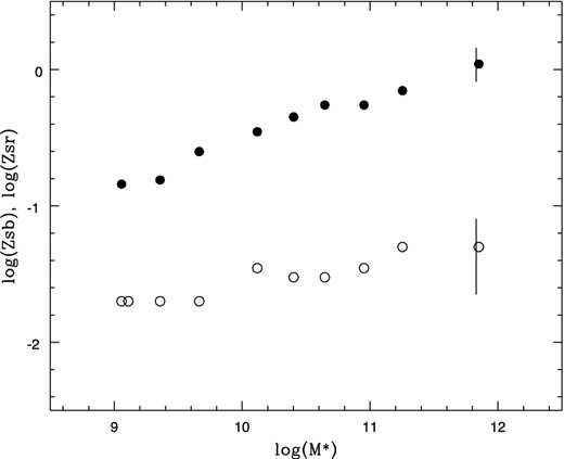
Chemical scale lengths corresponding to the red GCs (filled dots) and blue ones (open dots) as a function of the total stellar galaxy mass corresponding to the fiducial galaxies. The scale lengths of the three most massive galaxies are upper values derived for the central regions of these objects. Note that red clusters appear above log (M*) = 9.25 and exhibit a much evident change with stellar mass than their blue counterparts. The vertical lines represent the variation of these parameters with galactocentric radius in NGC 4486 (FVF12).
The behaviour of the chemical scale length of the blue GCs with galaxy mass (or luminosity) is consistent with a fact already pointed out by Strader, Brodie & Forbes (2004) in the sense that these clusters seem ‘to know’ about the galaxy they are associated with.
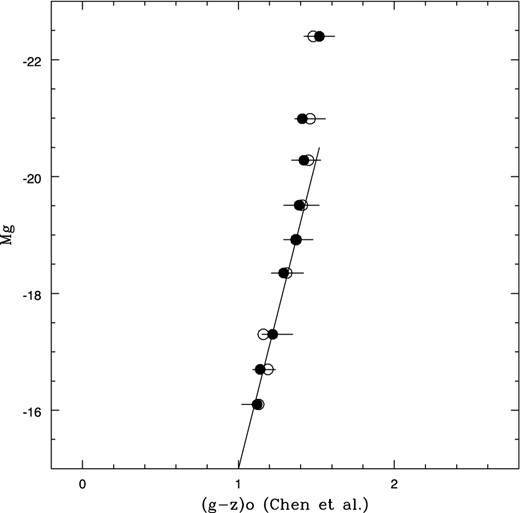
The composite (B-band luminosity weighted) chemical composition [Z/H] is displayed in Fig. 9. This diagram shows that a single power law does not yield a proper representation over the whole range of stellar mass and rather exhibits a smooth roll-over.
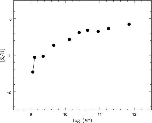
Inferred integrated chemical abundance (weighted by B-band luminosity) as a function of total stellar mass for each fiducial galaxy. Two possible models for the fiducial galaxy number 9 (see text) are shown connected by a line.
A single power law does not seem either an appropriate fit for the variation of the mass to luminosity ratio (M/L)B as seen in Fig. 10. This relation is in good agreement with the results presented by Tortora et al. (2009), through a completely different approach, and also with the mass to g-luminosity ratios derived by Kauffmann et al. (2003) and Bell et al. (2003; see their figs 14 and 6, respectively).
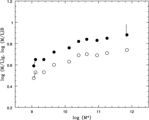
Inferred B-band (filled dots) and g-band (open dots) luminosity to stellar mass ratios as a function of stellar mass for all the fiducial galaxies. The ratios corresponding to the three most massive galaxies represent upper limits corresponding to the central regions of the galaxies. The vertical line at the right shows the galactocentric variation determined by FVF12 in the case of NGC 4486.
As illustrative examples, Fig. 11 displays the stellar mass distribution (normalized by total mass) inferred for the fiducial galaxies number 1, 6 and 9 on the basis of the parameters listed in Table 2. Note that, for the most massive object, the stellar distribution corresponds to its inner region and resembles the observed one for resolved stars in NGC 5128 (Harris & Harris 2002; Rejkuba et al. 2011), i.e. a broad and asymmetric high-metallicity (bulge-like) component and an extended low-metallicity tail. In the case of the least massive fiducial galaxy (number 9) we show an alternative distribution assuming that this galaxy only has blue GCs.
![Inferred chemical abundance distributions for the stellar populations in the fiducial galaxies number 1 (solid line), 6 (long dashed) and 9 (short dashed) normalized by mass and convolved with a Gaussian kernel (σ = 0.20 dex in [Z/H]). This figure also includes the expected distribution for the case of a bulgeless galaxy comparable to this last fiducial (long-short-dashed line).](https://oup.silverchair-cdn.com/oup/backfile/Content_public/Journal/mnras/441/2/10.1093/mnras/stu658/2/m_stu658fig11.jpeg?Expires=1716558823&Signature=UtbjF-yYNukRfMERbjrKFQDOqb9lTlIZ7qgBDIEZiMYE~066nvgQ1g18SaukAclarPuJ13EwhL2DV2aWiBwF84tUY73dQ1AKx6LTx~dMO41mLo9w7drN0FT4wb~tyl5oaiXoRNo6omQbtTqlFilzOxRCF4i47LtLwJv44S19gLu-wR8uBd8nUWEVO6IIm6wQT~RvGVrsw3gVwpdk7Py~bT2LyI0UoqIO20K4bXX6Fw6ELDghBntPW5lKpLzmCpsMKFZkD2vKVhCGk4FzmRITU~2tU---l-1bOh9FVrRrT2MzDlKJVVlJxM01UQ66pcrSxEg76ye0RFHp8AgROwHnEw__&Key-Pair-Id=APKAIE5G5CRDK6RD3PGA)
Inferred chemical abundance distributions for the stellar populations in the fiducial galaxies number 1 (solid line), 6 (long dashed) and 9 (short dashed) normalized by mass and convolved with a Gaussian kernel (σ = 0.20 dex in [Z/H]). This figure also includes the expected distribution for the case of a bulgeless galaxy comparable to this last fiducial (long-short-dashed line).
We use the term ‘resembles’ since a more thorough comparison will require a detailed analysis of the metallicity scales (and the different inherent errors) adopted in this and other works. In this last figure, the chemical abundances of the model have been convolved with a Gaussian kernel (with σ = 0.20 dex) in a preliminary approach to assess the effects of such errors. For example, these errors smooth-out the eventual presence of ‘valleys’ in the chemical abundance distributions arising as the result of combining halo and bulge components.
The integrated colour of the last fiducial (on our photometric scale) is (g − z)0 = 0.99 or (C − T1)0 = 1.32 (from the relations given in F13) and, then, (B − V)0 = 0.72, which after adding an interstellar colour excess E(B − V) = 0.02 leads to (B − V) = 0.70, a colour coincident with the photometric results given by Mihos et al. (2013) for the outer region of NGC 4472. This coincidence may indicate that galaxies with comparable, or with lower masses, can be the principal contributors to the formation of the low-metallicity haloes.
7 THE NUMBER OF GLOBULAR CLUSTERS VERSUS GALAXY MASS RELATION
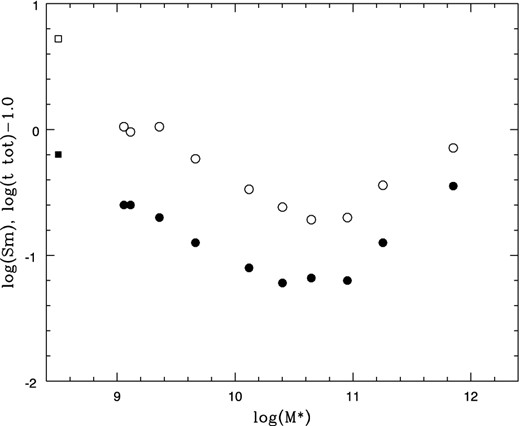
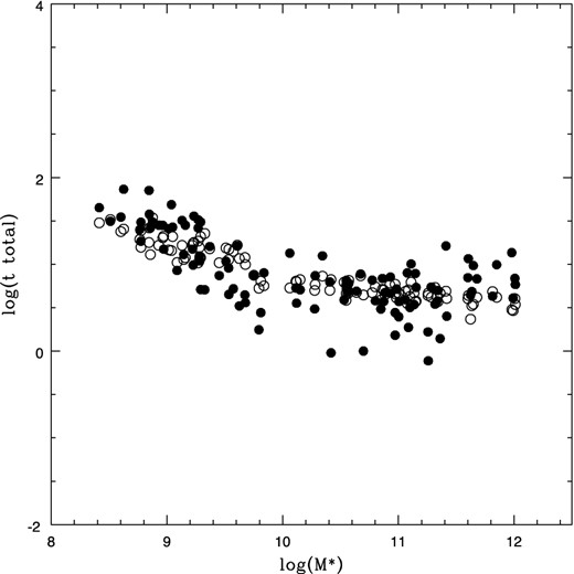
The total number of GCs was used to derive the ‘GC formation efficiency’ (i.e. number of GCs per stellar mass unit), t (in 10−9 units), and also Sm, the GC mass fraction content of each galaxy, as defined in HHA13. To derive this last parameter we adopted their power-law approximation to obtain the mean GC mass as a function of the stellar mass of the galaxy. Both t and Sm are displayed in Fig. 12. These parameters exhibit trends similar to those obtained by HHA13 (see their fig. 14).
The mean number of blue and red GCs for each fiducial galaxy is shown in Fig. 13. An interesting feature in these diagrams is that below log (M*) ≈ 11.0, where completeness factors do not play an important role, the slopes that characterize the increase of the number of blue and red GCs with total stellar galaxy mass are significantly different (0.30 ± 0.03 and 0.70 ± 0.02, respectively).
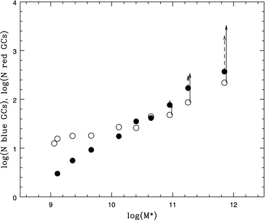
Number of blue GCs (open dots; solid lines) and red GCs (filled dots; dashed arrows) as a function of total stellar mass of each fiducial galaxy. The arrows indicate a tentative correction due to incomplete areal coverage (see text).
Alternatively, combining the number of blue and red GCs leads to the behaviour displayed in Fig. 14 corresponding to the total GC population. This diagram also supports the claim of HHA13 in the sense that the number of GCs is not a good indicator of the stellar mass of the galaxy. The straight line in this diagram has the same slope of the fit shown by these authors in their fig. 9. Thus, the behaviour pointed out by HHA13 is consistent with the presence of two distinct GC populations.
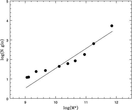
Total number of GCs (blue and red, added) as a function of the fiducial galaxy stellar masses. The straight line has the slope determined by HHA13. This diagram shows that a linear log–log approximation, as suggested by these authors, in fact is not a good representation of the number of clusters–galaxy stellar mass relation.
8 THE SÉRSIC INDEX AND THE PROJECTED STELLAR MASS DENSITY
Table 5 gives the Sérsic n index and the surface stellar mass density Σ (in M⊙ kpc−2) for the fiducial galaxies. The first parameter is just a mean value for the galaxies contained with each fiducial group as given by Chen et al. (2010). In turn, Σ was estimated by taking the mean surface brightness in the g band within one effective radius (mag arcsec−2) (table 2 in Chen et al. 2010), transforming this magnitude to B magnitudes (through the relations given in Section 2), and averaging all the galaxies within a given fiducial group. Finally, adopting the Mei et al. (2007) distance moduli, and the mass to B-band luminosity ratios given in Table 4, these surface brightnesses were transformed to M⊙ kpc−2. The relation between n and log (Σ) is shown in Fig. 15.
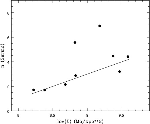
Sérsic n index versus surface stellar density Σ (in M⊙ kpc−2) obtained as explained in the text. A linear fit gives a good approximation for most fiducial galaxies except the two brightest ones.
Sérsic's parameter n and projected stellar mass density Σ (in M⊙ kpc−2) for the fiducial galaxies.
| Fiducial | log(n) | log (Σ) |
|---|---|---|
| 1 | 0.746 | 8.82 |
| 2 | 0.840 | 9.18 |
| 3 | 0.650 | 9.37 |
| 4 | 0.645 | 9.59 |
| 5 | 0.505 | 9.47 |
| 6 | 0.459 | 8.83 |
| 7 | 0.231 | 8.38 |
| 8 | 0.332 | 8.68 |
| 9 | 0.233 | 8.22 |
| Fiducial | log(n) | log (Σ) |
|---|---|---|
| 1 | 0.746 | 8.82 |
| 2 | 0.840 | 9.18 |
| 3 | 0.650 | 9.37 |
| 4 | 0.645 | 9.59 |
| 5 | 0.505 | 9.47 |
| 6 | 0.459 | 8.83 |
| 7 | 0.231 | 8.38 |
| 8 | 0.332 | 8.68 |
| 9 | 0.233 | 8.22 |
Only the two brightest galaxies appear well off, as seen in similar diagrams (e.g. Graham & Guzmán 2003). This figure shows an increase of n from ≈1.8 to ≈4, i.e. the fiducial galaxy profiles become more de Vaucouleurs-like as the projected stellar mass density increases.
Both n and Σ are displayed as a function of total stellar mass (in logarithmic format) in Fig. 16. This diagram shows the well known increase of n with galaxy mass and brightness (see e.g. Donofrio et al. 2011). In turn, the projected surface stellar mass increases until reaching a well defined peak at log (M*) ≈ 10.5 and an almost symmetric decrease for the brightest fiducials (i.e. for galaxies above the gap in the colour–magnitude diagram). This diagram is in fact a transformed version of fig. 1 in Kormendy et al. (2009), and the peak of the Σ value would be the boundary that, according to these authors, indicates a ‘dichotomy’ in the galaxy-forming process.
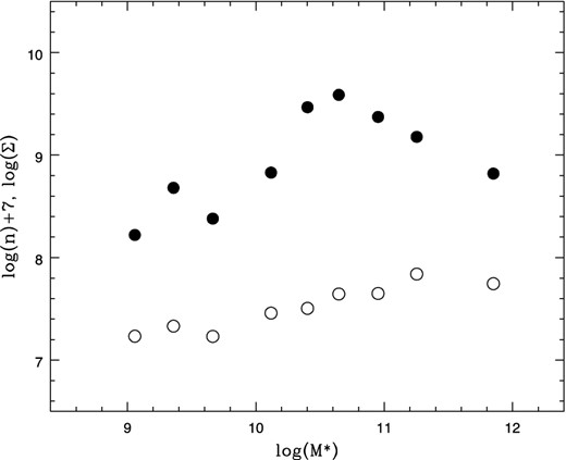
Variation of the logarithm of the Sérsic n index (shifted by +7; open dots) and projected stellar mass density with total stellar mass of the fiducial galaxies (solid dots). There is a marked peak at log (M*) ≈ 10.5 and then a decrease with increasing stellar galaxy mass.
9 HALO AND BULGE MASSES AND THEIR GLOBULAR CLUSTER FORMATION EFFICIENCIES
The dependences of the mass of the low-metallicity stellar halo (shifted by +7; open circles) and that of the bulge-like component (filled circles) with total stellar mass, as well as their respective mass fraction contribution, are displayed in Figs 17 and 18. The bulge-like component rises rapidly with galaxy mass, reaching 50 per cent at log (M*) ≈ 9.3 and about 85 per cent in the three highest mass fiducials. In the low-mass galaxies, the Zsr parameters are low, i.e. the corresponding red GCs are in fact rather blue (although we identify them as ‘red’ as a consequence of the working definition we adopted).
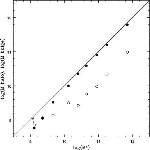
Variation of the bulge stellar mass associated with the red globulars (filled dots), and that corresponding to the low-metallicity stellar halo connected with the blue globulars (open dots). The straight line is the 1:1 relation.
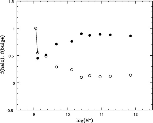
Fraction of low-metallicity halo (open dots) and bulge-like stellar population (solid dots) as a function of total stellar mass of the fiducial galaxies. Red globulars were not detected in the lowest mass galaxy (log (M*) ≈ 9.0). Note that the fractions of halo and bulge stellar masses are almost equal at log (M*) ≈ 9.3.
The GC formation efficiency, t, was defined in terms of the total stellar mass. The next step imply the definition of an ‘intrinsic’ t parameter, i.e. the number of GCs per stellar unit mass of the associated (halo or bulge) component. These tb or tr parameters are depicted as a function of the halo or bulge stellar masses in Fig. 19. Both GC subpopulations show a similarity in the sense that these parameters exhibit U-shaped forms and reach minimum values in the range defined by the fiducial galaxies number 4 and 5.
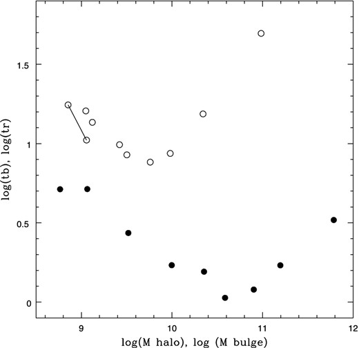
Intrinsic GC formation efficiencies tb (open circles) or tr (filled circles) as a function of the stellar masses of the halo or the bulge. Red globulars exhibit a marked minimum at log (M*) = 10.5, coincident with the peak of the stellar surface density Σ. Both GC subpopulations reach minimum values of their t parameters around the fiducial galaxy number 4.
An intriguing difference is shown in Fig. 20. In this figure, the red GCs (filled dots) show a clear anticorrelation with log (Σ) which is practically absent for the blue GCs. This behaviour is explained by the dominant role of the bulge-like component (connected with the red GCs) in terms of the mass of the projected stellar density Σ. In general, a dependence of the t parameter with both galaxy mass and Σ may be expected.
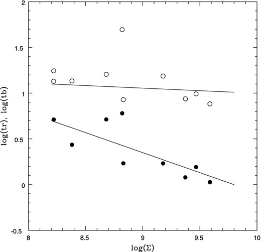
Intrinsic GC formation parameters tb for the blue (open dots) and tr for the red GCs (filled dots) as a function of the stellar surface mass density Σ. Both cluster families show a distinct behaviour. There is a clear trend shown by the red clusters whose tr parameters decrease with increasing Σ. In turn, blue globulars show a marginal variation and a larger dispersion of their tb parameters. The highest value, tb = 1.63, corresponds to the fiducial galaxy with the highest mass (number 1).
Total GC formation efficiency versus stellar mass for a sample of 126 E and S0 galaxies from HHA13 (filled dots). Open dots show the projection of these galaxies on the plane defined by the stellar mass and the projected stellar mass density Σ (see text).
10 DARK MATTER: WITH OR WITHOUT YOU?
The connection between GCs and DM haloes has been suggested in a number of papers in the literature (e.g. Blakeslee 1999; McLaughlin 1999; Spitler et al. 2008; Spitler & Forbes 2009; Georgiev et al 2010; HHA13). A still problematic issue in this kind of analysis is the wide range of values concerning the ratio between dark halo mass and stellar mass. Fig. 22 compares different results and is illustrative of this situation. The data correspond to Shankar et al. (2006), Berhoozi, Conroy & Weschler (2010), Leauthaud et al. (2012; values for redshifts lower than 0.1, compiled in their fig. 10) and HHA13. In this last case, the authors adopt a parametric approximation that assumes a constant ratio of the total stellar mass in GCs to dark halo mass, η = 6 × 10⁻⁵.
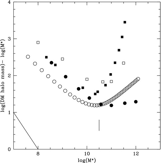
Comparison of the dark mass to stellar mass ratio from different sources. Filled dots: Shankar et al. (2006); filled squares: Berhoozi et al. (2010); open squares: Leauthaud et al. (2012; see text); open dots: HHA13. The line at left shows the effects of errors on stellar masses. The vertical line is an approximate position of a common minimum for all these ratios at log (M*) = 10.5.
Despite the differences between these relations, they have two common features: on one side, the slopes are very similar for stellar masses below log (M*) ≈ 10.5. On the other, all of them exhibit a more or less evident minimum at this last mass. Leauthaud et al. (2012) identify this minimum as a ‘pivot mass’ that changes with redshift but keeps a constant dark to stellar mass ratio ≈27.
That choice is motivated by two arguments. First, Fig. 23 shows a remarkable similarity between the dark to stellar mass ratios from these authors (scaled down by −2.07 in the logarithmic ordinate), and the ratio between the mass of the low-metallicity haloes to total stellar mass from Table 4. Moreover, recent studies of the giant elliptical galaxy NGC 5846, presented by Napolitano et al. (2014), and for NGC 4486, by Agnello et al. (2014), give a range of values of the dark halo to stellar mass ratios that are in excellent agreement with the Shankar et al. (2006) ratios.
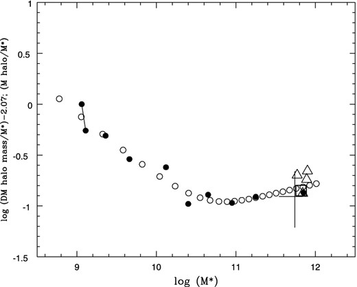
DM mass to total stellar mass ratio from Shankar et al. (2006; open circles), values for NGC 5846 from Napolitano et al. (2014; open triangles), and for NGC 4486 from Agnello et al. (2014; cross). All of them shifted vertically by −2.07 in ordinates. Low-metallicity halo mass to total stellar mass ratio for the fiducial galaxies are shown as solid dots. The open square represents the low-metallicity halo to total stellar mass in NGC 4486 (based on FVF12).
Secondly, this is consistent with previous results based on the similarity of the spatial distributions of the blue GCs and low-metallicity haloes and that of DM in NGC 1399 and NGC 4486 (FFG05 and FVF12, respectively). The shift of the Shankar et al. (2006) relation in Fig. 23 corresponds to stellar masses of ≈0.8 × 10⁻² of the dark halo mass. This is comparable to the ratio derived for NGC 4486, by combining the mass of the low-metallicity halo given in FVF12 (0.95 × 10¹¹ M⊙), and the total enclosed mass within about 100 kpc from Gebhardt & Thomas (2009) and Murphy, Gebhardt & Adams (2011) (1.3 × 10¹³ M⊙), that yield a ratio ≈0.5 × 10⁻².
Although these coincidences are encouraging for further analysis, we also note the discrepancy, pointed out by Strader et al. (2011), between different estimates of the dark halo mass in NGC 4486. Eventually, the adoption of the Shankar et al. (2006) relation, and our galaxy stellar masses, can be used to obtain the dark mass content for each fiducial galaxy, and for the definitions of tdark, tb dark and tr dark, i.e. the ratios between the number of total, blue and red GCs to DM mass.
Fig. 24 shows the behaviour of tdark as a function of the dark halo mass and the contribution of each GC subpopulation to this quantity. Blue and red clusters show opposite trends in the dark mass range from log (Mdark) = 11.0 to 12.0 (i.e. galaxies fainter than the ‘gap’ in the colour–magnitude diagram of Fig. 23), that once combined, lead to a rather constant tdark in that mass domain.
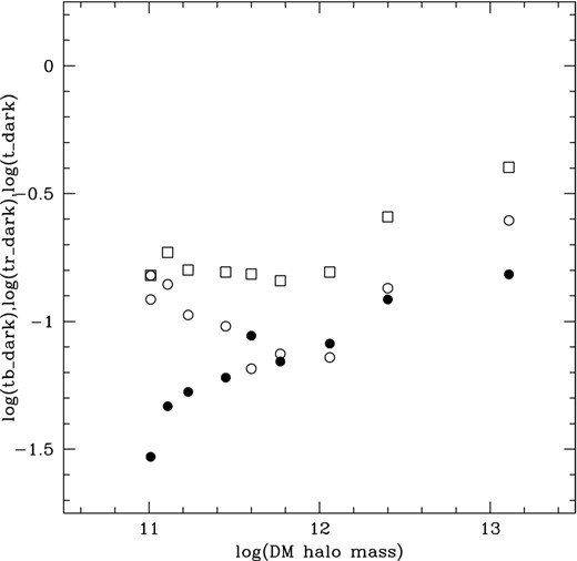
Number of GCs per unit dark mass for the blue (open circles), red (filled circles) and total population of GCs per unit dark mass (open squares) as a function of dark halo mass.
Fig. 25 compares the number of blue GCs per low-metallicity halo mass and per DM mass. These two parameters show similar trends (as expected if the low-metallicity halo and dark mass halo keep a constant ratio, as shown in Fig. 23). The minimum values in both tb and tb dark occur at the fourth fiducial galaxy, where the surface stellar density Σ reaches a maximum.
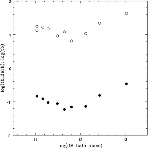
Number of blue GCs per low-metallicity halo mass (open circles) and unit dark mass (filled circles) as a function of dark halo mass.
This trend contrasts with the counterpart corresponding to the red GCs, shown in Fig. 26. In this case, the number of GCs per dark mass units increases along with the mass of the dark halo, showing an inflection at log (DM halo mass) ≈ 12.0. Instead, the tr parameter shows a minimum at a value coincident with the mass of the galaxies where the surface stellar density Σ reaches a maximum.
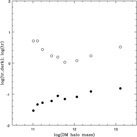
Number of red GCs per bulge mass (open circles) and unit dark mass (filled circles) as a function of dark halo mass.
For dark halo masses larger than log (Mdark) ≈ 12.2, both tr and tr dark rise in similar ways, although this is a consequence of our adopted approach regarding the distribution of blue and red GCs in the extended haloes of the three most massive fiducial galaxies. Fig. 27 shows that the Γ parameter listed in Table 4, scales very well with tdark (through a shift of −0.65 in the logarithmic ordinate). This connection suggests that the proportionality coefficient Γ may be an indication of the number of eventual GC formation sites (dark minihaloes) which will be occupied by blue or red GCs, depending on the availability of baryonic matter and its density (in turn associated with chemical abundance).
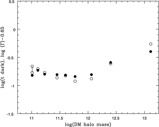
log (Γ), shifted by −0.65 (open circles), and log (tdark) parameters (filled circles) as a function of dark halo mass for each fiducial galaxy.
Finally, we note that Wu & Kroupa (2013) have a completely different view of the situation in the frame of Milgromian mechanics. These authors argue that the Sn parameter has two, and opposite, dependencies upon the apparent virial mass (including a ‘phantom’, i.e. non-existent dark halo) that, combined, leads to the U-shaped relation with the stellar mass of the galaxy.
11 LOW-MASS GALAXIES: THE CASE OF THE FORNAX SPHEROIDAL GALAXY
The Fornax spheroidal galaxy is ∼20 times less massive than our lowest mass fiducial galaxy and has five GCs. Battaglia et al. (2006) detect the presence of several stellar populations (ancient, intermediate and young) with a strongly asymmetric metallicity distribution of the field stars, that peaks at [Fe/H] ≈ −1.0, and has an extended tail that reaches [Fe/H] ≈ −2.5. Larsen, Strader & Brodie (2012) emphasize that this distribution is clearly different, and seemingly could not be reconciled with that of the GCs. Four of these clusters have [Fe/H] in the range from −2.1 to −2.5, while the remaining one (Fornax 4) has a higher metallicity, [Fe/H] = −1.4.
Establishing a connection of GCs with field stars is clearly difficult on the basis of a few clusters and is certainly affected by stochastic effects. Besides, the star formation history of the Fornax dwarf seems rather complex (see e.g. de Boer et al. 2012). With these caveats in mind, we attempted the same approach used in this paper. We start with a blue GC population characterized by a parameter Zsb = 0.02, similar to those in the lowest mass fiducial galaxy, and change both the number ratio of blue to red GCs, as well as the Zsr and δ parameters, aiming at reproducing the observed chemical abundance distribution of the field stars.
This is accomplished by adopting Zsr = 0.13, a number ratio of blue to red GCs of 4, and δ = 4, i.e. about twice the value that gives a proper fit to the more massive fiducial galaxies. We have no information about the behaviour of the δ parameter for galaxies with masses below log (M*) ≈ 9 but an increase with decreasing galaxy mass, and stellar density, cannot be dismissed.
The chemical abundance stellar mass spectrum delivered by the model is depicted in Fig. 28 and shows a very good qualitative agreement with the distribution for stars displayed in fig. 1 of Larsen et al. (2012). This comparison assumes that the stellar mass contained in each chemical abundance bin scales directly with the number of stars in the same bin.
![Model chemical abundance mass spectrum for the stellar population in a Fornax-like dwarf galaxy convolved with a Gaussian kernel with a dispersion of 0.2 dex in [Z/H].](https://oup.silverchair-cdn.com/oup/backfile/Content_public/Journal/mnras/441/2/10.1093/mnras/stu658/2/m_stu658fig28.jpeg?Expires=1716558823&Signature=xDm30BANrdvww7l2H6Lwz4dvaXcBTTy-3O7-kmaZj8ZbcyY9gTcP3an-vgGJkbablwyhjVZ-SHtm1yqMlanuSo5Xr6mkeImsnpO~554LlBwXPZ5NL4t1IDfRxGJ4MOlHGpJ91450Bz6twdw2irHPB8nH~vK9iufgmTmScyPxhlGIHtTLo5lW2-ZxzwizNTZcuHtzeWQmBScwe3p8eomtC-27pk7y29WPXs4DnsvNf4G2Xou~eUYsG48czE202KOFuRi4A9mey-I~M8Dw2wnbk0utx4MemfBdfl~j3T5Oc2NFPQ76DaBi4iyyARU-kO6zAwWN1cn8GzGQUo5kJHsoOw__&Key-Pair-Id=APKAIE5G5CRDK6RD3PGA)
Model chemical abundance mass spectrum for the stellar population in a Fornax-like dwarf galaxy convolved with a Gaussian kernel with a dispersion of 0.2 dex in [Z/H].
Note that in the case of the Fornax galaxy we expect the presence of a single red GC that possibly did not form or that eventually could be identified with Fornax 4.
12 CONCLUSIONS
This paper revisits the connection between GCs and the stellar populations of 67 galaxies included in the ACS Virgo Cluster Survey (Côté et al. 2004). The main results are the following.
The definition of composite fiducial galaxies was useful in clarifying the quantitative connection between GCs and the stellar populations of the galaxies they belong to. These fiducial galaxies are just a representation of average properties that arise as a result of different ‘nature-nurture’ events that take place along the life of a galaxy. The possibility of reproducing the integrated colours of galaxies through the analysis of their GCs, and with a constant parameter δ (equation 5), strongly suggests the existence of a common mechanism that regulates the link between clusters and field stars. The value of that parameter indicates higher GC formation efficiency as metallicity decreases. This dependence may be indicating a background process connected with environmental conditions (through a metallicity–stellar density link) as noted in Section 9.
We stress that the proposed GCs–field stars link also gives a proper representation of the chemical distribution of field stars for low-mass galaxies (e.g. the Fornax dwarf spheroidal) although it requires higher δ values, something we cannot justify yet on observational basis.
The separation of GCs in two families, according to their respective chemical scale lengths Zs, shows that blue and red clusters increase their number with total stellar galaxy mass but with distinct behaviours. Once combined as a ‘single population’, the log (NGCs) versus log (M*) relation found for the Virgo ACS galaxies is consistent with the non-linear trend (in a log–log plane) pointed out by HHA13.
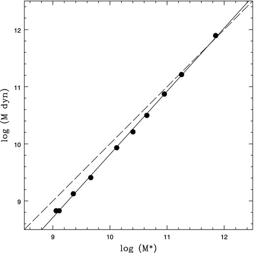
The mean total stellar mass of the fiducial galaxies follows a linear relation with the dynamical mass, given in terms of the stellar dispersion and effective radius presented by Wolf et al. (2010) and correlated with LV in HHA13.
The empirical approach proposed to connect GCs and field stars allows an estimate of the low-metallicity halo and bulge-like stellar masses. In particular, these last structures arise in galaxies with stellar masses larger than ≈109 M⊙ and grow up rapidly for more massive galaxies.
In this sense, they appear to be more ‘pseudo-bulges’ (originated in the ability of the galaxies to retain their chemical outputs) than bulges that grow as a consequence of environmental effects.
We also emphasize that bi-modality is a very solid feature since ‘dry merging’ of any of the bimodal fiducial galaxies ends up as a new, but also bimodal, GCs colour distribution, although with different Zsb and Zsr parameters.
The behaviour of the number of the blue or red GCs per stellar mass units of the populations they are respectively associated (halo or bulge-like) as a function of total stellar mass exhibits a similarity and a difference. On one side, they are both U-shaped and reach minimum values in the mass range defined by the fiducial galaxies 4 and 5. On the other, the red GCs show a marked (inverse) dependence with surface stellar mass density. This dependence is not detectable for the blue GCs as the total stellar mass is dominated by bulge-like stars.
The ratio of the low-metallicity stellar halo mass to total stellar mass exhibits a strong similarity (once properly normalized) with the ratio of total DM mass to stellar mass as presented in Shankar et al. (2006). In some way, the low-metallicity halo seems a kind of ‘subtle echo’ of the DM content if the dark to stellar mass ratios given by Shankar et al. (2006) are adopted.
It is intriguing that the increase of the Γ and tdark trends with galaxy mass occurs approximately at the so-called critical mass as defined by Dekel & Woo (2003), the mass value that suggests a ‘dichotomy’ in the galaxy formation process as argued by Kormendy et al. (2009), the ‘pivot’ mass defined by Leauthaud et al. (2012) and, as pointed out in this paper, the stellar mass where the projected stellar surface density Σ reaches a maximum value.
The reason for that increase is not clear although the dramatic change of the effective radii of these galaxies with brightness (and stellar mass), leading to low stellar densities, suggests that this kind of environments may favour the GCs formation efficiency (speculatively through better survivability conditions for the cooling flows where GCs would form).
In fact, the hierarchical models by Oser et al. (2010) indicate that the most massive galaxies, exhibit less in situ star formation, have less concentrated haloes, and also lower central densities. These authors also show that the size of these galaxies, and a large fraction of their masses, is the result of the accretion of objects formed ‘far’ from the central regions of the galaxies.
In our approach, the Zs scale lengths are a measurement of the spread of the metallicity of the blue GC/low-metallicity halo and of the red GC/bulge stars. The distinction between these ‘two’ components is in fact a ‘working definition’ in the sense that they provide a good match to the integrated galaxy colours. Even though the low-metallicity component is rather homogeneous and would be properly identified as a ‘single population’, this is not the case of the bulge-like component which, according to their larger Zs scales, suggests a rather inhomogeneous mix of stars with very different chemical abundances.
Forbes, Brodie & Huchra (1997) already suggested that GCs bimodality may be the result of a ‘two phases’ process. The meaning of ‘phase’, however, seems still an open issue in the context of some recent results. For example, several works point out that reionization has played a role (e.g. Elmegreen, Malhotra & Rhoads 2012; Spitler et al. 2012; Griffen et al. 2013; Katz & Ricotti 2013) in the formation of the metal-poor blue GCs that would appear at high redshifts and before the red (and more heterogeneous chemically) GCs. Tonini (2013; and also see Muratov & Gnedin 2010) gives arguments to support the existence of a discrete temporal sequence in the frame of hierarchical models, indicating that blue GCs form at a redshift of ≈4 and are later accreted by galaxies that already have their own metal-rich GCs (formed in situ) at redshifts of ≈2. This is similar to the scenario presented by Forte, Martinez & Muzzio (1982) for the particular case of NGC 4486 and later generalized by Côté et al. (1998). Tonini (2013) also concludes that red GCs only form in galaxies with stellar masses larger than 109 M⊙, in approximate agreement with the results presented in this paper regarding to these clusters and their associated bulge-like structures.
In contrast with that landscape, and as noted by Leaman et al. (2013; and also see VandenBerg, Brogaard & Leaman 2013) the results for the Milky Way GCs, rather than discrete events, show a continuous and bifurcated age sequence. These results indicate that both metal-poor and metal-rich GCs seem coeval and display the same range of ages (≈2 Gyr), although shifted in metallicity by ≈0.6 dex. In their view, blue GCs may need not to have formed in a truncated epoch and as separated episodes. A 2 Gyr difference between the low- (NGC 6397) and the high-metallicity (47 Tuc) Milky Way GCs is also found by Hansen et al (2013) on the basis of the study of the white dwarf sequences in these clusters.
In our analysis, we find that the chemical scale lengths of the blue GCs, Zb, slowly increase with total galaxy mass, i.e. at least a fraction of them have a link with these galaxies. In a tentative explanation, and coincident with Carretta (2013), we suggest that blue GCs may be a mix of clusters formed in situ (and showing a dependence with galaxy mass) and other accreted, more stochastically, from less massive fragments/galaxies.
If a bifurcated age sequence as in the Milky Way exists, the chemical abundances of both the blue and red GCs are genuine ‘in phase’ clocks. This would indicate that the term ‘phase’ (in the context of Forbes et al. 1997) is more a feature connected with environment than with time.
To the question posed by HHA13 regarding ‘what determines the size of a GC population?’, this paper suggests that it is a competing mechanism where the number of GCs depends on the availability of potential formation sites, that increases with galaxy mass and, at the same time, has an inverse dependence with stellar density.
As a final conclusion, we find support for the idea that GCs in fact codify information about the large-scale features of ETGs. However, the complete code is not yet conclusively understood.
We thank Dr William E. Harris for his interesting and helpful comments. JCF acknowledges the hospitality of Lic. Lucía Sendón (Director) of the ‘Galileo Galilei’ Planetarium (Buenos Aires). This work was supported by grants from CONICET (PIP-2009-0712) and from La Plata National University (G128), Argentina. AVSC acknowledges financial support from Agencia de Promoción Científica y Tecnológica of Argentina (BID AR PICT 2010-0410).
