-
PDF
- Split View
-
Views
-
Cite
Cite
Richard J. Parker, Morten Andersen, Spatial differences between stars and brown dwarfs: a dynamical origin?, Monthly Notices of the Royal Astronomical Society, Volume 441, Issue 1, 11 June 2014, Pages 784–789, https://doi.org/10.1093/mnras/stu615
Close - Share Icon Share
Abstract
We use N-body simulations to compare the evolution of spatial distributions of stars and brown dwarfs in young star-forming regions. We use three different diagnostics: the ratio of stars to brown dwarfs as a function of distance from the region's centre, |$\mathcal {R}_{\rm SSR}$|, the local surface density of stars compared to brown dwarfs, ΣLDR, and we compare the global spatial distributions using the ΛMSR method. From a suite of 20 initially statistically identical simulations, 6/20 attain |$\mathcal {R}_{\rm SSR} \ll 1$| and ΣLDR ≪ 1 and ΛMSR ≪ 1, indicating that dynamical interactions could be responsible for observed differences in the spatial distributions of stars and brown dwarfs in star-forming regions. However, many simulations also display apparently contradictory results – for example, in some cases the brown dwarfs have much lower local densities than stars (ΣLDR ≪ 1), but their global spatial distributions are indistinguishable (ΛMSR = 1) and the relative proportion of stars and brown dwarfs remains constant across the region (|$\mathcal {R}_{\rm SSR} = 1$|). Our results suggest that extreme caution should be exercised when interpreting any observed difference in the spatial distribution of stars and brown dwarfs, and that a much larger observational sample of regions/clusters (with complete mass functions) is necessary to investigate whether or not brown dwarfs form through similar mechanisms to stars.
1 INTRODUCTION
One of the outstanding questions in star formation is whether the mechanism through which brown dwarfs (BDs, objects not massive enough to burn hydrogen in their cores) form is more like that of higher (e.g. solar) mass stars, or more like that of giant planets. This can be addressed by comparing the various properties of BDs with stars, such as multiplicity (Duchêne & Kraus 2013), kinematics (Luhman et al. 2007), and spatial distribution (Kumar & Schmeja 2007).
Several studies (e.g. Luhman 2006; Bayo et al. 2011; Parker et al. 2011; Parker, Maschberger & Alves de Oliveira 2012) have shown that BDs have a similar spatial distribution to stars in some star-forming regions; but there are other regions where the BDs appear to be more spread out (Kumar & Schmeja 2007; Caballero 2008; Kirk & Myers 2012). Furthermore, several studies (Andersen et al. 2011; Suenaga et al. 2013) have determined the ratio of stars to BDs (the ‘substellar ratio’ |$\mathcal {R}_{\rm ss}$|) as a function of distance from the centre of the Orion Nebular Cluster (ONC) and there is tentative evidence for a decrease in |$\mathcal {R}_{\rm ss}$| as a function of distance from the cluster centre, though measuring the substellar mass function in this region (and others) remains challenging (e.g. Alves de Oliveira et al. 2012; Da Rio et al. 2012; Lodieu et al. 2012).
Taken at face value, these results suggest that BDs have different spatial distributions to stars in some (but not all) star-forming regions and clusters. This could imply that BDs form through a different mechanism to stars in those regions (e.g. Thies & Kroupa 2008), or perhaps that dynamical interactions alter their spatial distribution in some regions (e.g. Reipurth & Clarke 2001; Adams et al. 2002; Goodwin et al. 2005), but not others. In order to test this, N-body simulations (which can be repeated many times with different random number seeds to gauge the level of stochasticity in the initial conditions) of the evolution of young star-forming regions should be analysed with the same method(s)/technique(s) used to analyse observational data.
In this paper, we use three different diagnostics to compare the spatial distributions of stars and BDs in numerical simulations of the evolution of star-forming regions. We measure the ratio of stars to BDs (|$\mathcal {R}_{\rm ss}$|) as a function of distance from the cluster centre; we compare the ‘local density ratio’ of stars and BDs using the ΣLDR method (Maschberger & Clarke 2011; Parker et al. 2014), and we compare the global spatial distributions using the ‘mass segregation ratio’ ΛMSR (Allison et al. 2009). We then re-examine the ONC data from Andersen et al. (2011) to look for differences in the local density of BDs compared to stars using ΣLDR, and the relative spatial distribution using ΛMSR.
2 QUANTIFYING DIFFERENCES BETWEEN STARS AND BROWN DWARFS
3 N-BODY SIMULATIONS
3.1 Initial conditions
In the following analysis, we use only one set of initial conditions for star-forming regions, which we deem to be the most dynamically extreme in terms of the number of ejections of, and the maximum density experienced by, the stars and BDs (Allison 2012).
The star-forming regions consist of 1500 objects, distributed randomly in a fractal with dimension D = 1.6 and radius rF = 1 pc. This fractal dimension results in a very clumpy distribution, which can lead to the ejection of low-mass objects from the clumps. However, the initial spatial distributions of stars and BDs are indistinguishable. The global virial ratio (defined as αvir = T/|Ω|, where T and |Ω| are the total kinetic energy and total potential energy of the stars, respectively) is αvir = 0.3, i.e. subvirial. For the exact details of the spatial set-up, and the velocity distribution of stars and BDs, we refer the interested reader to Goodwin & Whitworth (2004) and Parker et al. (2014).
We draw primary masses from the Maschberger (2013) formulation of the initial mass function (IMF). We then assign binary separations based on the primary mass (the mean separation decreases with decreasing primary mass; Burgasser et al. 2007; Bergfors et al. 2010; Raghavan et al. 2010; Janson et al. 2012; Sana et al. 2013; De Rosa et al. 2014) and mass ratios drawn from a flat distribution (Metchev & Hillenbrand 2009; Reggiani & Meyer 2011, 2013; Duchêne et al. 2013). Finally, eccentricities are drawn from a flat distribution (Abt 2006; Raghavan et al. 2010). This set-up results in a global system star-to-BD-ratio of 4:1, consistent with both the Galactic field and star-forming regions (Chabrier 2005; Andersen et al. 2008; Bochanski et al. 2010).
We evolve the star-forming regions for 10 Myr using the kira integrator in the starlab package (Portegies Zwart et al. 1999, 2001). We do not include stellar evolution in the simulations.
3.2 Dynamical evolution over 10 Myr
The evolution of the star-forming regions follow the same qualitative pattern; substructure is erased within the first ∼1 Myr (Goodwin & Whitworth 2004; Allison et al. 2010; Parker & Meyer 2012) and the subvirial velocities lead to violent relaxation and collapse to a centrally concentrated, bound cluster (Parker & Meyer 2012; Parker et al. 2014). The adopted initial conditions lead to an ejected halo of objects on the outskirts of the cluster (Allison 2012). However, the evolution of other parameters is highly stochastic; some clusters exhibit mass segregation whereas others do not (Allison et al. 2010; Parker et al. 2014), and the binary population (both stars and BDs) can be altered to varying degrees (Parker & Goodwin 2012).
Because the cluster expands due to two-body interactions (Gieles, Moeckel & Clarke 2012; Moeckel et al. 2012; Parker & Meyer 2012), it is difficult to define a radially varying |$\mathcal {R}_{\rm ss}$| ratio for annuli of fixed physical width. For this reason, we adopt four annuli from the cluster centre-of-mass; 0–0.25 rc; 0.25–0.50 rc; 0.50–0.75 rc; and 0.75–0.95 rc, where rc is the total extent of the cluster in the N-body simulation. We exclude the very outskirts (>95 per cent) of the cluster – i.e. ejected stars, though we note that in future the Gaia satellite may be able to trace the birth sites of ejected BDs from clusters. We then compute the |$\mathcal {R}_{\rm SSR} = \mathcal {R}_{{\rm ss}, {\rm out}}/\mathcal {R}_{{\rm ss}, {\rm in}}$| ratio as the ratio of the outer annulus to the inner.
We determine ΛMSR for the 2D distribution within 95 per cent of the cluster centre at each simulation snapshot and compare the MST of the 50 lowest mass (<0.02 M⊙) objects to randomly chosen MST lengths. We choose 50 objects to strike a balance between having too few links in the MST (which would produce a very noisy signal), and too many (which would be washed out against the mean MST). We also determine the local density ratio ΣLDR for all BDs, compared to stars with masses less than 1 M⊙, again in two dimensions within 95 per cent of the cluster members.
We use the 95 per cent extent and perform our calculations in 2D to attempt to mimic the information available to observers. However, we also repeated the analysis in 3D for stars which are energetically bound to the cluster using the method outlined in Baumgardt, Hut & Heggie (2002), and in a very conservative calculation we repeated the original 2D determination but limited the extent to 85 per cent of the cluster. Both of these alternative determinations give very similar results to our default calculation.
In Fig. 1, we show the evolution of |$\mathcal {R}_{\rm SSR}$|, ΛMSR, and ΣLDR for 3 out of our suite of 20 simulations. In each panel, we plot a filled symbol when the deviation from unity is significant (more than 2σ) for each measure. In panel (b), we show the uncertainty associated with ΛMSR as defined by equation (2) for one simulation – the uncertainties on the remaining simulations are not shown because the plot would become unreadable, but are similar in size. The magnitude of the uncertainties associated with |$\mathcal {R}_{\rm SSR}$| and ΣLDR are also comparable.
Evolution of |$\mathcal {R}_{{\rm ss}, {\rm out}}/\mathcal {R}_{{\rm ss}, {\rm in}}$|, ΛMSR and ΣLDR with time for three individual simulations. For each measurement, we plot a filled symbol when the value significantly deviates from unity. In panel (b), we show the uncertainties on the ΛMSR measurements according to equation (2) for one simulation. |$\mathcal {R}_{{\rm ss}, {\rm out}}/\mathcal {R}_{{\rm ss}, {\rm in}} < 1$| indicates that more BDs are located on the outskirts of the cluster than in the centre, ΛMSR < 1 indicates that the BDs collectively have a more sparse spatial distribution, and ΣLDR < 1 indicates that the BDs have lower local density than more massive objects.
In the first simulation (the black lines/circles), the |$\mathcal {R}_{\rm SSR}$| ratio is actually significantly less than unity before dynamical evolution occurs (despite their spatial distributions being the same). This ratio rises to unity during the cool collapse, but then is significantly less than unity for the remainder of the simulation. This could be interpreted as the BDs being ejected into the outskirts of the cluster, and if this is the case we might expect them to have a more sparse spatial distribution than the stars. This is confirmed by the ΛMSR ratio, which shows the BDs to be more spatially spread out with respect to the average cluster members. Furthermore, the ΣLDR ratio shows that on average, the local surface density around BDs to be lower than for stars. Taken together, the natural interpretation is that dynamical interactions have ejected the BDs to the cluster periphery.
If we examine each simulation individually, we find that at various points in the whole 10 Myr of evolution, 6/20 simulations have |$\mathcal {R}_{\rm SSR} \ll 1$| and ΛMSR ≪ 1 and ΣLDR ≪ 1. The simulation shown by the black points/lines in Fig. 1 displays significant differences between the spatial distributions of stars and BDs in all three diagnostics for a total of 2.8 Myr, and significant differences in two of the three diagnostics for another 7.0 Myr in total. There are another five simulations which show differences in all three diagnostics, but for a much shorter total time: 0.4, 0.3, 0.1, 0.1, and 0.1 Myr. 14/20 simulations show significant differences in two of three diagnostics for some of their evolution (the median length is 0.5 Myr), and all simulations show a difference between the spatial distributions of stars and BDs in at least one diagnostic for some of their evolution (the median length is 2.7 Myr).
However, if we examine another simulation (the blue lines/squares), we see that the |$\mathcal {R}_{\rm SSR}$| ratio is significantly lower than unity in the first 2 Myr, before becoming more than unity (i.e. there are relatively more BDs than stars in the central region, compared to the outskirts). At the same time, ΛMSR suggests that the BDs are more spread out from 3 Myr onwards, whereas ΣLDR indicates that the BDs are not in regions of lower local density than the stars. In a third simulation (the red lines/triangles), neither |$\mathcal {R}_{\rm SSR}$| nor ΛMSR are significant, yet the ΣLDR ratio taken in isolation would suggest that the BDs are in locations of lower surface density than the stars.
In order to gauge the significance of these particular simulations, we plot the evolution of each of our chosen metrics for all 20 simulations in Fig. 2. The crosses indicate the median value from 20 simulations at each snapshot, whereas the black ‘error bars’ indicate the 25 and 75 percentiles, and the full range in the simulations is shown by the grey ‘error bars’. (Note that these are not error bars in the conventional sense – we are only showing the range of values from 20 simulations at a given time, and not the uncertainty on the measurement.) On average, each measurement does not significantly deviate from unity, suggesting that dynamical processing cannot be the mechanism which results in different spatial distributions of BDs compared to stars. However, as we have seen, using only one metric can lead to erroneous (or at the very least naïve) conclusions.
Evolution of |$\mathcal {R}_{{\rm ss}, {\rm out}}/\mathcal {R}_{{\rm ss}, {\rm in}}$|, ΛMSR and ΣLDR (BDs/stars) for all 20 simulations. Each panel shows the median value of 20 simulations with identical initial conditions (the crosses) and the darker ‘error bars’ indicate 25 and 75 percentile values. The entire range of possible values from the 20 sets of initial conditions is shown by the lighter ‘error bars’.
4 DATA FOR THE ONC
Given the difficulty in assessing whether any different spatial distribution of stars compared to BDs is an outcome of the star formation process, we revisit the data from Andersen et al. (2011) to assess whether the decreasing star to BD ratio in the ONC is also echoed in the ΛMSR and ΣLDR ratios. The data from Andersen et al. (2011) are not contiguous – the coverage consists of a mosaic of ‘postage stamp’-like fields which appear as strips placed across the cluster, so we must assume that the observed distribution of stars and BDs is also representative of that in the ‘missing’ data.
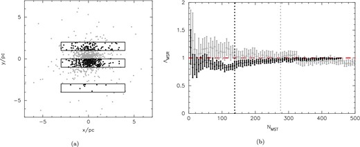
In order to test the performance of ΛMSR and ΣLDR on non-contiguous data, we create a Plummer (1911) sphere with 1000 stars drawn randomly from the Maschberger (2013) IMF and also positioned at random. These positions are shown by the grey points in Fig. 3(a). In Fig. 3(b), we show the ΛMSR measurement as a function of NMST for the BDs by the grey triangular points and their uncertainties. The location of the boundary between stars and BDs is shown by the right-hand vertical dotted grey line. Whilst the calculation is quite noisy for low NMST, the values are consistent with unity. We then draw strips on the cluster and repeat the analysis, restricting the sample to the 461 stars within these strips, but allow MST links between stars in different strips. The results are shown by the black circular points (and uncertainties) in Fig. 3(b) and the location of the boundary between stars and BDs is shown by the left-hand vertical dotted black line. Allowing MST links between the strips does give a small ‘depression’ in the progression of ΛMSR as a function of NMST, but the 60 lowest mass BDs have a ΛMSR consistent with unity. The ΣLDR value for the full sample is 1.08 (with a KS p-value 0.92), whereas the ΣLDR value for the restricted sample is 0.79 (with KS p-value 0.16). Therefore, in both samples the ratio is not significantly different from unity. We therefore conclude that the unusual geometry of the ONC data should not affect the determination of either ΛMSR or ΣLDR.
The effects of non-contiguous data on the ΛMSR analysis. In panel (a), we show the positions of 1000 stars in a Plummer sphere, and impose strips on the cluster to mimic the data in Andersen et al. (2011). In panel (b), we show the determination of ΛMSR as a function of the NMST least massive objects in the full sample (the grey triangular points/error bars) and for the restricted sample – the 461 stars within the strips (the black circular points/error bars). The left-hand (black) vertical dotted line shows the boundary between BDs and stars for the restricted sample, and the right-hand (grey) line shows the boundary location in the full sample. The red dashed line indicates ΛMSR = 1.
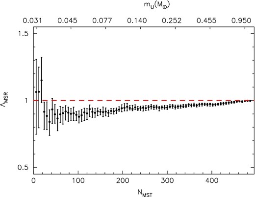
Using the data from Andersen et al. (2011), we first determine ΛMSR as a function of the NMST least massive objects in the observational sample as shown in Fig. 4. The data show a marginally more spread-out spatial distribution of the BDs compared to the cluster average, although the most extreme value is |$\Lambda _{\rm MSR} = 0.84^{+0.09}_{-0.10}$| for the 36 least massive objects, which is barely significant. ΛMSR = 1 (i.e. no mass segregation) is shown by the dashed line.
The evolution of the mass segregation ratio, ΛMSR, for the NMST least massive objects in the observational sample in Andersen et al. (2011). We indicate the highest mass star, mU within the NMST. Error bars show the 1/6 and 5/6 percentile values from the median. The dashed line indicates ΛMSR = 1, i.e. no mass segregation.
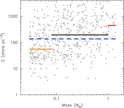
We also plot the local surface density Σ against object mass m in Fig. 5, using the surface densities calculated for the whole non-contiguous sample. The median surface density for BDs is |$\Sigma _{0.03 \le m/{\rm M_{\odot }} \le 0.08} = 56$| stars pc−2, shown by the horizontal orange line, compared to |$\Sigma _{0.08 < m/{\rm M_{\odot }} \le 1.0} = 196$| stars pc−2 for stars, shown by the horizontal black line (ΣLDR = 0.29). A KS test between the two distributions gives a p-value <10−7 that the two subsets share the same parent distribution.
The distribution of local stellar surface density, Σ, as a function of mass, m, for the objects in the observational sample in Andersen et al. (2011). The median surface density for the full sample is shown by the dashed (blue) line. The median surface density of BDs (0.03 ≤ m/M⊙ ≤ 0.08) is shown by the left-hand (orange) line; the median surface density of low-mass stars (0.08 < m/M⊙ ≤ 1.0) is shown by the middle (black) line and the median surface density of high-mass stars in the Andersen et al. observational sample (1.0 < m/M⊙ ≤ 1.4) is shown by the right-hand (red) line.
We also repeated the above analysis but limited the data to objects within 1 pc of the ONC centre and found similar results, suggesting that any field star contaminants in the data do not influence our analysis.
In tandem with the |$\mathcal {R}_{\rm SSR}$| ratio, ΛMSR and ΣLDR both suggest that the spatial distribution of BDs is different to stars in the ONC. However, this may not necessarily be a primordial signature of star formation, as we have seen in N-body simulations where 6/20 clusters have a dynamical evolution that leads to spatial differences between stars and BDs.
5 CONCLUSIONS
We have used three different diagnostics to look for differences in the spatial distributions of stars compared to BDs in N-body simulations of star-forming regions. We find that determining the |$\mathcal {R}_{\rm ss}$| ratio as a function of distance from the cluster centre cannot be used on its own to draw conclusions on the spatial distribution of BDs compared to stars. In a cluster with a radially decreasing |$\mathcal {R}_{\rm ss}$| ratio, the BDs may have a spatial distribution that is indistinguishable from stars (ΛMSR = 1, ΣLDR = 1).
Similarly, the inverse can also be true; the BDs have a significantly different spatial distribution compared to stars in that they are more spread out (ΛMSR ≪ 1 and/or ΣLDR ≪ 1), but the |$\mathcal {R}_{\rm ss}$| ratio increases or remains constant towards the outskirts of the cluster. These findings lead us to strongly advocate the use of more than one diagnostic when assessing the spatial distributions of BDs compared to stars in star-forming regions.
When applied to data from the ONC, the |$\mathcal {R}_{\rm SSR}$| ratio and ΣLDR ratio – and tentative evidence from ΛMSR – do suggest that the BDs are more spread out than stars. However, this data set is spatially incomplete, and a more comprehensive survey of the ONC would be highly desirable.
Randomly distributing masses drawn from an IMF can result (in 1/20, or 5 per cent, of simulations) in a radially decreasing |$\mathcal {R}_{\rm ss}$| ratio before dynamical evolution, which may or may not be mirrored in the ΛMSR and ΣLDR measurements. Furthermore, dynamical evolution leads to significant differences between the spatial distributions of stars and BDs in more than 25 per cent of our simulations. This implies that a large observational sample of regions/clusters is needed to assess whether the primordial spatial distributions of stars and BDs are different (which would suggest that their formation mechanisms are different).
We thank the anonymous referee for their comments and suggestions, which have improved the manuscript. The simulations in this work were performed on the BRUTUS computing cluster at ETH Zürich. RJP acknowledges support from the Swiss National Science Foundation (SNF). MA acknowledges support from the ANR (SEED ANR-11-CHEX-0007-01).


