Modelling [C i] emission from turbulent molecular clouds

Abstract

1 INTRODUCTION

Giant molecular clouds (GMCs) are the sites where the majority of Galactic star formation occurs, and hence it is important to understand their properties if we are to understand how star formation proceeds within our Galaxy. The two most abundant chemical species in molecular clouds are molecular hydrogen (H₂) and atomic helium, and between them they are responsible for the vast majority of the mass of the clouds. However, neither of these species can easily be observed within molecular clouds, as the gas temperature is too low to excite their internal energy levels. Observational studies of GMCs are therefore forced to focus on less abundant tracers that can be observed at typical GMC temperatures. The most popular such tracer is carbon monoxide (CO).¹

Unfortunately, CO is not without its problems as a molecular gas tracer. At high column densities, the problem is one of opacity: the CO rotational transitions start to become optically thick, breaking the relationship between CO emission and column density (see e.g. Pineda, Caselli & Goodman 2008). Fortunately, this problem can be avoided to a large extent by observing less common isotopic variants of CO, such as ¹³CO or C¹⁸O, which remain optically thin up to much higher column densities. At low column densities, on the other hand, the problem is one of abundance: in low extinction regions, CO is strongly photodissociated by the interstellar radiation field (ISRF), making it very difficult to observe any CO emission from these regions (see e.g. van Dishoeck & Black 1988; Goldsmith et al. 2008), let alone to learn anything about the thermal state or kinematics of this gas.

It is therefore worthwhile examining other possible tracers of the gas within molecular clouds. One particularly interesting possibility is neutral atomic carbon. Spin–orbit coupling splits the atomic carbon ground state into three fine structure levels with total angular momenta J = 0, 1, 2, and forbidden transitions between these three levels give rise to two prominent fine structures lines: the [C i] ³P₁ → ³P₀ transition at 609 μm (hereafter written simply as the 1 → 0 transition) and the [C i] ³P₂ → ³P₁ transition at 370 μm (hereafter the 2 → 1 transition). The energy difference between the ³P₁ and ³P₀ levels is only ΔE₁₀/k ≃ 24 K, while between the ³P₂ and ³P₀ levels it is ΔE₂₀/k ≃ 60 K. Therefore, at typical molecular cloud temperatures of 10–20 K, both of the fine structure lines can be excited.

So far, however, neutral atomic carbon has attracted much less attention than CO as a molecular cloud tracer. There are several reasons for this. Observationally, the [C i] lines are harder to study than the low J rotational transitions of CO: they typically have lower brightness temperatures, and are also situated in a wavelength regime where the effects of atmospheric absorption can be highly significant. Theoretically, it was originally thought that neutral atomic carbon would be abundant only at the edges of clouds (Langer 1976), limiting its usefulness as a tracer of the bulk of the cloud. Subsequent observations have shown that this expectation is incorrect, and that [C i] 609 μm emission is widespread within clouds (Frerking et al. 1989; Little et al. 1994; Schilke et al. 1995; Kramer et al. 2008), and yet the perception of [C i] as a tracer of cloud surfaces has proved difficult to shift.

In the past few years, however, there has been renewed interest in the prospects of [C i] as a molecular gas tracer. The CHAMP+ and FLASH instruments on the APEX telescope² have allowed both [C i] lines to be studied with reasonable sensitivity from one of the best sites on the planet, and ALMA³ will allow these lines to be studied with much greater sensitivity and angular resolution once bands 8 and 10 are commissioned. Moreover, in the longer term, CCAT⁴ will be able to rapidly map [C i] emission over large areas of the sky with good sensitivity. The time is therefore ripe for an in-depth look at what [C i] emission can tell us about molecular clouds, using state-of-the-art numerical simulations.

In this paper, we take the first steps towards this goal. We present results from a simulation of the chemical, thermal and dynamical evolution of a 10⁴ M_⊙ turbulent molecular cloud illuminated by the standard ISRF, and examine in detail how the neutral atomic carbon is distributed in this cloud. We also make synthetic emission maps of the resulting [C i] lines, and investigate how much we can learn about the cloud by looking at this emission. Although our focus in this paper is the detailed analysis of a single simulation, we plan to follow this up in future work with a much broader parameter study.

The plan of the paper is as follows. In Section 2, we present the numerical approach used to simulate the cloud and generate the synthetic emission maps. We also outline the initial conditions used for our simulation. Our main results are presented in Section 3, where we examine the chemical and thermal state of the gas in the cloud, and investigate what we can learn about the properties of the cloud from the [C i] emission. Finally, in Section 4 we present our conclusions.

2 METHOD

2.1 Hydrodynamical model

The chemical and thermal evolution of the gas in our model cloud is simulated using a modified version of the gadget 2 smoothed particle hydrodynamics (SPH) code (Springel 2005). Our modifications include a simplified treatment of the gas chemistry, based on the work of Glover & Mac Low (2007a,b) and Nelson & Langer (1999), and described in more detail in Glover & Clark (2012b), a detailed atomic and molecular cooling function (Glover et al. 2010), and a treatment of the attenuation of the ISRF within the cloud using the treecol algorithm (Clark, Glover & Klessen 2012a). The same code has previously been used to model star formation in molecular clouds with a variety of metallicities (Glover & Clark 2012c), the formation of GMCs from converging flows of atomic gas (Clark et al. 2012b), and the thermal state of the dense Galactic Centre molecular cloud known as the ‘Brick’ (Clark et al. 2013). More extensive discussions of the numerical details of the code can be found in these references. Here, in the interests of brevity, we focus only on a small number of changes that we have made to the code compared to the version described in these previous works.

The most important change that we have made involves our treatment of CO photodissociation. Previously, this was based on the work of Lee et al. (1996), but we have now updated our treatment to follow the recent paper by Visser, van Dishoeck & Black (2009). Comparison of runs performed with the old and new treatments of CO photodissociation demonstrates that the main difference in behaviour is a sharpening of the transition between regions dominated by neutral atomic carbon and regions dominated by CO, owing to the steeper dependence of the CO photodissociation rate on the visual extinction, A_V, found in the newer work.

2.2 Post-processing

We post-process our simulation data to produce synthetic emission maps in the ³P₁ → ³P₀ and ³P₂ → ³P₁ fine structure lines of [C i] and the J = 1 → 0 line of ¹²CO and ¹³CO using the radmc-3d radiation transfer code⁵, and making use of atomic and molecular data (transition energies, radiative transition rates, collisional excitation rate coefficients, etc.) from the LAMDA data base⁶ (Schöier et al. 2005). We calculate level populations using the large velocity gradient (LVG) approximation, as described in Shetty et al. (2011a,b). radmc-3d cannot presently deal with SPH data directly, and so before we can use the code to generate our synthetic emission maps, we must first interpolate all of the necessary data to a Cartesian grid. By default, we use a cubic grid with a side length of 5 × 10¹⁹ cm (approximately 16 pc) and a grid resolution of 256³ zones. In Appendix A2, we demonstrate that this grid resolution is sufficient to allow us to fully resolve the [C i] emission produced by our model clouds.

2.3 Initial conditions

In this paper, we focus on the detailed analysis of the [C i] emission produced by a single model cloud. The model cloud we chose to study is very similar to one of the clouds studied in Glover & Clark (2012a,c). We adopted a cloud mass of 10⁴ M_⊙, which we simulated using two million SPH particles, giving us a mass resolution of 0.5 M_⊙.⁷ The cloud was initially spherical, with a radius of 6.3 pc, giving it an initial mean hydrogen nuclei number density of n₀ = 276 cm⁻³. The initial gas temperature was set to 20 K and the initial dust temperature was set to 10 K, but as the cloud quickly relaxes to thermal equilibrium following the start of the simulation, our results are not sensitive to these particular choices.

We imposed a turbulent velocity field on the cloud, with a power spectrum P(k) ∝ k⁻⁴, where k is the wavenumber. The rms velocity of the turbulence was v_rms = 2.8 km s⁻¹, chosen so that the kinetic energy and gravitational energy of the cloud were initially equal. The turbulence was not driven during the simulation, but was instead allowed to freely decay.

We simulated the cloud using vacuum boundary conditions, but applied an external pressure term using the technique described in Benz (1990) to minimize the effects of the pressure gradient that would otherwise exist at the edge of the cloud. We stress that the cloud is gravitationally bound and so would collapse and form stars even if this external pressure term were absent.

We took the metallicity of the cloud to be solar, with the standard local dust-to-gas ratio, and with total abundances of carbon-12, carbon-13 and oxygen relative to hydrogen given by |$x_{\rm ^{12}C} = 1.4 \times 10^{-4}$|⁠, |$x_{\rm ^{13}C} = x_{\rm ^{12}C} / 60$| and x_O = 3.2 × 10⁻⁴, respectively (Sembach et al. 2000). We also assumed that the cloud was initially atomic, with all of the carbon initially in the form of C⁺.

For the strength and spectral shape of the ISRF, we used the results of Draine (1978) in the ultraviolet and Mathis, Mezger & Panagia (1983) at longer wavelengths. The cosmic ray ionization rate for atomic hydrogen was set to ζ_H = 10⁻¹⁷ s⁻¹, and the corresponding ionization rates for the other chemical species were scaled accordingly, as described in Section 2.1 above.

We halted the simulation as soon as the first gas reached a density above our maximum density threshold n_th ∼ 10⁷ cm⁻³. This density is too high to be reached purely by turbulent compression given our choice of rms turbulent velocity, and finding gas at this density therefore indicates that one or more cores have entered runaway gravitational collapse and will shortly begin forming stars. We found that this occurred at a time t = 1.98 Myr after the beginning of the simulation.

3 RESULTS

In this section, we analyse the physical state of the cloud and the [C i] emission that it produces. Our analysis is carried out at t ≃ 2 Myr, immediately before the onset of star formation in the cloud. We start by briefly examining the chemical and thermal state of the cloud (Section 3.1), before going on to examine how much of the cloud is traced by [C i] emission (Section 3.2). We next examine how well we can estimate the [C i] excitation temperature based on our synthetic emission maps (Section 3.3). Finally, we explore the usefulness of [C i] emission as a column density tracer in Section 3.4, and compare it with another commonly used column density tracer, ¹³CO, in Section 3.5.

3.1 Chemical and thermal state of the cloud

In the upper-left panel of Fig. 1, we show the 2D probability density function (PDF) of the gas temperature T and the hydrogen nuclei number density n in our model cloud at a point just before the onset of star formation. Several distinct features are apparent. At low densities, there is a strong inverse relationship between density and temperature. This corresponds to the part of the cloud that is optically thin to the ultraviolet portion of the ISRF. Cooling in this region is dominated by C⁺ fine structure line emission, while heating comes primarily from the photoelectric effect. As the density increases, the balance between these two processes shifts in favour of cooling, leading to a drop in the temperature, as noted in a number of previous studies (see e.g. Larson 2005; Glover & Mac Low 2007b; Glover & Clark 2012a).

Figure 1.

Open in new tabDownload slide

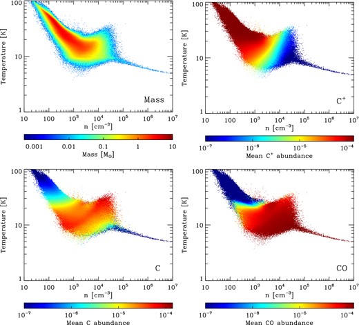
Physical state of the cloud just before the onset of star formation. The top-left panel shows the 2D PDF of gas temperatures and densities within the cloud, weighted by the amount of mass present in each region of density–temperature space. The remaining panels show the same plot of densities and temperatures, but in this case, the shading indicates the mean fractional abundance of C⁺, C or CO present at each point.

Above a number density n ∼ 1000 cm⁻³, the cloud temperature becomes largely independent of the density, although since there is considerable scatter in the temperature in this regime, it is somewhat misleading to describe the gas as isothermal. This scatter is related to the large scatter in the effective extinction seen by different regions of the gas that have similar densities (see Fig. 2), which leads to substantial variations in the efficiency of photoelectric heating, as well as in the chemical state of the gas. One notable feature in this regime is the distinct bump in the temperature distribution at n ∼ 2 × 10⁴ cm⁻³ and T ∼ 20 K, caused by H₂ formation heating (Glover & Clark 2012a).

Figure 2.

Open in new tabDownload slide

As Fig. 1, but for the density and the effective visual extinction, A_{V, eff} (see Section 3.1).

Finally, at n > 10⁵ cm⁻³, the scatter in the gas temperature largely disappears, and the temperature once again begins to decrease with increasing density. This feature corresponds to the point at which the gas and dust temperatures become strongly coupled, owing to efficient thermal energy transfer between the gas and the dust. Above this density, the gas temperature closely tracks the dust temperature. Since the dust temperature is unaffected by velocity gradients within the gas and varies only weakly with A_V owing to the steep temperature dependence of the dust cooling rate (⁠|$\Lambda _{\rm dust} \propto T_{\rm dust}^{6}$|⁠), most of the scatter in the temperature distribution disappears once we enter this regime.

If we now look at the remainder of the panels in Fig. 1, which illustrate the chemical state of the carbon in the gas as a function of temperature and density, we see that as we move to higher densities, we move from a regime dominated by C⁺ to one in which neutral atomic carbon dominates, and then finally to a CO-dominated regime. Neutral atomic carbon is present at a variety of different densities in the range 100 < n < 5 × 10⁴ cm⁻³, but becomes very rare at higher densities, where almost all of the available carbon is locked up in CO.

In addition, it is clear that there is little neutral atomic carbon present in the warmer gas with T > 30 K. This is easy to understand, as temperatures T > 30 K are found only in regions where the extinction is low, so that photoelectric heating is effective, and in these regions, photoionization of C to C⁺ occurs rapidly.

It is also interesting to look at how the chemical state of the gas varies as a function of extinction. However, in this case we need to be careful about how we quantify the extinction. A common choice is to work in terms of the line-of-sight value, which we will denote in this paper simply as A_V. Although this choice is simple, and is the same as the definition that we would use observationally, it is less than ideal when one is considering a turbulent cloud, as there is no guarantee that the extinction in other directions has much to do with the extinction along our particular line of sight. As an extreme example, consider the case where we happen to be looking along the long axis of a filament: we would see a high extinction, even though the extinction in directions perpendicular to the filament may be small.

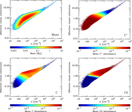
In Fig. 2, we show how the chemical state of the gas varies as a function of density and A_{V, eff}. We see that although density and effective extinction are correlated, there is significant scatter in the relationship, particularly at low densities. This scatter can amount to as much as an order of magnitude variation in A_{V, eff} at a given density, and since photochemical rates typically depend exponentially on A_{V, eff}, the scatter in their values at a given density can be far larger (cf. Glover et al. 2010, who find a similar result for turbulent clouds without self-gravity).

Fig. 2 also shows us that C⁺ dominates in the region with A_{V, eff} < 1, as we would expect given the effectiveness of carbon photoionization at low A_{V, eff}. There is also some neutral atomic carbon in this region, but very little CO. Neutral atomic carbon begins to take over from C⁺ above A_{V, eff} = 1, peaking at A_{V, eff} ∼ 2–3, and then declining at higher extinctions as CO starts to dominate.

We see, therefore, that the behaviour of C⁺, C and CO in our turbulent clouds is very similar to that seen in 1D photodissociation region (PDR) cloud models, which find a similar layering as one moves from low to high extinctions. The main differences here are the much larger scatter that we have in the turbulent case, owing to the scatter in the n–A_{V, eff} relationship, and the fact that the regions with A_{V, eff} ∼ 2–3 where C dominates are not found only at the edges of the cloud, but instead are distributed throughout the cloud.

It is also useful to quantify how much of the total mass of neutral atomic carbon in the cloud is located at each density and temperature. In Fig. 3, we show how the mass of the cloud below a density n varies as we vary n. We see that the majority of the gas is located in the density range 100 < n < 10⁴ cm⁻³, with less than 10 per cent to be found at higher or lower densities. We also show in this figure the same quantity for the neutral atomic carbon, i.e. how much of the total mass of C is located below a density n for a range of different values of n. This follows the line for the total gas mass quite closely, although the fraction of the mass of neutral carbon at n < 1000 cm⁻³ is a little smaller than the fraction of the total mass at these densities, since this lower density material contains significant amounts of C⁺. If we compare the distribution of the neutral carbon with the critical densities for the 1 → 0 and 2 → 1 transitions (illustrated by the vertical lines), we see that roughly 60 per cent of the carbon is located below the critical density for the 1 → 0 transition and roughly 80 per cent is located below the critical density for the 2 → 1 transitions. The values for the critical densities plotted here were computed assuming a gas temperature of 20 K, but in practice have little dependence on the temperature. We can therefore conclude that if the [C i] emission is optically thin, much of it will be subthermal, meaning that analyses that assume local thermodynamic equilibrium (LTE) level populations for the carbon may give misleading results. We will return to this point in Section 3.3.

Figure 3.

Open in new tabDownload slide

Cumulative fraction of the total cloud mass located at or below number density n (solid line), plotted as a function of n. We also show the cumulative atomic carbon mass fraction (dotted line), i.e. the fraction of the total amount of atomic carbon located at or below n, plotted as a function of n. The vertical dashed line indicates the critical density of the [C i] 1 → 0 transition, computed assuming that all of the hydrogen is in molecular form, and that the gas temperature is 20 K. The vertical triple dot dashed line indicates the critical density for the 2 → 1 transition, computed with the same assumptions.

Finally, it is also interesting to perform a similar analysis for the cumulative mass fractions of total gas and neutral atomic carbon as a function of temperature. This is illustrated in Fig. 4. We see that almost half of the total gas mass is located in the temperature range 10 < T < 20 K, and that there is almost no gas with T < 10 K or T > 100 K. We also see that, once again, the result for the neutral carbon closely tracks that for the total gas mass.

Figure 4.

Open in new tabDownload slide

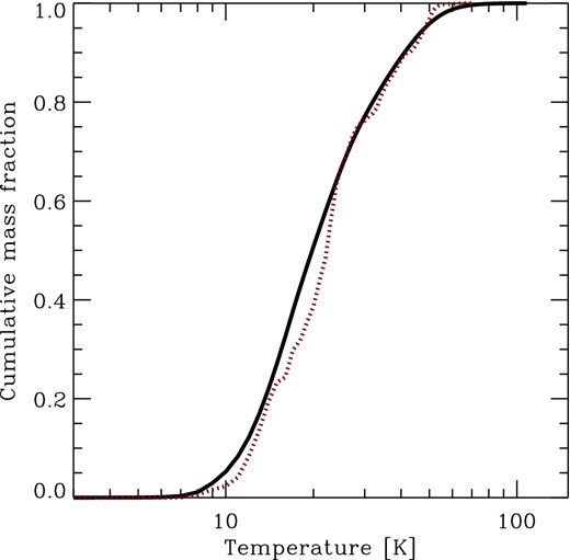
Cumulative fraction of the total cloud mass located at or below gas temperature T (solid line), plotted as a function of T. We also show the cumulative atomic carbon mass fraction (dotted line) as a function of T.

3.2 How much of the cloud is traced by [C i] emission?

We saw in the previous section that the range of densities containing most of the neutral atomic carbon is very similar to the range of densities containing the bulk of the cloud's mass. Moreover, although most of the atomic carbon is found in gas with densities below the critical densities for the 1 → 0 and 2 → 1 transitions, it does not lie very far below n_crit. Therefore, although we expect the emission to be subthermal, it will not be strongly subthermal. Furthermore, the neutral atomic carbon is found primarily in gas with temperatures in the range 10 < T < 50 K, and these temperatures are high enough to excite the 1 → 0 transition relatively easily.

Taken together, these factors suggest that [C i] emission should be a good tracer of the gas in the cloud. To investigate whether this is the case, we have used radmc-3d to make maps of the velocity-integrated intensity of the [C i] 1 → 0 and 2 → 1 lines produced by the cloud. These are shown in Fig. 5, together with the cloud column density and the integrated intensity in the ¹²CO J = 1 → 0 transition. We see that there is a good correlation between the structure that we see in the column density map and in the [C i] 1 → 0 emission map. The [C i] emission traces most of the structure down to a total hydrogen column density of approximately N_H = 10²¹ cm⁻², but does not pick out the low-density gas at the edges of the cloud. Comparing this map with the CO emission map, we see that both tracers pick out the same basic cloud structure, but that [C i] appears to do a slightly better job close to the edges of the cloud. The [C i] 2 → 1 emission also seems to be a good tracer of cloud structure in the denser regions, but becomes extremely faint towards the edges of the cloud.

Figure 5.

Open in new tabDownload slide

Top left: map of the total column density of hydrogen nuclei, N_H. The area shown is approximately 16 pc by 16 pc and contains most of the mass of the cloud. Top right: map of velocity-integrated intensity in the [C i] 1 → 0 transition, computed using radmc-3d with the LVG approximation. Bottom left: the same as in the top-right panel, but for the [C i] 2 → 1 transition. Bottom right: the same as in the top-right panel, but for the J = 1 → 0 transition of ¹²CO.

The widespread [C i] emission that we see in our map is very different from the limb-brightened emission predicted by simple 1D PDR models, but is qualitatively consistent with the predictions of clumpy PDR models and with observations of [C i] in real GMCs, which typically find a good correlation between the [C i] and CO emission (see e.g. Stark & van Dishoeck 1994; Kramer et al. 2008). This is a testament to the central role that turbulence plays in structuring the cloud. As we have already seen, the neutral atomic carbon in our model cloud is found at a similar range of effective visual extinctions to those that we would expect based on PDR model results. The key difference is that gas with this effective extinction is not located in a single coherent structure at the edge of the cloud. Because of the turbulent motions, the cloud is highly structured, allowing radiation to penetrate deep into the interior (see also Bethell et al. 2004; Bethell, Zweibel & Li 2007). The [C i] emitting surfaces that we see are therefore found throughout the cloud and are present along most lines of sight. The crucial role that density substructure within GMCs plays in explaining the observed [C i] emission has been understood for some time (see e.g. Genzel et al. 1988; Stutzki et al. 1988; Plume, Jaffe & Keene 1994; Kramer et al. 2004), and our results strongly support this picture.

Having established that the [C i] 1 → 0 line appears to be a promising gas tracer, the next step is to quantify what fraction of the molecular gas in the cloud it allows us to observe. A simple starting point is to compute what fraction of the total H₂ mass is found along lines of sight with [C i] integrated intensities greater than some minimum value |$W_{{\rm C}\,{\small {i}}, 1-0, {\rm min}}$|⁠, and then to look at how this value changes as we vary |$W_{{\rm C}\,{\small {i}}, 1-0, {\rm min}}$|⁠. The results of this analysis are shown in Fig. 6, together with similar results for the [C i] 2 → 1 line, the ¹²CO J = 1 → 0 line and the ¹³CO J = 1 → 0 line.

Figure 6.

Open in new tabDownload slide

Cumulative fraction of the H₂ mass in the cloud traced by the [C i] 1 → 0 transition (the black solid line) and the 2 → 1 transition (the red solid line), plotted as a function of the minimum integrated intensity in the line. The same quantity is also shown for the ¹²CO J = 1 → 0 transition (upper blue dashed line) and the ¹³CO J = 1 → 0 transition (lower blue dashed line).

We see that for all of the lines, the fraction of the cloud that we detect is a strong function of the minimum integrated intensity. In the case of [C i] 1 → 0, almost 80 per cent of the molecular mass of the cloud is located along lines of sight with integrated intensities in the narrow range |$1 < W_{{\rm C}\,{\small {i}}, 1-0, {\rm min}} < 5\,{\rm K\,km\,s^{-1}}$|⁠. In the case of the [C i] 2 → 1 line, we see similar behaviour, but the minimum integrated intensity required in order to detect any given amount of the molecular gas is typically at least a factor of a few smaller.

If we compare this with the behaviour of ¹²CO, we see that if our minimum integrated intensity for both lines is greater than 0.3 K km s⁻¹, then ¹²CO is a superior tracer of the molecular mass. Only once we start to look along very faint sightlines does the [C i] emission start to trace regions that would be unobserved in ¹²CO. For ¹³CO, the story is rather different. For integrated intensities greater than around 1 K km s⁻¹, the behaviour of the ¹³CO J = 1 → 0 line and the [C i] 1 → 0 line is very similar. At lower integrated intensities, the [C i] line becomes the better tracer, allowing one to study the 15–20 per cent of the molecular mass of the cloud that is not well traced by ¹³CO.

3.3 Determining the [C i] excitation temperature

In Fig. 7, we show the results obtained using these two approaches. In both cases, we restrict the region plotted to the set of sightlines with |$W_{{\rm C}\,{\small {i}}, 1-0} > 0.1\,{\rm K}\,{\rm km\,s^{-1}}$|⁠. By enforcing this restriction, we avoid the poorly resolved regions at the edge of the cloud that are too faint in [C i] to be observable with current instruments. We see from this figure that equation (9) predicts values for T_ex of around 15–20 K, with significantly higher values of up to 40 K along the lines of sight passing through the densest gas. On the other hand, equation (10) predicts values of T_ex that are close to 10 K through much of the cloud, dropping to only a few K at the edges of the cloud.

Figure 7.

Open in new tabDownload slide

Top left: estimate of the mean excitation temperature of the neutral carbon atoms along each line of sight, computed from the ratio of the integrated intensities of the [C i] 2 → 1 and 1 → 0 transitions (equation 9). This estimate assumes that the gas is optically thin in both transitions, and hence yields artificially high values towards optically thick regions. Top right: an alternative estimate of T_ex, computed using equation (10), based on a procedure introduced by Dickman (1978). This estimate assumes that the [C i] 1 → 0 line is optically thick and so underestimates T_ex along optically thin sightlines. Bottom left: mean value of T_ex for the 1 → 0 transition along each sightline, computed as a weighted average of the value in each grid cell, with the number density of atomic carbon atoms used as the weighting function (equation 12). Bottom right: column temperature of the carbon atoms along each line of sight, computed using equation (13).

Comparison of the different maps shows that both of our approximations give biased views of T_ex. Equation (9) predicts excitation temperatures that are systematically too large, particularly for the densest lines of sight. At low column densities, this error comes about because equation (9) is actually a measure of the excitation temperature associated with the 2 → 1 transition. Although this is often assumed to be the same as the excitation temperature associated with the 1 → 0 transition, we find that in practice the two excitation temperatures differ by several K in much of the [C i] emitting gas. Towards dense regions, the performance of equation (9) becomes even worse because of its neglect of the effects of line opacity. If one or both of the [C i] lines becomes optically thick, then the ratio of integrated brightness temperatures for the two transitions is no longer proportional to the ratio of the column densities of the J = 1 and 2 level, and hence equation (9) is no longer valid. If the 2 → 1 transition becomes optically thick while the 1 → 0 transition remains optically thin, then this leads to an underestimate of N₂/N₁ and hence an underestimate of the excitation temperature. In the far more likely case that the 1 → 0 transition becomes optically thick while the 2 → 1 transition remains optically thin (see Appendix B), then we overestimate N₂/N₁ and hence overestimate T_ex, potentially by a large amount.

As one would expect, equation (10) performs much better along the optically thick sightlines, predicting values for T_ex that are within a few per cent of the true ones, providing that we restrict our attention to lines of sight with |$W_{{\rm C}\,{\small {i}}, 1-0} > 3\,{\rm K}\,{\rm km}\,{\rm s^{-1}}$|⁠. However, it systematically underestimates T_ex along lines of sight that have low τ and low |$W_{{\rm C}\,{\small {i}}, 1-0}$|⁠, such as those near the edges of the cloud. In practice, the fact that the real excitation temperature does not vary very strongly over the cloud means that we can construct a reasonably accurate estimate of T_ex by using equation (10) for lines of sight with |$W_{{\rm C}\,{\small {i}}, 1-0} > 3\,{\rm K}\,{\rm km}\,{\rm s^{-1}}$| and adopting a constant value for lines of sight with lower |$W_{{\rm C}\,{\small {i}}, 1-0}$| that is the mean of the value inferred for the bright sightlines.

The resulting column temperature map is shown in panel (d) of Fig. 7. If we compare it with the map of mean excitation temperatures, we see that there is relatively good agreement between T_{col, C} and T_{ex, mean} along lines of sight that pass through the highest density parts of the cloud, but that the values diverge significantly as we move towards the edges of the [C i] map and look along lines of sight probing lower density gas. This behaviour is simple to explain. Along high column density lines of sight, most of the [C i] emission that we see comes from high density gas that lies close to or above the [C i] critical density. The carbon atoms in this gas are in LTE, and hence T_ex ≃ T_kin. Along lower column density lines of sight, the mean kinetic temperature of the gas is higher, since the mean gas density is lower, and the gas is also less well shielded from the external radiation field. However, the lower gas density also means that most of the carbon atoms are in regions with n < n_crit, and hence are subthermally excited, with T_ex < T_kin. (Similar results have recently been reported for ¹²CO J = 1 → 0 line emission by Molina et al., in preparation). In practice, we find that if we average over all lines of sight with detectable [C i] emission, the resulting mean T_ex is around 30 per cent lower than the mean column temperature. We can reduce the discrepancy to ∼10 per cent if we restrict our attention to lines of sight with |$W_{{\rm C}\,{\small {i}}, 1-0} > 4\,{\rm K}\,{\rm km\,s^{-1}}$|⁠, and to ∼5 per cent if we look only at regions with |$W_{{\rm C}\,{\small {i}}, 1-0} > 6\,{\rm K}\,{\rm km\,s^{-1}}$|⁠.

An important lesson that we can draw from these results is that, contrary to what is often assumed, a significant fraction of the neutral atomic carbon in molecular clouds is not in LTE, and is only subthermally excited. We can confirm this interpretation by comparing the PDF of the integrated intensities of the two [C i] transitions that we obtain from our LVG analysis with the corresponding PDFs that we get if we assume LTE level populations throughout the gas (Fig. 8). We see that the LVG approach produces systematically fainter emission than the LTE analysis, consistent with what we expect if a significant proportion of the carbon atoms are subthermally excited.

Figure 8.

Open in new tabDownload slide

PDF of the velocity-integrated emission in the [C i] 1 → 0 (red) and 2 → 1 (blue) transitions. The solid lines give the results of our LVG analysis, while the dashed lines show the distribution of integrated intensities that we get if we assume LTE level populations. The difference between the LVG and LTE results demonstrates that a significant fraction of the carbon atoms are subthermally excited.

3.4 [C i] emission as a probe of column densities

3.4.1 Tracing the total column density

CO emission is often used as a tracer of column densities within molecular clouds. However, its ability to do this is hampered by a couple of significant problems. It has been understood for a long time that at high column densities, ¹²CO emission becomes optically thick, meaning that it is no longer a good tracer of N_CO or of the total column density of the cloud (see e.g. Scoville & Solomon 1974, for an early discussion of this point). On the other hand, at low column densities, W_CO falls off sharply with decreasing A_V owing to the effects of CO photodissociation (Goodman, Pineda & Schnee 2009; Shetty et al. 2011a). This is illustrated in Fig. 9, where we plot the 2D PDF of W_CO versus A_V that we find in our simulation. Although the two quantities are clearly correlated, the correlation is close to linear only over a small range of visual extinctions around A_V ∼ 3. At higher A_V, the correlation becomes sublinear, owing to the effects of the line opacity, while at lower A_V, there is a rapid fall-off in W_CO owing to the loss of CO from the gas due to photodissociation. Moreover, it is also clear that even in the regime where W_CO and A_V have a correlation that is close to linear, there is substantial scatter around this correlation.

Figure 9.

Open in new tabDownload slide

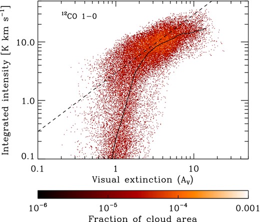
2D PDF of the integrated intensity in the ¹²CO J = 1 → 0 line, W_CO, plotted as a function of the visual extinction. The dashed line indicates a linear relationship between W_CO and A_V and is there to guide the eye. The solid line shows the geometric mean of W_CO as a function of A_V. The points are colour-coded according to the fraction of the total cloud area that they represent.

We can improve on this situation by looking at emission from ¹³CO instead of ¹²CO. The abundance of carbon-13 in the interstellar medium is much smaller than that of carbon-12, and hence the ¹³CO abundance is much smaller than the ¹²CO abundance. Consequently, the optical depths of the ¹³CO rotational transitions are much smaller than for ¹²CO, making ¹³CO a more reliable tracer of the gas column density along high extinction sightlines (Pineda et al. 2008; Goodman et al. 2009). This is illustrated in Fig. 10, where we show the 2D PDF of the integrated intensity in the J = 1 → 0 line of ¹³CO, W_13CO, versus the visual extinction.

Figure 10.

Open in new tabDownload slide

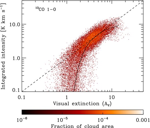
As Fig. 9, but for the J = 1 → 0 transition of ¹³CO. To compute the ¹³CO emission map, we have assumed a constant ratio of 60:1 between ¹²CO and ¹³CO.

Fig. 10 demonstrates that, as expected, ¹³CO is a significantly better tracer of the column density than ¹²CO. The relationship between W_13CO and A_V is extremely close to linear for visual extinctions in the range 3 < A_V < 10, although there are hints that opacity effects are beginning to become important at A_V ∼ 10. However, as in the case of ¹²CO, the relationship breaks down at low A_V owing to the photodissociation of CO.

Since neutral atomic carbon is primarily found at lower gas densities and lower extinctions than CO, we might reasonably expect [C i] emission to be a better tracer of A_V at low extinctions than CO. To test this, we plot in Fig. 11 the 2D PDF of the integrated intensity of the [C i] 1 → 0 line. We see that there is a good linear correlation between |$W_{{\rm C}\,{\small {i}}, 1-0}$| and A_V for visual extinctions in the range 1.5 < A_V < 7. At higher extinctions, the correlation becomes sublinear, possibly because an increasing fraction of this high extinction gas consists of CO rather than C, while at A_V < 1.5, the correlation breaks down owing to the photoionization of C. Comparing our results for C and ¹³CO, we see that neutral atomic carbon is a better tracer of low column density material, while ¹³CO is to be preferred at high column densities. We also note that although the difference between A_V = 1.5 and 3 may seem minor, it actually corresponds to approximately 20 per cent of the total mass of the cloud, consistent with our results in Section 3.2.

Figure 11.

Open in new tabDownload slide

As Fig. 9, but for the [C i] 1 → 0 line.

We have also examined how well the [C i] 2 → 1 line traces the total column density (Fig. 12). As with the lower energy transition, we see that there is a good linear correlation between the integrated intensity of the line and the visual extinction over a wide range of A_V. At low A_V, the correlation breaks down at A_V ∼ 2, a slightly higher value than for the 1 → 0 line, but at high A_V the 2 → 1 line performs better than the 1 → 0 line, with the correlation between |$W_{{\rm C}\,{\small {i}}, 2-1}$| and A_V remaining approximately linear up to the highest extinctions probed in our study.

Figure 12.

Open in new tabDownload slide

As Fig. 9, but for the [C i] 2 → 1 line. Note the change in the range of values displayed on the y-axis.

However, it is important to note that even at the highest A_V examined here, the 2 → 1 line has a much lower integrated intensity than the 1 → 0 line. This fact, plus the greater atmospheric opacity at the frequency of the 2 → 1 line compared to the 1 → 0 line means that in practice, the small improvement that one gets by observing the 2 → 1 line is unlikely to justify the additional observing time required to map it to the same level of sensitivity. Whether this is true for all GMCs or merely those with properties similar to those of the cloud modelled here is an interesting question, but is beyond the scope of the present study.

Finally, we note that our finding here that [C i] emission is a relatively good tracer of the column density over a significant range of A_V was already anticipated to some extent observationally. For example, in their study of NGC 891, Gerin & Phillips (2000) found a good spatial correlation between [C i] 1 → 0 emission and 1.3 mm dust continuum emission, which they interpreted as evidence that [C i] emission is a good tracer of the gas column density.

3.4.2 Tracing the H₂ column density

In the previous section, we saw that one of the main drawbacks with using [C i] to trace the structure of the cloud is that it becomes very faint along low A_V lines of sight, and hence misses material at the edges of the cloud. However, this low density, low extinction gas will largely be composed of H i, rather than H₂, and so it is worthwhile to examine whether there is a better correlation between the [C i] integrated intensity and the H₂ column density than there is between the [C i] integrated intensity and the total column density.

In Fig. 13, we show a 2D PDF of |$W_{{\rm C}\,{\small {i}}, 1-0}$| as a function of the H₂ column density, |$N_{\rm H_{2}}$|⁠. The behaviour we see in this plot is qualitatively similar to the behaviour of the |$W_{{\rm C}\,{\small {i}}, 1-0}$|–A_V relationship. [C i] emission traces H₂ well at intermediate H₂ column densities, |$5 \times 10^{20} < N_{\rm H_{2}} < 10^{22}\,{\rm cm^{-2}}$|⁠, but underestimates the molecular gas column density at high column densities, owing to the optical depth of the [C i] line. The correlation between [C i] emission and H₂ column density also breaks down at low column densities, but it is clear from comparing Figs 11 and 13 that [C i] is a better tracer of the H₂ column density than of the total column density in this regime.

Figure 13.

Open in new tabDownload slide

2D PDF of the integrated intensity in the [C i] 1 → 0 line, plotted as a function of the H₂ column density, |$N_{\rm H_{2}}$|⁠. The dashed line indicates a linear relationship between |$W_{{\rm C}\,{\small {i}}, 1-0}$| and |$N_{\rm H_{2}}$| and is there to guide the eye. The solid line shows the geometric mean of |$W_{{\rm C}\,{\small {i}}, 1-0}$| as a function of |$N_{\rm H_{2}}$|⁠. The points are colour-coded according to the fraction of the total cloud area that they represent.

Offner et al. (2014) also computed the mean value of |$X_{\rm C\,{\small {i}}}$| for each of their simulations. For their run with G₀ = 1.0, which is probably the closest analogue to our simulated cloud, they obtained a value |$X_{\rm C\,{\small {i}}} = 1.1 \times 10^{21}\,{\rm cm^{-2}\,K^{-1}\,km^{-1}\,s}$|⁠. For comparison, we find a value |$X_{\rm C\,{\small {i}}} = 1.01 \times 10^{21}\,{\rm cm^{-2}\,K^{-1}\,km^{-1}\,s}$|⁠, within 10 per cent of their result.

3.4.3 Measuring the column density of C

In Section 3.4.1, we saw that [C i] emission is a good tracer of the total column density of the cloud over a wide range of visual extinctions. However, the relationship we derived between |$W_{{\rm C}\,{\small {i}}, 1-0}$| and A_V (equation 14) was completely empirical, and hence we cannot be confident that the same relationship will hold for other molecular clouds, whether simulated or real. Ideally, what we would like to be able to do is to infer the column density of neutral atomic carbon, N_C, from our observations and then to infer A_V from N_C. However, this is not straightforward, as we demonstrate below.

Although we have seen already that the [C i] 1 → 0 line does not remain optically thin over the entire range of column densities probed in our model cloud, it is nevertheless interesting to examine how well we can recover N_C in the case where we ignore any optical depth effects, and how large an error we make in the total neutral atomic carbon abundance we derive for the cloud when using this simplified approach.

In Fig. 14(a), we show a 2D PDF of the estimate of N_C that we derive if we assume optically thin [C i] emission (N_{C, est}) versus the true value of N_C measured from the simulation. As before, we show values only for those lines of sight with |$W_{{\rm C}\,{\small {i}}, 1-0} > 0.1\,\,{\rm K\,km\,s^{-1}}$|⁠. To compute our column density estimate, we need to know the mean excitation temperature along each line of sight. For this first estimate, we set T_ex = T_{ex, mean}, the weighted mean excitation temperature given by equation (12) for each line of sight. We see from the figure that for atomic carbon column densities of less than a few times 10¹⁶ cm⁻², there is very good agreement between N_{C, est} and N_C. At higher column densities, however, N_{C, est} falls below N_C; i.e. it becomes an underestimate. This is easy to understand as a consequence of the growing optical depth of the [C i] lines with increasing N_C, an effect which is not accounted for in our simple estimate.

Figure 14.

Open in new tabDownload slide

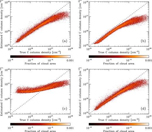
(a) 2D PDF showing the estimated column density of neutral atomic carbon as a function of the true column density. The estimated column density was computed using the procedure described in Section 3.4.3, with the excitation temperature for each line of sight taken to be a weighted mean of the actual excitation temperature. At carbon column densities greater than a few times 10¹⁶ cm⁻², we underestimate N_C because we do not account for the effects of line opacity. As in Figs 9–11, the colour-coding corresponds to the fraction of the total area of the cloud represented by each point. (b) As panel (a), but using the estimate of T_ex given by equation (9). We see that because equation (9) overestimates the excitation temperature associated with the 1 → 0 transition, our derived values of N_C systematically underestimate the true values. (c) As panel (a), but using the estimate of T_ex given by equation (10). This estimate performs very badly: at low column densities, we underestimate T_ex and hence overestimate N_C, while at high column densities, our values for T_ex are much more accurate but the neglect of optical depth effects means that we now underestimate N_C. (d) As panel (a), but using the estimate of T_ex given by equation (10) for lines of sight with |$W_{{\rm C}\,{\small {i}}, 1-0} > 3\,{\rm K}\,{\rm km}\,{\rm s^{-1}}$| and adopting a constant value for the fainter lines of sight that is equal to the mean of the values determined for the bright sightlines.

In practice, T_{ex, mean} is not an observable quantity. Therefore, in the other panels of Fig. 14 we explore what happens if we use the different estimates of T_ex that we derived in Section 3.3 to compute our estimate of N_C. In Fig. 14(b), we show the result that we obtain when we set T_ex = T_{ex, est}, the excitation temperature estimate given by equation (9). We see that although there is still a good correlation between N_C and N_{C, est} at low column densities, our column density estimate is systematically offset from the true value by a factor of approximately 0.7. This behaviour is consistent with our earlier finding that T_{ex, est} is an overestimate of the true excitation temperature, as this means that our derived value for N₀ is too small.

In Fig. 14(c), we show what happens if we use T_{ex, est, 2}, the estimate of T_ex that we obtained from the optically thick analysis. We see that in this case, there is very poor agreement between N_{C, est} and N_C. This is not unexpected, as in this approach we assume mutually contradictory things for the [C i] emission. Our derivation of the excitation temperature assumes that [C i] is optically thick, but our expression for N_C assumes that the emission is optically thin. Along sightlines where the emission is actually optically thin, we derive excitation temperatures that are too small and hence predict values for the column density of carbon atoms in the J = 0 level that are much higher than the true value, leading to values of N_{C, est} that are also far too large. On the other hand, along sightlines where the emission is actually optically thick, our estimated values of T_ex are far more reasonable, but our expression for N_C is no longer accurate, because it does not account for the effects of line opacity. In this regime, we therefore underestimate N_C.

Finally, in Fig. 14(d), we show the results we obtain if we compute T_ex for lines of sight with |$W_{{\rm C}\,{\small {i}}, 1-0} > 3\,{\rm K}\,{\rm km}\,{\rm s^{-1}}$| using equation (10), and adopt a constant value for the fainter lines of sight that is equal to the mean of the values determined for the |$W_{{\rm C}\,{\small {i}}, 1-0} > 3\,{\rm K}\,{\rm km}\,{\rm s^{-1}}$| sightlines. We see that this strategy performs well at low N_C: estimates for N_C along individual sightlines can differ from the true values by as much as 50 per cent, but there is no systematic bias towards low or high values. At high N_C, optical depth effects once again cause this method to break down.

Figure 15.

Open in new tabDownload slide

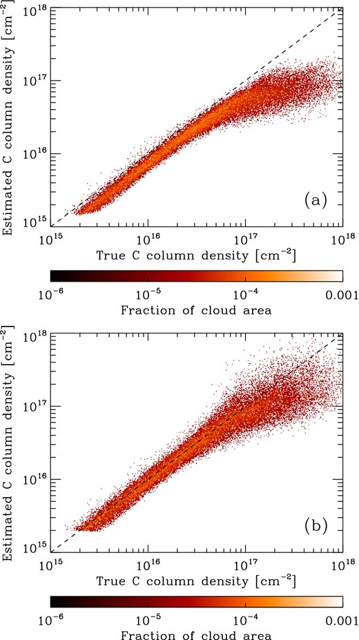
(a) 2D PDF showing the estimated column density of neutral atomic carbon as a function of the true column density, computed using the estimate of T_ex given by equation (9) and corrected for opacity using equations (17) and (19). As in the previous figures, the colour-coding corresponds to the fraction of the total area of the cloud represented by each point. (b) As (a), but using an estimate of T_ex derived from the ¹²CO peak brightness temperature, as described in more detail in the text.

The results that we obtain with this approach are plotted in Fig. 15. We see that the column density estimates yielded by this technique agree well with the true values for column densities up to N_C ∼ 7 × 10¹⁶ cm⁻². At higher column densities, this technique does not completely correct for the effects of the opacity, and so we still underestimate the true column density along most sightlines in this regime. Nevertheless, even here we see significant improvement in comparison to the uncorrected case, albeit at the cost of substantially increased scatter.

We have also examined how much of the atomic carbon in the cloud we fail to detect owing to the line opacity, and how good our various approximations are at recovering this missing material. The total atomic carbon content that we infer if we use the actual column-averaged excitation temperatures but do not correct for opacity is approximately 47 per cent of the true value, i.e. we miss around half of the atomic carbon. Using excitation temperatures derived from the [C i] line ratio and correcting for opacity actually makes the situation worse: the small improvement at high N_C is swamped by the effects of the systematic underestimate at low N_C, and we recover only 37 per cent of the total atomic carbon. Finally, using values for T_ex estimated from the ¹²CO emission does improve matters, but even in this case we recover only 65 per cent of the total atomic carbon. An important conclusion that we can draw from this result is that estimates in the literature of the atomic carbon content of real molecular clouds that are based on observations of the [C i] emission will typically be too small, possibly by as much as a factor of 2.

Given an estimate of N_C, a further problem that we face is how to convert from this to the total column density. Along a given line of sight, N_C and N_{H, tot}, the total hydrogen column density, are related by |$N_{\rm H, tot} = N_{\rm C} \bar{x}_{\rm C, los}^{-1}$|⁠, where |$\bar{x}_{\rm C, los}$| is the fractional abundance of atomic carbon weighted by mass and averaged along the line of sight. The mass-weighted average for the cloud as a whole is given by |$\bar{x}_{\rm C} = 1.60 \times 10^{-5}$|⁠, but as we have already seen, the local abundance is not constant, but instead varies as a function of density and position in the cloud.

In Fig. 16, we show how |$\bar{x}_{\rm C, los}$| varies as a function of the visual extinction. We see that there is a systematic increase in the mean abundance as we move to higher extinctions. This is particularly pronounced around A_V ∼ 1, where we first start to probe regions that are well shielded from the ISRF, but even at much higher A_V we still see an increase. Using the mean value for the whole cloud as a proxy for |$\bar{x}_{\rm C, los}$| is a reasonable approximation only for visual extinctions ∼ a few, but would lead one to significantly underestimate the total column density along diffuse lines of sight and overestimate it along dense sightlines. Moreover, |$\bar{x}_{\rm C}$| is not an observable quantity (unless the total column density of the cloud is already known), but must instead be estimated using a chemical model of the cloud, such as that included in our hydrodynamical simulation. This introduces yet more uncertainty into the final column density estimate, and leading us to conclude that this technique for estimating N_{H, tot} is likely in practice to be much less accurate than simply using the correlation between |$W_{{\rm C}\,{\small {i}}, 1-0}$| and A_V discussed in the previous section.

Figure 16.

Open in new tabDownload slide

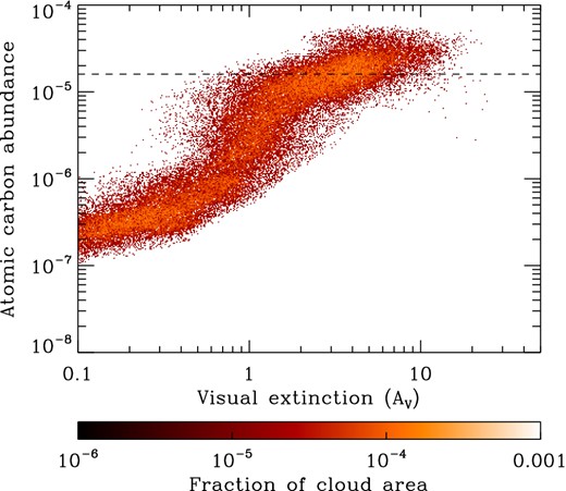
2D PDF showing the line-of-sight averaged fractional abundance of neutral atomic carbon as a function of the visual extinction. The colour-coding corresponds to the fraction of the total area of the cloud represented by each point. The horizontal dashed line indicates the mean fractional abundance in the cloud as a whole.

3.5 Comparison of [C i] and ¹³CO emission

We have seen in the previous subsections that there are some interesting similarities between [C i] 1 → 0 emission and ¹³CO J = 1 → 0 emission. Both tracers are optically thin for a broad range of visual extinctions, and both trace a very similar fraction of the cloud mass when we restrict our attention to regions where the integrated intensity exceeds a few K km s⁻¹. It is therefore worthwhile to directly compare these two tracers in more detail, so that we can better understand their strengths and weaknesses.

In Fig. 17, we examine how the integrated intensity ratio |$R \equiv W_{{\rm C}\,{\small {i}}, 1-0} / W_{\rm 13CO}$| varies over the cloud. In the left-hand panel, we compute this ratio only for lines of sight for which both |$W_{{\rm C}\,{\small {i}}, 1-0}$| and W_13CO exceed 0.1 K km s⁻¹. We see that within this region, R is surprisingly uniform with a value close to 1. This behaviour is in good agreement with observations of the [C i]-to-¹³CO intensity ratio in real clouds (see e.g. Ikeda et al. 2002) that often show almost uniform ratios. It is also clear that R starts to increase towards the edge of the cloud, but the restriction of the image to regions with ¹³CO emission above our 0.1 K km s⁻¹ threshold acts to obscure how large R can grow as we move towards the edge of the cloud. Therefore, in the right-hand panel of Fig. 17, we show how R behaves when we remove this restriction. The colour scale is chosen to emphasize the change in R at the edge of the cloud, although for practical reasons we limit the maximum displayed value to R = 50. Comparing the two maps allows one to see very clearly the envelope of gas around the CO-bright portion of the cloud that is well traced by [C i] but not by ¹³CO.

Figure 17.

Open in new tabDownload slide

Ratio of the integrated intensities of the [C i] 1 → 0 transition and the ¹³CO J = 1 → 0 transition. In the left-hand panel, we show the values only for those lines of sight with W_13CO ≥ 0.1 K km s⁻¹, which serves to emphasize the near uniformity of the intensity ratio within the CO-bright region. In the right-hand panel, we show how the intensity ratio behaves when we remove this restriction. In this case, we have chosen a different colour scale that allows us to highlight the region at the edges of the cloud where there is still bright [C i] emission but no significant ¹³CO emission, resulting in a large value for the intensity ratio. Note that for practical reasons, we limit the maximum displayed value of the ratio to 50.

Figure 18.

Open in new tabDownload slide

Left: reconstruction of the column density distribution, based on the empirical relationship between |$W_{{\rm C}\,{\small {i}}, 1-0}$| and A_V quantified by equation (14). Right: as in the left-hand panel, but this time using the empirical relationship between W_13CO and A_V given by equation (22).

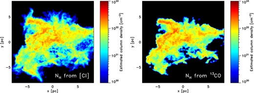
Comparing these two reconstructed maps with the true column density map shown in Fig. 5(a), we see that, as expected, [C i] allows us to better reconstruct the column density distribution towards the edges of the cloud, although we still miss some of the lowest column density material. On the other hand, ¹³CO seems to do better at tracing the highest density peaks, some of which are hard to pick out from the background when using [C i].

Finally, we have also examined how well [C i] and ¹³CO trace the cloud velocity. We have computed cloud-averaged spectra for the [C i] 1 → 0 line and for the ¹³CO J = 1 → 0 line, and have plotted these in Fig. 19, along with a cloud-averaged spectrum for the ¹²CO J = 1 → 0 transition. We see that the line width and strength of the [C i] and ¹³CO are remarkably similar. This is unsurprising, since in both cases, the cloud-averaged spectra are dominated by the bright emission coming from the high-density regions of the cloud, and hence are largely tracing the same material. The fact that the [C i] emission does a better job of tracing the boundaries of the cloud does not greatly affect the average line width, as little of the total [C i] emission is generated in these regions. Finally, the much higher optical depth of the ¹²CO emission means that a larger fraction of the cloud contributes to the cloud-averaged spectrum, resulting in a much brighter line with a greater line width.

Figure 19.

Open in new tabDownload slide

Comparison of the mean brightness temperatures of ¹²CO J = 1 → 0 (solid line), ¹³CO J = 1 → 0 (dotted line) and the [C i] 1 → 0 transition (dashed line), averaged over the entire synthetic image.

4 CONCLUSIONS

In this paper, we have examined in detail the distribution of neutral atomic carbon within a model of a turbulent molecular cloud illuminated by the standard local ISRF, and have also studied the [C i] fine structure emission produced by these carbon atoms. We show that the density substructure created by the turbulence naturally leads to widespread, spatially extended [C i] emission, in good agreement with observations of real molecular clouds.

Most of the neutral carbon in our model is located in gas with a density in the range 100 < n < 10⁴ cm⁻³, and with an effective (angle-averaged) visual extinction A_{V, eff} > 1. This gas is relatively cold – around 80 per cent of the neutral carbon is found in regions with T < 30 K – and so [C i], like CO, is primarily a tracer of the cold, dense phase within molecular clouds, and not the warm, space-filling phase traced by [C ii].

Our results suggest that [C i] 1 → 0 emission is a promising tracer of low column density gas in molecular clouds. Although it is easier to detect the molecular gas using ¹²CO emission than using [C i] emission, the relationship between ¹²CO integrated intensity and the column density of the gas is highly non-linear, owing to the effects of CO photodissociation at low A_V and line opacity at high A_V. One can avoid the worst of the opacity effects by using ¹³CO in place of ¹²CO, but the effects of photodissociation are not so easily overcome. We find that ¹³CO emission is a roughly linear tracer of column density for line-of-sight visual extinctions in the range 3 < A_V < 10, although we caution that the fact that we are neglecting CO freeze-out on to dust grains may affect our results at high A_V. In comparison, the integrated intensity of the [C i] 1 → 0 line is a linear tracer of column density for visual extinctions in the range 1.5 < A_V < 7. Observing [C i] in place of ¹³CO therefore allows one to better study the gas with visual extinctions 1.5 < A_V < 3, which in practice accounts for around 20 per cent of the total mass of the cloud. However, at A_V > 3, ¹³CO is as good a tracer of the cloud as [C i], while also being significantly easier to observe. Our results are consistent with previous work that has suggested that [C i] emission is a good tracer of molecular gas (see e.g. Gerin & Phillips 2000; Papadopoulos, Thi & Viti 2004), although whether this is still true for clouds in other environments (e.g. lower metallicities, higher radiation fields) remains to be seen.

We have studied several different ways of estimating the excitation temperature of [C i] based on the observed emission. We find that the best results are obtained if we use the Dickman (1978) method for computing T_ex along sightlines with integrated intensities |$W_{{\rm C}\,{\small {i}}, 1-0} > 3\,{\rm K}\,{\rm km}\,{\rm s^{-1}}$| and adopt a constant value of T_ex for the fainter sightlines, derived by averaging the estimated values for the bright sightlines. The resulting excitation temperatures are typically T_ex ∼ 11–13 K, and are generally smaller than the kinetic temperature of the emitting gas, indicating that most of the carbon atoms are not in LTE.

Using our estimate for T_ex, we can determine the column density of neutral atomic carbon, N_C, with reasonable accuracy in the regime where N_C is less than a few times 10¹⁶ cm⁻². Comparison of the true and estimated column densities shows that although the error along any particular line of sight may be as high as a factor of 2, there is no systematic offset between the estimated and real values. At higher carbon column densities, however, our estimate becomes inaccurate because it neglects the effects of line opacity, and we start to significantly underestimate the true value of N_C. We find that in practice, we typically miss about half of the total atomic carbon when using this procedure. We have also explored whether using the ¹²CO excitation temperature as a proxy for the [C i] excitation temperature can allow us to better reconstruct N_C in the optically thick regime. We find that it does allow us to partially correct for the effects of opacity, although we still miss as much as a third of the total atomic carbon. We therefore recommend that if one wants to estimate N_C based on observations of the [C i] fine structure lines, then the following procedure should be adopted.

• Determine the excitation temperature of the 1 → 0 line of ¹²CO using equation (21).

• Using this excitation temperature as a proxy for that of [C i], estimate the optical depth in the [C i] 1 → 0 transition using equation (19).

• Compute the column density of atomic carbon in the J = 1 level, N₁, using equations (17) and (18).

• Repeat steps 2 and 3 for the J = 2 level, using the integrated intensity of the 2 → 1 transition in place of that of the 1 → 0 transition, and using E₂₁, ν₂₁ and A₂₁ in place of E₁₀, ν₁₀ and A₁₀.

• Use the excitation temperature estimate together with equation (16) to compute the column density of carbon in the J = 0 level.

• Sum the column densities of the three levels to obtain the final estimate for N_C.

If, as is often the case, the atomic carbon column density is estimated without correcting for opacity effects and with the assumption that the levels have LTE populations, then our study suggests that the resulting values could be in error by as much as a factor of 2.

A major limitation of our present study is the fact that we have restricted our attention to a single example of a turbulent cloud. In future work, we plan to examine a wider sample of clouds, and to explore whether [C i] emission remains a good tracer of the H₂ column density as we reduce the metallicity of the cloud and/or increase the strength of the ambient ISRF. It will also be interesting to explore how the ability of [C i] emission to trace H₂ changes over time as the cloud evolves, as we have seen in previous studies that the CO emission from clouds that are in the process of forming can change quickly on a relatively short time-scale.

The authors would like to thank H. Beuther, F. Bigiel, T. Bisbas, D. Cormier, I. De Looze, S. Madden, S. Malhotra, R. Plume and K. Sandstrom for useful conversations on the topic of this work. They would also like to thank S. Ragan for helpful comments on an earlier draft of this manuscript. Special thanks also go to V. Ossenkopf for stressing to us the potential importance of neutral atomic carbon as a cloud tracer, to J. Carpenter for suggesting that we produce a figure along the lines of what is now Fig. 6, and to the referee, P. Goldsmith, whose detailed and thoughtful referee report allowed us to greatly improve the paper. SCOG, FM and PCC acknowledge support from the DFG via SFB project 881 ‘The Milky Way System’ (subprojects B1, B2, B3, B5 and B8). FM and MM also acknowledge financial support by the International Max Planck Research School for Astronomy and Cosmic Physics at the University of Heidelberg (IMPRS-HD) and the Heidelberg Graduate School of Fundamental Physics (HGSFP). The HGSFP is funded by the Excellence Initiative of the German Research Foundation DFG GSC 129/1. PCC further acknowledges support from the DFG priority programme SPP 1573 ‘Physics of the ISM’ (grant CL 463/2-1). MM also acknowledges support from the Ministry of Education, Science and Technological Development of the Republic of Serbia through the project no. 176021, ‘Visible and Invisible Matter in Nearby Galaxies: Theory and Observations’ and support provided by the European Commission through FP7 project BELISSIMA (BELgrade Initiative for Space Science, Instrumentation and Modelling in Astrophysics, call FP7-REGPOT-2010-5, contract no. 256772). The simulations described in this paper were performed on the kolob cluster at the University of Heidelberg, which is funded in part by the DFG via Emmy-Noether grant BA 3706, and via a Frontier grant of Heidelberg University, sponsored by the German Excellence Initiative as well as the Baden-Württemberg Foundation.

REFERENCES

APPENDIX A: RESOLUTION STUDY

Any numerical study of the physics of molecular clouds inevitably has to grapple with the issue of limited numerical resolution. Computational limitations prevent us from running our models at arbitrarily high resolution, and so it is important to establish whether this limitation significantly affects the conclusions that we draw from our model clouds. In the present study, there are three potential sources of resolution dependence: the numerical resolution of the hydrodynamical model itself, the size of the Cartesian grid used during our radiative transfer post-processing step, and the discretization of column densities in the column density maps generated by our treecol algorithm. We examine each of these in more detail below.

A1 Hydrodynamical resolution

The simulation that we have studied in detail here was performed using two million SPH particles to simulate 10⁴ M_⊙ of gas. This gives a particle mass of 5 × 10⁻³ M_⊙, which corresponds to a mass resolution of 0.5 M_⊙, if we use the standard convention that any ‘resolved’ structure must consist of at least 100 SPH particles. We have previously shown that this resolution is sufficient to model the star formation rate within our turbulent cloud (Glover & Clark 2012a), but that the low-mass end of the stellar initial mass function is not properly resolved. This suggests that the resolution is sufficient to model the formation of pre-stellar cores, but not sufficient to properly follow the fragmentation that occurs within them. As most of the [C i] emission in our model comes from gas that is at lower densities than the density of a typical pre-stellar core, it is reasonable to assume that two million particles will give us sufficient resolution to accurately model this emission.

To verify this assumption, we have run a higher resolution simulation of the same cloud using 20 million SPH particles. The higher computational cost of this simulation makes it impractical to run it for as long as our lower resolution simulation, and so we have compared the results from the two simulations at a time t = 0.72 Myr, corresponding to roughly 30 per cent of a free-fall time. Turbulence has already created significant density substructure by this point in the evolution of the cloud and substantial amounts of neutral atomic carbon are present.

In Fig. A1, we compare the PDF of |$W_{{\rm C}\,{\small {i}}, 1-0}$| that we obtain in the two different simulations. The only real difference that is apparent is that the high-resolution simulation produces slightly more emission at high values of |$W_{{\rm C}\,{\small {i}}, 1-0}$| than the low-resolution simulation. This may be a result of the fact that in the high-resolution simulation, we are better able to resolve the wings of the density PDF, and hence are capturing slightly more of the emission from dense, [C i] bright gas. However, the effect is small, and the mean [C i] integrated intensity changes by no more than around 5 per cent. It is therefore safe to conclude that the results presented in this study are not sensitive to the limited hydrodynamical resolution of our simulation.

Figure A1.

Open in new tabDownload slide

PDF of the velocity-integrated emission in the [C i] 1 → 0 line, computed at a time t = 0.72 Myr after the beginning of the simulation. The solid line is for a run with two million SPH particles, while the dot–dashed line is for a higher resolution run with 20 million SPH particles. There is slightly more emission from regions with very high integrated intensities in the high-resolution run, but otherwise the two PDFs are very similar.

A2 radmc-3d Post-processing

A second possible source of resolution dependence comes from our post-processing procedure. As described in Section 2.2, radmc-3d cannot presently deal directly with SPH data, and hence we must interpolate our data on to a Cartesian grid before running the code. The results presented in Section 3 are all based on maps produced using a cubical grid with a side length of 5 × 10¹⁹ cm and a grid resolution of 256³ zones. We have examined the sensitivity of our results to the choice of grid resolution by performing a similar post-processing step using a resolution of only 128³ grid zones. In Fig. A2, we compare the PDF of |$W_{{\rm C}\,{\small {i}}, 1-0}$| that we obtain with the two different grid resolutions. We see that they are almost identical, suggesting that our results are insensitive to our choice of grid resolution. In fact, it is easy to understand why this is the case. The size of a zone in the 256³ case is around 0.06 pc. We can estimate the density at which our SPH smoothing length becomes smaller than a single grid zone by writing it as ρ = N_neighM_part/V, where N_neigh is the number of neighbouring SPH particles smoothed over, M_part is the particle mass and V = 4πh³/3, where h is the SPH smoothing length. In our calculations, N_neigh = 50, M_part = 5 × 10⁻³ M_⊙, and hence ρ ≃ 4 × 10⁻²⁴(h/1 pc)⁻³ g cm⁻³. If we now set h = 0.06 pc, we find that ρ ≃ 2 × 10⁻²⁰ g cm⁻³, corresponding to a number density n ≃ 8000 cm⁻³. This value is significantly higher than the [C i] critical density, and Fig. 3 demonstrates that not only is most of the gas in our simulation found at densities below this, but so is most of the neutral atomic carbon. Therefore, the dense regions that are not well resolved by our 256³ grid contribute only a small fraction of the total [C i] emission, and our failure to resolve these regions has little impact on our results.

Figure A2.

Open in new tabDownload slide

PDF of the velocity-integrated emission in the [C i] 1 → 0 line. The two sets of results shown here were produced using different grid resolutions during the radmc-3d post-processing step. The solid line corresponds to a grid resolution of 256³ zones, while the dot–dashed line corresponds to a grid resolution of only 128³ zones. The PDF produced using the lower resolution grid is somewhat noisier, particularly in the tail of the distribution at low intensities, but other than this, there is not a significant difference between the two distributions.

We have also performed a similar analysis for our CO emission maps (see Fig. A3). Once again, we find that our failure to resolve the highest density structures with our Cartesian grid has little impact on our results.

Figure A3.

Open in new tabDownload slide

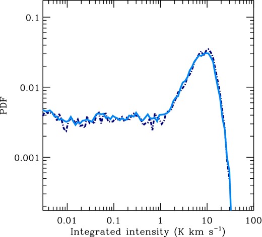
As Fig. A2, but for the ¹²CO J = 1 → 0 line. Once again, we see that our grid resolution is sufficient to capture the bulk of the emission.

A3 TREECOL

The final area in which the effects of limited numerical resolution may make themselves felt is in our treatment of the attenuation of the ISRF within the cloud. We model this using the treecol algorithm (Clark et al. 2012a). This algorithm provides us with an approximate 4π steradian map of the column densities of hydrogen nuclei, H₂ and CO seen by each SPH particle, discretized into a number of equal-area pixels using the healpix pixelation scheme (Górski et al. 2005). The healpix scheme involves splitting up the sphere into 12 equal-area base pixels, each of which can then be further subdivided. The amount of subdivision can be quantified by N_side, the number of pixels along each side of one of the base pixels; the total number of pixels then follows as |$N_{\rm pix} = 12 N_{\rm side}^{2}$|⁠. In treecol, by default we subdivide each of the healpix base pixels into four subpixels, and hence N_side = 2 and N_pix = 48. We have found in testing that this choice appears to give us the best balance between computational efficiency (which argues for a small value for N_pix) and accuracy (which argues for a larger value). However, we have also investigated the extent to which our results depend upon this choice. In Fig. A4, we compare the PDF of integrated intensity in the 1 → 0 line of [C i] that we obtain from our default run with the corresponding distribution produced by a run with N_side = 4 and N_pix = 192. We see that the results are essentially indistinguishable, justifying our decision to use a small value for N_pix.

Figure A4.

Open in new tabDownload slide

PDF of the velocity-integrated emission in the [C i] 1 → 0 line. The solid blue line shows results from a simulation performed using N_pix = 48 healpix pixels in the treecol algorithm, while the dark blue dash-dotted line shows results from a simulation performed using N_pix = 192 healpix pixels. We see that the results are essentially indistinguishable.

APPENDIX B: RELATIVE OPTICAL DEPTHS OF THE [C i] LINES

In this appendix, we examine whether there are any physical conditions in which the 2 → 1 transition of [C i] is optically thick while the 1 → 0 transition remains optically thin.

If we assume that all three fine structure levels of the carbon atom have their LTE level populations, then using this expression, it is easy to show that τ₂₁/τ₁₀ < 1 for all temperatures T < 40 K, and that in the limit of large temperatures, τ₂₁/τ₁₀ ∼ 2. If the level populations are instead significantly subthermal, then the optical depth ratio is much smaller. We therefore see that it is indeed possible for the 2 → 1 transition of [C i] to be optically thick while the 1 → 0 transition remains optically thin, but that it requires rather unusual conditions: the gas must be hot, sufficiently dense that the level populations are close to LTE, and must have a total column density of carbon such that 0.5 < τ₁₀ < 1.0. The last condition is particularly restrictive, as it implies that for any given combination of temperature and density, the range of carbon column densities that gives rise to a situation with τ₁₀ < 1 and τ₂₁ > 1 spans only a factor of 2. For comparison, in our simulations, we find values of N_C spanning almost three orders of magnitude. Therefore, in most cases, either both lines will be optically thin, both will be optically thick, or the 1 → 0 transition will be optically thick while the 2 → 1 transition remains optically thin, with the last possibility being particularly likely when the excitation of the fine structure levels is subthermal.

In the particular case of the cloud modelled in this paper, we can be confident that we are never in a situation with τ₁₀ < 1 and τ₂₁ > 1. As Fig. 1 demonstrates, almost all of the atomic carbon is found in gas with T < 40 K, and the little that is not is found at densities n ≪ n_crit, and hence will be subthermally excited.