The cross-correlation of Mg ii absorption and galaxies in BOSS

Pérez-Ràfols, Ignasi; Miralda-Escudé, Jordi; Lundgren, Britt; Ge, Jian; Petitjean, Patrick; Schneider, Donald P.; York, Donald G.; Weaver, Benjamin A.

doi:10.1093/mnras/stu2645

Abstract

We present a measurement of the cross-correlation of Mg ii absorption and massive galaxies, using the Data Release (DR)11 main galaxy sample of the Baryon Oscillation Spectroscopic Survey (BOSS) of Sloan Digital Sky Survey III (SDSS-III; CMASS galaxies), and the DR7 quasar spectra of SDSS-II. The cross-correlation is measured by stacking quasar absorption spectra shifted to the redshift of galaxies that are within a certain impact parameter bin of the quasar, after dividing by a quasar continuum model. This results in an average Mg ii equivalent width as a function of impact parameter from a galaxy, ranging from 50 kpc to more than 10 Mpc in proper units, which includes all Mg ii absorbers. We show that special care needs to be taken to use an unbiased quasar continuum estimator, to avoid systematic errors in the measurement of the mean stacked Mg ii equivalent width. The measured cross-correlation follows the expected shape of the galaxy correlation function, although measurement errors are large. We use the cross-correlation amplitude to derive the bias factor of Mg ii absorbers, finding |$b_{\mathrm{Mg\,\small {II}}}=2.33\pm 0.19$|⁠, where the error accounts only for the statistical uncertainty in measuring the mean equivalent width. This bias factor is larger than that obtained in previous studies and may be affected by modelling uncertainties that we discuss, but if correct it suggests that Mg ii absorbers at redshift z ≃ 0.5 are spatially distributed on large scales similarly to the CMASS galaxies in BOSS.

galaxies: formation, galaxies: haloes, quasars: absorption lines, large-scale structure of Universe

1 INTRODUCTION

The Mg ii doublet absorption line, at rest-frame wavelengths λ = 2796.3543 and 2803.5315 Å, is an extremely useful tracer of photoionized gas clouds in galactic haloes. Several reasons account for this trait: magnesium is among the most abundant of the heavy elements, the oscillator strength of this Mg ii doublet is particularly large, its rest-frame wavelength makes it easily observable from ground-based telescopes at redshifts z > 0.3, and magnesium is mostly in the form of Mg ii in photoionized, self-shielded clouds at the typical pressures of galactic haloes. Gas clouds with atomic hydrogen column densities |$N_{\rm H\,\small {I}} \lesssim 2\times 10^{17}\, {\rm cm}^{-2}$| are optically thin to photons above the hydrogen ionization potential of 13.6 eV, as well as to the harder photons that ionize Mg ii. Most of the magnesium is therefore ionized more than once in thin clouds, greatly reducing the Mg ii column density. On the other hand, in optically thick clouds, the shielded magnesium ions are mostly recombined to Mg ii, but Mg i has an ionization potential of 7.65 eV (below that of hydrogen) and is ionized by photons that penetrate the region of self-shielded hydrogen. Hence, self-shielded clouds in galactic haloes should have most of their magnesium as Mg ii (e.g. Bergeron & Stasińska 1986). In fact, most strong Mg ii systems are also Lyman limit systems, i.e. their H i column densities are high enough to be self-shielding (Rao, Turnshek & Nestor 2006).

The rest-frame equivalent width distribution of Mg ii absorption systems is approximated by an exponential form, dN/dz ∝ exp (−W/W*), with a value W* ≃ 0.6 Å at z = 0.5 that increases gradually with redshift, and an excess of systems over this form at W < 0.3 Å (Nestor, Turnshek & Rao 2005; Narayanan et al. 2007, and references therein). Most of the strong systems have a complex velocity structure, with a velocity dispersion of multiple absorbing components that is characteristic of galaxy velocity dispersions, favouring models of a collection of photoionized clouds randomly moving through a galactic halo (Bahcall 1975; Sargent et al. 1979; Churchill et al. 2000), as had already been proposed by Bahcall & Spitzer (1969).

The association of Mg ii absorption systems with galactic haloes was firmly established with the work of Lanzetta & Bowen (1990), Bergeron & Boissé (1991) and Steidel, Dickinson & Persson (1994). The observations of the frequency of occurrence of Mg ii absorbers at different impact parameters from luminous galaxies led to a simple model of haloes that are close to spherical, in which absorption with rest-frame equivalent width W > 0.3 Å is nearly always observed within an impact parameter |$r_{\rm p} \lesssim 50 (L_{\rm K}/L_{\rm K}^{*})^{0.15}\, {\rm kpc}$| of a galaxy of K-band luminosity L_K, and becomes rapidly weaker at larger radii, independently of the type of galaxy being considered (Steidel 1995). Actually, the natural expectation is that there is a smooth profile of declining mean Mg ii absorption strength with impact parameter around a galaxy, caused by a decreasing density of clouds with radius in a galactic halo. This is consistent with more recent work, where the mean Mg ii equivalent width (which is indicative of the number of intersected individual clumps with saturated absorption) has been shown to steeply decline with the impact parameter r_p roughly as |$\overline{W} \propto r_{\rm p}^{-1.5}$| (Chen et al. 2010a), with a characteristic radius at a fixed |$\overline{W}$| that scales proportionally to |$R_{\rm Mg\,\small {II}}\propto {M_{*}}^{0.3} (\mathrm{sSFR})^{0.1}$| (Chen et al. 2010b), where M_* is the stellar mass in the galaxy and sSFR is the star formation rate per unit of stellar mass. We also note that this describes the mean profile of Mg ii absorption around galaxies, and that there are rare cases where Mg ii absorption is absent even at very small impact parameter from luminous galaxies (Johnson et al. 2014).

The large extent of the gaseous haloes traced by metal absorbers and their nearly ubiquitous presence around all massive galaxies, with only a weak dependence on the specific star formation rate, are observational facts providing support to a scenario in which the Mg ii absorbers are a signature of the accretion process of new material on to galaxies. Accreting gas at the temperatures of virialization in galactic haloes is thermally unstable and should naturally form photoionized clouds whenever the cooling time of hot halo gas is short compared to the age of the galaxy. This behaviour naturally leads to a two-phase model of gaseous galactic haloes, where cool clouds can form in approximate pressure equilibrium with a hot medium and are produced in abundance within the cooling radius (Spitzer 1956; Mo & Miralda-Escudé 1996; Maller & Bullock 2004). On the other hand, there is evidence at small radii pointing to the impact of galactic winds on Mg ii absorbers: the absorbers are more numerous near the minor axis of their associated galaxies (Bordoloi et al. 2011, 2012; Kacprzak et al. 2011; Kacprzak, Churchill & Nielsen 2012; Lundgren et al. 2012). The distribution of Mg ii absorption systems around galaxies is therefore likely to be sensitive to processes involving both inflow and outflow of material into and from the regions containing the bulk of the stellar mass in galaxies.

The association of Mg ii absorbers with galaxies implies a large-scale cross-correlation of these objects. The cross-correlation is in general a result of two effects. First, if every galaxy is surrounded by a gas halo, a Mg ii absorber located at an impact parameter r_p from a galaxy may actually be associated with this galaxy, and be part of the gas halo around it. Secondly, the Mg ii absorber may be associated with a different galaxy that may be a satellite of the first, or with an unrelated galaxy that is spatially correlated with the first, following the usual galaxy autocorrelation. These are usually described as the 1-halo and 2-halo terms, although Mg ii systems are considered to be associated with galaxies, rather than dark matter haloes. In the limit of impact parameters much smaller than the typical size of a galaxy halo, the first term, determined by the gas halo profile around each galaxy (e.g. Tinker & Chen 2008), dominates, whereas in the limit of large impact parameters, the second term is the important one. The total cross-correlation is in general a combination of the two terms over a wide range of intermediate impact parameters, and it is impossible to cleanly separate the two contributions. But in the large-scale limit, the cross-correlation of Mg ii absorbers and galaxies should follow the form of the galaxy correlation function, with an amplitude that is proportional to the product of the two bias factors of the two populations. Hence, measuring the large-scale clustering amplitude helps determine the bias factor, and therefore the halo population that the Mg ii absorbing clouds are associated with.

The large-scale Mg ii–galaxy cross-correlation was first measured using the photometric catalogue of luminous red galaxies in the Sloan Digital Sky Survey (SDSS; see York et al. 2000) and the set of individually detected Mg ii absorbers in the spectra of SDSS quasars by Bouché, Murphy & Péroux (2004), Bouché et al. (2006), Lundgren et al. (2009), Gauthier, Chen & Tinker (2009) and Lundgren et al. (2011). In the absence of precise galaxy redshifts, only the projected cross-correlation function can be measured. The work by Lundgren et al. (2009), based on a set of 2705 Mg ii absorbers with rest-frame equivalent width W > 0.8 Å over the redshift interval 0.36 < z < 0.8, found that the form of the projected cross-correlation is well matched by the luminous red galaxy autocorrelation in the impact parameter range 0.3 h⁻¹Mpc < r_p < 30 h⁻¹Mpc, and measured the bias factor of these Mg ii systems to be b_Mg = 1.10 ± 0.24. Gauthier et al. (2009) performed a similar analysis for a sample of 1158 Mg ii absorbers with W < 1 Å over the redshift interval 0.4 < z < 0.7 and found the bias factor of these Mg ii systems to be b_Mg = 1.36 ± 0.38. Both works found an indication that weak absorbers, with W < 1.5 Å, cluster more strongly (i.e. they have a larger bias factor) than strong absorbers, and are therefore located in more massive haloes on average, although this result was not of high statistical significance. The method used by Bouché et al. (2006), Lundgren et al. (2009) and Gauthier et al. (2009), based on a catalogue of identified Mg ii systems, requires careful attention to the selection function of both galaxies and Mg ii systems through an extensive use of simulations, because the number of absorbers will obviously be enhanced in regions of the survey containing more galaxies and more quasar spectra, or where the spectra are of higher signal-to-noise ratio (S/N), owing to variable observing conditions and also intrinsic clustering of the quasar sources.

We present a different approach in this paper to measure the cross-correlation of massive galaxies and Mg ii absorbers, based on the galaxies with spectroscopically measured redshifts of the new Baryon Oscillation Spectroscopic Survey (BOSS) of the SDSS-III Collaboration (Eisenstein et al. 2011; Dawson et al. 2013). Instead of identifying individual Mg ii absorbers, we use a stacking method to measure the average Mg ii absorption around a galaxy as a function of the impact parameter and redshift separation. In other words, we measure the redshift-space cross-correlation function of galaxies and Mg ii absorption. Our approach is similar to that of Zhu & Ménard (2013b), who have measured the mean Ca i absorption around galaxies, and to Zhu et al. (2013), who have obtained a similar measurement of the large-scale Mg ii absorption; we compare their results with ours and discuss the differences near the end of this paper. The data set we use is described in Section 2, and the method is presented in detail in Sections 3 and 4. We present the results in Section 5, which are applied to infer the mean bias factor of Mg ii systems in Section 6. Finally, we summarize our conclusions in Section 7. Throughout this paper, we use the Λ cold dark matter model with H₀ = 68 km s⁻¹ Mpc⁻¹ and Ω_m = 0.3.

2 DATA SAMPLE

The first step in the analysis is to identify quasar–galaxy pairs in which the quasar sightline passes within a specified bin of projected proper radius, or impact parameter r_p, from the foreground galaxy. For the background quasar sample, we use the quasar catalogue of Schneider et al. (2010) from the 7th Data Release (DR7; Abazajian et al. 2009) of the SDSS-II Collaboration (Gunn et al. 1998, 2006; York et al. 2000; Eisenstein et al. 2011; Bolton et al. 2012; Smee et al. 2013), with 105 783 spectroscopically confirmed quasars. For the galaxies, the CMASS catalogue (Dawson et al. 2013) of the SDSS-III Collaboration that is prepared for the DR11 [extension of the SDSS DR9 (Ahn et al. 2012) and the SDSS DR10 (Ahn et al. 2013)] is used, which contains a total of 938 280 galaxies. The DR11 galaxies represent the majority of the final BOSS sample, also covering most of the sky area included in DR7. We note that this galaxy catalogue is the same that was used by Zhu et al. (2013), even though they refer to it as the luminous red galaxy catalogue. We exclude any galaxies at redshift lower than 0.35, corresponding to |$1+z=\lambda _{\rm min}/\lambda _{\mathrm{Mg\,\small {II}}}$|⁠, where we set λ_min = 3800 Å as the shortest wavelength with sufficient S/N to provide a useful Mg ii absorption signal. This requirement reduces the galaxy sample to 895 472 galaxies. The quasar sample could be increased by including the DR11 sample from BOSS, but most of the new quasars in DR11 are fainter than those in DR7 (having therefore lower S/N) and are at a high redshift, at which the Mg ii lines associated with the CMASS galaxies appear superposed with the Lyα forest.

The mean Mg ii absorption around galaxies is computed by stacking all the spectra within a certain range of impact parameters from a galaxy. In general, all quasars probing a line-of-sight within a maximum proper impact parameter that was set to r_p,max = 12.8 Mpc are included in the spectral stacking, provided that the following restrictions are met: first, in order to avoid broad absorption line systems associated with quasar outflows, the redshift of the quasar, z_q, must be larger than that of the galaxy, z_gal, by a minimum amount, corresponding to a velocity v = 0.04c,

\begin{equation} 1+z_{\rm q} > R (1+z_{\rm gal}), \end{equation}

(1)

where |$R=\sqrt{(1+v/c)/(1-v/c)}\simeq 1.041$|⁠. Secondly, because the presence of the Lyα forest substantially increases the noise in quasar spectra, pairs where the galaxy Mg ii line would fall in the Lyα forest region of the quasar are also excluded; in other words, we require

\begin{equation} (1+z_{\rm gal})\lambda _{\mathrm{Mg\,\small {II}}} > (1+z_{\rm q})\lambda _{\alpha }, \end{equation}

(2)

where |$\lambda _{\mathrm{Mg\,\small {II}}} = 2798.743$| Å is the mean wavelength of the Mg ii doublet, and the hydrogen Lyα wavelength is λ_α = 1215.67 Å at the rest frame. Note that the quasars that have been reported to have broad absorption lines are also included in the sample. We tested the effect of removing them and we found that the measurements are not significantly changed. We believe that this is because we are only using small windows on the quasar spectra, and therefore the broad absorption line systems are typically not included in the analysis.

The luminosity and redshift distributions of all the DR11 CMASS galaxies meeting these two conditions for at least one quasar that is within an impact parameter b_max = 12.8 Mpc, as computed from the angular separation at the redshift of the galaxy, are shown in Fig. 1. Note that the density of quasars in DR7 implies that each galaxy has on average ∼3 quasars within this impact parameter, therefore the majority of galaxies have at least one quasar pair and these distributions are nearly the same as those of the whole DR11 CMASS sample. These distributions represent the characteristics of the galaxies for which we measure the mean Mg ii absorption equivalent width as a function of impact parameter in this paper.

Figure 1.

Open in new tab Download slide

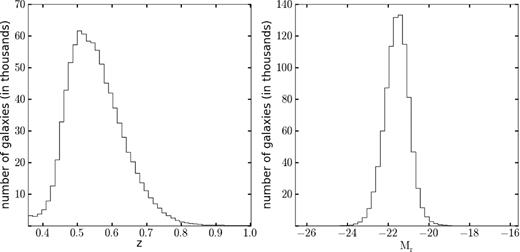
Redshift (left-hand panel) and luminosity (right-hand panel) distributions for the selected CMASS galaxies (see the text for details).

3 STACKING PROCEDURE

This section describes the method used to measure the average Mg ii absorption equivalent width as a function of impact parameter from the CMASS galaxies. In general, the mean transmission fraction |$\overline{F}$| of light from a background quasar due to Mg ii absorption line systems can be written as a function of the impact parameter r_p and velocity separation v from a galaxy, as

\begin{equation} \overline{F}(r_{\rm p},v)= \exp [-\tau _{\rm e}(r_{\rm p},v)]= \exp [ -\tau _{\rm e0}(1+\delta _{\mathrm{Mg}}(r_{\rm p},v)) ]. \end{equation}

(3)

Here, τ_e is the effective optical depth, and τ_e0 is its average value at any random position, irrespective of the presence of a galaxy. The perturbation δ_Mg is the relative increase of the effective optical depth of Mg ii absorption associated with the presence of a galaxy at impact parameter r_p and velocity separation v. The shape of this perturbation as a function of v, for a given impact parameter, is rather complicated because it arises from the distribution of relative velocities of a set of doublet lines with different degrees of saturation; besides, the observations are affected by the instrumental resolution and the binning. We will return to these details later.

The mean effective optical depth at a random position can be expressed in terms of the rest-frame equivalent width distribution of Mg ii absorbers, as

\begin{equation} \tau _{\rm e0}=\int _{0}^{\infty } {\rm d}W \, \frac{\mathrm{\partial} ^{2} \mathcal {N}}{\mathrm{\partial} W\mathrm{\partial} z}\, (1+z) \frac{W[1+\bar{q}(W)]}{\lambda _{\rm {Mg\,\small {II}}}}, \end{equation}

(4)

where the equivalent width W is that of the strongest line of the Mg ii doublet at λ = 2796.35 Å, and |$\bar{q}(W)$| is the mean equivalent width ratio of the two doublet lines.

Our aim in this paper is to measure the excess in the effective optical depth,

\begin{equation} \delta \tau _{\rm e}(r_{\rm p},v) = \tau _{\rm e}(r_{\rm p},v)-\tau _{\rm e0} = \tau _{\rm e0} \delta _{\mathrm{Mg}}(r_{\rm p},v), \end{equation}

(5)

which is induced by the presence of a galaxy at impact parameter r_p and velocity separation v. This quantity is directly related to the cross-correlation of Mg ii clouds with CMASS galaxies. We will focus in particular on the projected value of δτ_e, obtained after integration over velocity, and its relationship to the projected cross-correlation. The method we use to measure this cross-correlation is to average the transmitted fraction over a large number of lines of sight within a given range of impact parameter, in order to reduce the photon noise and the noise arising from quasar continuum variability.

A crucial step to measure the Mg ii–galaxy cross-correlation, in the form of δτ_e, is to estimate the quasar continuum with a method that is, to the best possible degree, free of systematic errors when averaging over a large number of lines of sight. In particular, it is important to ensure that the presence of a Mg ii line itself, which in most cases may be too weak to be individually detected in the relatively low S/N SDSS quasar spectra, does not bias the estimate of the continuum. Obviously, if the spectral region where we expect to find the Mg ii line associated with a galaxy is used for the continuum determination, the continuum estimate may be systematically biased too low because of the presence of an undetected Mg ii line. This systematic bias may be important when stacking large numbers of spectra, even though the Mg ii lines causing the bias are not individually detected in any single spectrum.

To illustrate the importance of the quasar continuum determination for the problem of measuring the average Mg ii absorption around galaxies at large impact parameters, we explore two different methods and we perform a number of tests for the presence of systematic errors. The first method, designated as mean subtraction, is specifically designed for our problem, while the second method, designated as variable smoothing, fits a continuum by iteratively smoothing the spectrum with a variable smoothing length to flexibly fit both emission lines and featureless continuum regions. The latter method uses the entire spectrum to determine the continuum, including the region where the associated Mg ii line is expected, and is therefore subject to the systematic error described above. We now describe each method in detail. Tests of the methods that show that the mean subtraction method correctly recovers the mean equivalent width and the variable smoothing method is subject to various systematic errors, including the continuum fitting bias mentioned above, are presented in Appendix A.

3.1 Method 1: mean subtraction

The first approach uses the mean spectrum of all quasars as a continuum fit model. Each quasar spectrum is divided by the mean quasar spectrum, and then a linear fit to this ratio is obtained around the spectral region of the expected Mg ii line for each galaxy–quasar pair, but without using the narrower central interval where the Mg ii line should be located. This linear fit is used to further improve the continuum estimate, allowing for intrinsic variations of the quasar continua. The results are then stacked for all quasar–galaxy pairs at each interval of impact parameter, after shifting to the redshift of the galaxy in each pair, to obtain the final composite Mg ii absorption spectrum. We now explain each of these steps in detail.

3.1.1 Generating the mean spectrum

The mean quasar spectrum is generated using the DR7 quasar spectra following a similar approach as the one undertaken by Vanden Berk et al. (2001). The mean spectrum in Vanden Berk et al. (2001) was generated using 1800 quasars (fig. 3 of Vanden Berk et al. 2001), so our mean spectrum is more accurate because of the much larger number of quasars available in DR7. In addition, we normalize the spectra using a spectral window that is particularly suited to obtaining the most accurate continuum model in the region where Mg ii absorption lines are found. There is therefore a small difference between our mean spectrum and that of Vanden Berk et al. (2001).

The quasar spectra are first shifted to the rest frame, using the redshifts of Schneider et al. (2010), and rebinned into a common wavelength scale of 1 Å per bin, which is close to the resolution of the observed spectra when shifted to the rest frame. The values of the flux and the error at each pixel in the new binning are determined by the average values of the flux and error in the original pixels that are projected, partly or fully, to the new pixel, weighted by the fraction of the new bin covered by each original bin. Each quasar spectrum, denoted by an index j, is normalized with a normalizing factor n_j equal to the mean flux in the interval 2000–2600 Å,

\begin{equation} n_j = \sum _{i}f_{ij}/N_j, \end{equation}

(6)

where f_ij is the measured flux value at pixel i of spectrum j, and N_j is the number of pixels in the rest-frame wavelength interval 2000 < λ_ij(1 + z_j) < 2600 Å. Any quasar spectra that do not cover this entire range of rest-frame wavelength are discarded. The final number of quasar spectra that are averaged in each 1 Å bin is shown in Fig. 2. The flat top corresponds to the spectral window used to compute the normalizing factor n_j. Note that the total number of quasar spectra used in this method is 70 650. The maximum number of quasars shown in Fig. 2, roughly 68 600 quasars, is lower than the total number of spectra used because we remove pixels affected by sky lines. Even though these sky lines are corrected by the BOSS pipeline, the noise in the affected pixels may sometimes not be well characterized, so it is best to remove these pixels. For each sky line, we remove a set of neighbouring pixels following the algorithm summarized in Palanque-Delabrouille et al. (2013) (for a more detailed explanation of the algorithm refer to Lee et al. 2013).

Figure 2.

Open in new tab Download slide

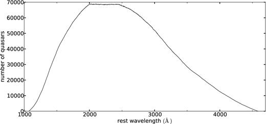
Number of quasar spectra contributing to each 1 Å bin of the mean spectrum, as a function of rest-frame wavelength. The flat feature corresponds to the spectral range used to compute the normalizing factor n_j. Outside this range the number of quasars contributing to the mean quasar spectrum decreases because some of the quasar spectra do not extend to that wavelength.

The rest-frame wavelength interval of 2000–2600 Å is also used to assign a mean S/N s_j to each spectrum, calculated as

\begin{equation} s_j = \frac{\sum _{i}f_{ij}/N_j}{\left(\sum _{i}e_{ij}^{2}/N_j\right)^{1/2}}, \end{equation}

(7)

where e_ij is the noise of the flux f_ij. The mean, normalized quasar spectrum is then obtained as a weighted average of all the quasar spectra

\begin{equation} \overline{f}_i = \frac{\sum _j\,w_j (f_{ij}/n_j)}{\sum _j\,w_j}, \end{equation}

(8)

where the weights w_j are set equal to

\begin{equation} w_j = \frac{1}{s_j^{-2}+\sigma _{I}^{2}}. \end{equation}

(9)

The constant σ_I is introduced to avoid the highest S/N spectra from excessively contributing to the final average, taking into account the presence of intrinsic quasar spectral variability, while reasonably weighting down the more noisy spectra. We fix this constant to σ_I = 0.05 (a reasonable estimate for the typical fractional intrinsic variability) throughout this paper. The resulting mean spectrum is shown in Fig. 3.

Figure 3.

Open in new tab Download slide

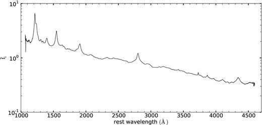
Mean spectrum of the weighted-average obtained from the 70 650 DR7 quasars, normalized in the rest-frame wavelength interval from 2000 to 2600 Å. This mean spectrum is used as a continuum model.

3.1.2 Generating the composite Mg ii absorption spectra

The composite Mg ii absorption spectra are obtained by stacking the spectra of all the quasars having a galaxy within the corresponding impact parameter bin, after being shifted to the rest frame of the galaxy in the region around the Mg ii doublet wavelength. For each quasar–galaxy pair, the quasar spectrum is first rebinned in a velocity variable v, defined in terms of the wavelength separation from the Mg ii absorption line in the rest frame of the galaxy at redshift z_gal,

\begin{equation} v = c\cdot \frac{\lambda -\lambda _{0}}{\lambda _{0}}, \end{equation}

(10)

where |$\lambda _{0}=\lambda _{\rm Mg\,\small {II}}(1+z_{\rm gal})$| and |$\lambda _{\rm Mg\,\small {II}} = 2798.743\, {^{\circ}_{\rm A}}$|⁠. We use the same linear rebinning method described in Section 3.1.1, with a bin size |$\Delta v = 50\, {\rm \, {\rm km}\, {\rm s}^{-1} }$|⁠. The mean spectrum is also rebinned in the same manner, but using |$\lambda _{0}=\lambda _{\rm Mg\,\small {II}} (1+z_{\rm gal})/(1+z_{\rm q})$|⁠, where z_q is the quasar redshift, because the mean quasar spectrum is computed in the quasar rest frame.

The rebinned spectra |$f^{(r)}_{ik}$|⁠, where the i index now labels the new bins in v and the k index labels each quasar–galaxy pair in a certain impact parameter bin, are then divided by the continuum to obtain a first estimate of the transmission fraction |$F^{(0)}_{ik}$|⁠,

\begin{equation} F^{(0)}_{ik}=\frac{f^{(r)}_{ik}/n_{j(k)}}{\overline{f}_{i}}, \end{equation}

(11)

where the normalization factor n_j(k) is that of the j quasar corresponding to each pair k. The mean quasar spectrum |$\overline{f}$| is understood to be the rebinned one and evaluated at the same bins in v for each quasar–galaxy pair. Hence, if all quasars had identical intrinsic emission spectra, and in the absence of intervening absorption and observational noise, this transmission would be equal to unity for all quasars. The errors are normalized in the same way and computed according to |$E_{ij} = e_{ij}/n_{j}/\overline{f}_{i}$|⁠.

In order to account for intrinsic variations in the spectra of quasars, we allow for a local smooth gradient in the ratio of each quasar spectrum to the mean spectrum in the region around each expected Mg ii absorption line. This is modelled by first calculating a weighted average value of |$F^{(0)}_{ik}$| on two intervals in v on each side of the expected Mg ii absorption associated with the galaxy, which are far enough from the centre so that any associated absorption can be neglected. The intervals used throughout this paper are −5000 km s⁻¹ < v < −2000 km s⁻¹ and 2000 km s⁻¹ < v < 5000 km s⁻¹, with their weighted averages designated as |$F^{(-)}_k$| and |$F^{(+)}_k$|⁠, respectively. The weights for each bin are set to |$w_{ik}=(\sigma _{n,ik}^2+\sigma _I^2)^{-1}$|⁠, where |$\sigma _{n,ik}=E_{ik}/F^{(+,-)}_k$| is the inverse S/N at each pixel (we use the averages |$F^{(+)}_k$| and |$F^{(-)}_k$| for the signal, instead of the values at each pixel |$F^{(0)}_{ik}$|⁠, to avoid biasing the result by systematically giving higher weights to pixels with positive noise). We use, as before, σ_I = 0.05. Weighted averages of the mean velocities |$v^{(-)}_k$| and |$v^{(+)}_k$| are computed in the same manner, which are usually close to the central values of the intervals (−3500 and +3500 km s⁻¹), but not exactly so. A linear function L_ik matching these two points is then defined as

\begin{equation} L_{ik}= F^{(-)}_k + \left(F^{(+)}_k - F^{(-)}_k\right)\left(v_i-v^{(-)}_k\right) / \left(v^{(+)}_k-(v^{(-)}_k\right). \end{equation}

(12)

In order to better adjust the quasar continuum in the presence of unrelated random absorption lines or bad pixels, the calculation of the two weighted averages |$F^{(-)}_k$| and |$F^{(+)}_k$| is recomputed after eliminating all outlier pixels in which the normalized flux deviates by more than 3σ from the fitted linear function, i.e. pixels where |$\Vert F^{(0)}_{ik}-L_{ik} \Vert > 3(\sigma _{n,ik}^{2}+\sigma _{I}^{2})^{1/2}$|⁠. If more than 20 per cent of the pixels in any of the two intervals are rejected under this criterion, the quasar spectrum is considered anomalous in the region of the expected Mg ii line and the quasar–galaxy pair under consideration is rejected and not included in the final processing.

The transmission fraction is then corrected by this linear fit as

\begin{equation} F_{ik} = F^{(0)}_{ik}+\left(1-L_{ik}\right). \end{equation}

(13)

We note here that although it would be in principle more correct to divide by the linear fit, setting |$F_{ik} = F^{(0)}_{ik}/L_{ik}$|⁠, we found that this procedure inevitably introduces a systematic feature in the final stacked spectrum owing to the fact that a Gaussian error in the function L results in a non-Gaussian distribution of the final transmission F when L is in the denominator, which is very difficult to correct for. We therefore decided to subtract L following equation (13).

Finally, we use the same weights as in equation (9) to compute the final composite spectrum and its errors,

\begin{equation} \overline{F}_i = \frac{\sum _{k}F_{ik}w_{j(k)}}{\sum _{k}w_{j(k)}} ; \qquad \overline{E}_{i}^{-2} = \frac{\sum _{k}E_{ik}^{-2}w_{j(k)}}{\sum _{j}w_{j(k)}}. \end{equation}

(14)

The index j(k) refers to the quasar index j corresponding to each quasar–galaxy pair labelled by the index k. In these sums, any pixels over the interval from −5000 to +5000 km s⁻¹ with a normalized flux F_ik below −2 or above +3 are eliminated, to exclude bad pixels or values that may have excessive noise. This eliminates only 0.02 per cent of the pixels.

The whole procedure is illustrated in Fig. 4 with a couple of examples, one with an individually detected Mg ii absorption system and one without any individually detected Mg ii absorption but with a random metal absorption line. Note that the contribution of these random metal absorption lines is later corrected for (Section 3.3).

Figure 4.

$Examples illustrating the procedure explained in Section 3.1.2. The left-hand column shows a case with a detected individual Mg ii absorption system, and the right-hand column a case with no detectable associated Mg ii absorption system, but with an unrelated metal absorption line. The top panels show the normalized flux of the spectral region, $f^{(r)}_{ik}/n_{j(k)}$ (solid blue line), and the normalized mean spectrum $\overline{f}_{i}$ (dashed red line). The bottom panels show the transmission $F^{(0)}_{ik}$ (thin, solid red line), the computed linear fit Lik (thin, dashed red line), and the corrected transmission Fik (thick, solid blue line). In the bottom right-hand panel, the points indicate pixels that are excluded from the linear fit. A horizontal thick dashed green line at a transmission of 1 is included for visual aid.$

Open in new tab Download slide

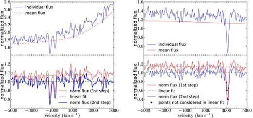
Examples illustrating the procedure explained in Section 3.1.2. The left-hand column shows a case with a detected individual Mg ii absorption system, and the right-hand column a case with no detectable associated Mg ii absorption system, but with an unrelated metal absorption line. The top panels show the normalized flux of the spectral region, |$f^{(r)}_{ik}/n_{j(k)}$| (solid blue line), and the normalized mean spectrum |$\overline{f}_{i}$| (dashed red line). The bottom panels show the transmission |$F^{(0)}_{ik}$| (thin, solid red line), the computed linear fit L_ik (thin, dashed red line), and the corrected transmission F_ik (thick, solid blue line). In the bottom right-hand panel, the points indicate pixels that are excluded from the linear fit. A horizontal thick dashed green line at a transmission of 1 is included for visual aid.

3.2 Method 2: variable smoothing

As a second approach to determine the continuum, we use the method described in York et al. (2005), based on an iterative smoothing of the spectrum with a variable smoothing length that is adjusted to decrease in spectral regions of known quasar emission lines. Each quasar spectrum is normalized by dividing both the flux and error by the variable smoothing continuum model, c_ij:

\begin{equation} F^{\prime }_{ij}=f_{ij}/c_{ij} ; \qquad E^{\prime }_{ij}=e_{ij}/c_{ij}. \end{equation}

(15)

In the same way as for the first method, the normalized spectra are rebinned into the variable v with bin width of 50 km s⁻¹. The final composite spectrum is calculated using the same weights as in equation (9), following equation (14), but using the primed variables |$F^{\prime }_{ij}$| and |$E^{\prime }_{ij}$|⁠.

3.3 Unbiasing the composite spectra

After the stacking of all the normalized spectra of quasar–galaxy pairs as a function of the velocity variable v has been completed by using either continuum fitting method, the mean value of the transmission |$\bar{F}_i$| that is obtained far from the expected Mg ii line (i.e. at large values of ‖v‖) is close to unity but not exactly so. The main reason for this is the presence of random metal absorption lines (unrelated to the galaxy of the pair) that are detected above a 3σ fluctuation and therefore excluded when fitting the continuum. Other reasons may be affecting this mean background of |$\overline{F}_i$| related to systematic effects in the noise distribution and the continuum fitting method. We eliminate this bias by performing the same linear fit to the stacked spectrum as in Section 3.1.2, using again the velocity intervals (−5000, −2000) and (2000, 5000) km s⁻¹ to measure two average values of |$\overline{F}_i$|⁠, and obtaining a linear fit based on two points at the centre of these intervals. The final normalized stacked flux is found by dividing by this linear fit.

Our results will actually be shown, for convenience, in terms of the effective excess optical depth, defined according to |$\delta \tau _{{\rm e},i} = - \log \bar{F}_i$|⁠, in Figs 5 to 7.

Figure 5.

Open in new tab Download slide

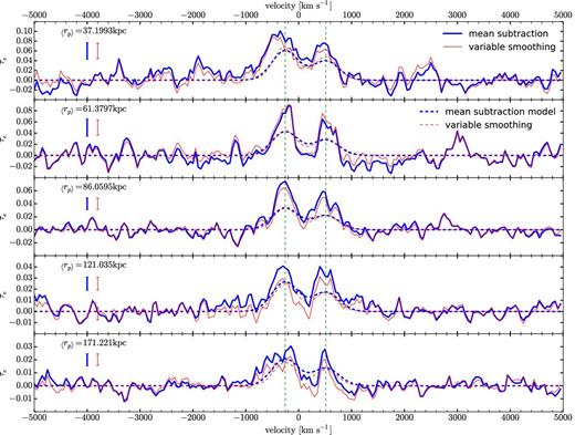
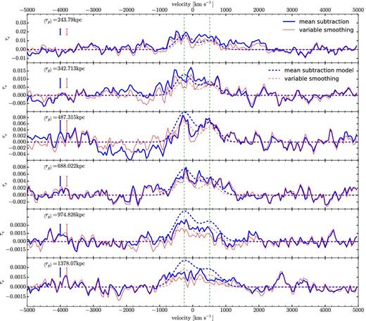
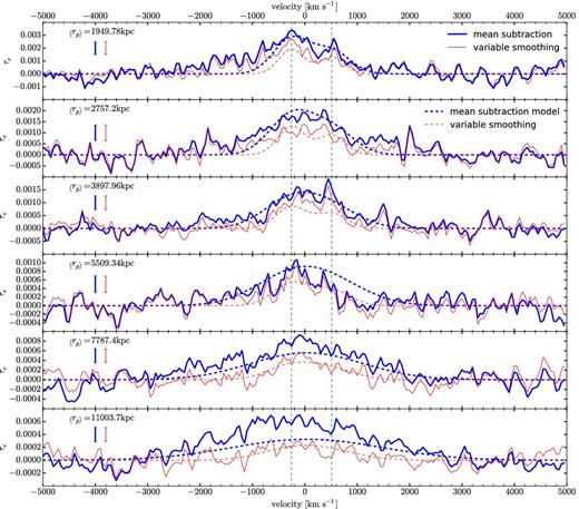
From top to bottom, composite spectra for increasing impact parameter intervals (in proper kpc). The effective optical depth is shown against velocity for the mean subtraction method (thick, solid blue line) and the variable smoothing method (thin, solid red line). The rms value of the bootstrap error in individual pixels is shown by the error bars on the left. The thick, dashed blue line and the thin, dashed red line are the best-fitting models (equation 16) for the mean subtraction and variable smoothing methods, respectively. A single set of parameters are fitted to all the 17 regions. Figs 6 and 7 show the spectra for the remaining impact parameter intervals. The stacks show a mean absorption profile for the presence of the Mg ii doublet line at the expected position. For visual guidance, vertical, dashed green lines mark the predicted position of the Mg ii doublet.

3.4 Bootstrap errors

The errors computed from the known observational noise in the observed quasar spectra that are stacked are actually a lower limit to the true errors. In reality, the intrinsic variability of real quasar continua and of the associated Mg ii and other random metal absorption lines imply the presence of additional errors that are not taken into account and which are correlated among the pixels of the final stacks. We therefore compute bootstrap errors, which are generally used in our analysis and model fits in this paper.

To calculate these bootstrap errors, we use the BOSS plates as the regions of the sky in which the sample is divided. Each quasar is tagged with the plate number at which its best spectrum was observed. For DR7 there are N_plates = 1822 plates. Pairs are counted as belonging to the plate that contains the quasar, irrespective of the galaxy position.

Bootstrap errors are computed in the standard way, generating N = 1000 samples by randomly selecting N_plates among all the plates with repetition, and then recalculating the composite spectra using both methods. Bootstrap errors are assigned to the final effective optical depth τ_e, at each velocity bin and each impact parameter interval from the dispersion found among the 1000 random samples. These bootstrap errors are computed for both continuum fitting methods.

We note that, specially at large impact parameter, some galaxies will be paired to quasars in different plates. This implies the presence of residual correlations among the bootstrap samples because of the common galaxies in pairs belonging to different plates, but we believe this effect is negligibly small because the most important error correlations should arise from the quasar spectra.

4 MODEL FOR THE ABSORPTION PROFILE

The usual analysis in the astronomical literature of individual Mg ii absorption lines is done by fitting with Voigt profiles, with the equivalent width and the velocity dispersion as free parameters. Whenever the observed absorption profile is not adequately fitted in terms of the two Voigt profiles of the Mg ii doublet, one can include the presence of multiple cloud components with blended absorption lines in order to improve the fit. Here, we are analysing a stack of a large number of Mg ii absorption systems that may be mostly undetected individually, but for which we can accurately predict the expected mean position from the redshift of the galaxy near the quasar line of sight. The effective optical depth in the stack, |$\tau _{\rm e} = -\log (\bar{F})$|⁠, should in this case have a single symmetric component for each line in the doublet, with a profile reflecting the velocity dispersion of Mg ii absorbing clouds and galaxies in haloes, as well as the large-scale halo correlation in redshift space for large impact parameters. This cross-correlation function can be modelled in terms of the halo occupation distribution formalism (e.g. Gauthier, Tinker & Chen 2008; Zhu & Ménard 2013a), but the density profile of Mg ii clouds in haloes does not have to follow that of galaxies, and it will generally depend on complex physics of galaxy winds and gas accretion in the circumgalactic medium. For simplicity, we shall assume in this section a model with a Gaussian velocity distribution and a power-law form for the projected correlation function, as an approximation to the generally complex form of the galaxy-absorber cross-correlation function. In the next section, we shall use a more accurate form of the correlation function obtained from halo simulations to determine the amplitude of our measured cross-correlation.

Our model has four free parameters. The first three are the central effective optical depth τ₀ of the strongest line in the doublet at a conventional normalization value of the impact parameter r_p0 (set here to 1 Mpc), the power-law slope α of the projected cross-correlation, and the mean equivalent width ratio q (where q = 1/2 if all the absorption lines were unsaturated, and q = 1 in the saturated case). We consider a variation of the velocity dispersion σ with radius, taking into account that in the limit of large radius, the Hubble expansion should lead to a linear increase of the effective dispersion. The fitted profile of the excess effective optical depth, δτ_e(b, v) (as defined in equation 5), is

\begin{eqnarray} \delta {\tau }_{\rm e}(r_{\rm p},v) &=& \frac{\tau _{0}}{\sqrt{1+(xHr_{\rm p}/\sigma _{0})^{2}}} \left( \frac{r_{\rm p}}{r_{\rm p0}}\right)^{-\alpha }\nonumber \\ &&\times \, [{\mathrm{e}}^{-\left(v-v_{1}\right)^{2}/2\sigma ^{2}} + q\, {\mathrm{e}}^{-\left(v-v_{2}\right)^{2}/2\sigma ^{2}}], \end{eqnarray}

(16)

where

\begin{equation} \sigma ^{2}=\sigma _{0}^{2}+(xHr_{\rm p})^{2}. \end{equation}

(17)

The fourth model parameter is therefore the dimensionless constant x, which is the scale at which the velocity dispersion starts to increase, compared to σ₀/H, with H(z = 0.55) = 91.7. In principle, the central velocity dispersion σ₀ should also be left as a free parameter, but in this paper we have fixed it to 250 km s⁻¹. The reason is that if this condition is relaxed, the obtained fits have a large degeneracy in σ₀ and x and they are largely dominated by an excess of absorption that is found at the largest impact parameters that we do not fully understand, as we shall see below. The value of 250 km s⁻¹ allows us to fit well the width of the doublet line at small impact parameter, where it is resolved. Note that the parameter q is assumed to be independent of impact parameter, even though it may generally depend on it (the mean saturation should decrease with impact parameter if the mean absorber equivalent width also decreases, as suggested by observations; e.g. Gauthier et al. 2009; Chen et al. 2010a). Note also that the instrumental point spread function (Smee et al. 2013) and finite spectral bin size is effectively included in the value of the velocity dispersion in our model. A more detailed modelling of these effects is neglected here for simplicity. The origin of the velocity coordinate v is chosen by convention as the central position of the Mg ii doublet for an unsaturated line (q = 0.5) at the redshift of the galaxy. Under this convention, v₁ = −256.05 km s⁻¹ and v₂ = 513.28 km s⁻¹.

The fitting is performed by χ² minimization, computed including all the pixels of the stacked spectra in the central interval |v| < 2000 km s⁻¹. Each pixel is weighted according to the bootstrap error measured in that pixel as described in Section 3.4, but without considering the cross-correlations of the errors between pixels. In practice, the bootstrap error bars in different pixels of the stacked spectra are nearly equal. The spectrum outside the interval |v| < 2000 km s⁻¹, which is used for deriving the continuum fit in Method 1, is not considered here for the fit. We note also that for a real Gaussian profile for each component of the Mg ii doublet, the continuum fitting of Method 1 implies that we formally need to subtract a small constant from the double Gaussian in equation (16), equal to the integrated value of the model absorption over the interval v ∈ (2000, 5000) km s⁻¹ used for determining the continuum, but we neglect this effect here.

We use a Markov chain Monte Carlo method to perform the χ² minimization to the five-parameter model fit. The errors of the parameters are also obtained by repeating the model fit with bootstrap realizations. The average integrated equivalent width as a function of impact parameter can be obtained directly by integrating the effective optical depth over the interval used to fit the model

\begin{equation} W_{\rm e}(r_{\rm p}) =\frac{\lambda _{\rm Mg\,\small {II}}}{c} \int _{-2000\, {\rm \, {\rm km}\, {\rm s}^{-1} }}^{2000\, {\rm \, {\rm km}\, {\rm s}^{-1} }}\, \delta {\tau }_{e}(r_{{\rm p}},v)\, \mathrm{d}v. \end{equation}

(18)

The fitted model also predicts a mean equivalent width

\begin{eqnarray} W_e(r_{{\rm p}}) &=& \frac{\lambda _{\rm Mg\,\small {II}}}{c} \sqrt{2\pi }\, \tau _{0}\sigma _{0} (1+q)\, \left(\frac{r_{{\rm p}}}{r_{{\rm p}0}}\right)^{-\alpha }\nonumber \\ &=& W_{e0} \left(\frac{r_{{\rm p}}}{r_{{\rm p}0}}\right)^{-\alpha }, \end{eqnarray}

(19)

although this value is for the absorption over the whole velocity range, not restricted to the interval −2000 km s⁻¹ < v < 2000 km s⁻¹.

5 RESULTS

The results of the stacked absorption profiles are obtained for a total of 17 impact parameter intervals, measured in proper units at the redshift of the galaxy. The first interval is for r_p < 50 kpc, and the other 16 intervals are 2^(i−1)/2 < (r_p/50 kpc) < 2^i/2, for i = 1 to 16, up to a maximum impact parameter of 12.8 Mpc. The stacked profiles are shown as the effective optical depth, |$\tau _{\rm e}=-\log (\bar{F})$|⁠, in Figs 5–7. Results are presented for our two continuum fitting methods, the mean subtraction method (thick, solid blue line) and the variable smoothing method (thin, solid red line). The error bars plotted on the left-hand side are the rms values of the bootstrap error of τ_e in one pixel, which has little variation among different pixels in each stacked spectrum. The results of the fitted model parameters and their bootstrap errors computed by repeating the fit for bootstrap realizations of the stacked profiles, are given in Table 1 (the cross-correlations of the parameter errors are omitted).

Figure 6.

Open in new tab Download slide

Continuation of Fig. 5.

Figure 7.

Open in new tab Download slide

Continuation of Fig. 5.

Table 1.

Best-fitting values for the fitted parameters of the model described in Section 4 and shown as the lines in Fig. 9. First column: results using the mean subtraction method (see Section 3.1). Second column: results using the variable smoothing method (see Section 3.2). Four independent parameters are fitted, and W_e0 is related to the other parameters according to equation (19). As explained in Section 4, σ₀ is fixed at 250 km s⁻¹. Errors are computed from repeating the fits on bootstrap realizations of the stacked profiles.

	Mean subtraction	Variable smoothing
τ₀	0.0060 ± 0.0001	0.0034 ± 0.0001
α	0.70 ± 0.01	0.88 ± 0.01
σ₀ ( km s⁻¹)	250	250
x	1.35 ± 0.06	0.46 ± 0.08
q	0.65 ± 0.03	0.66 ± 0.03
W_e0( km s⁻¹)	6.27 ± 0.10	3.58 ± 0.08

	Mean subtraction	Variable smoothing
τ₀	0.0060 ± 0.0001	0.0034 ± 0.0001
α	0.70 ± 0.01	0.88 ± 0.01
σ₀ ( km s⁻¹)	250	250
x	1.35 ± 0.06	0.46 ± 0.08
q	0.65 ± 0.03	0.66 ± 0.03
W_e0( km s⁻¹)	6.27 ± 0.10	3.58 ± 0.08

Open in new tab

Table 1.

Best-fitting values for the fitted parameters of the model described in Section 4 and shown as the lines in Fig. 9. First column: results using the mean subtraction method (see Section 3.1). Second column: results using the variable smoothing method (see Section 3.2). Four independent parameters are fitted, and W_e0 is related to the other parameters according to equation (19). As explained in Section 4, σ₀ is fixed at 250 km s⁻¹. Errors are computed from repeating the fits on bootstrap realizations of the stacked profiles.

	Mean subtraction	Variable smoothing
τ₀	0.0060 ± 0.0001	0.0034 ± 0.0001
α	0.70 ± 0.01	0.88 ± 0.01
σ₀ ( km s⁻¹)	250	250
x	1.35 ± 0.06	0.46 ± 0.08
q	0.65 ± 0.03	0.66 ± 0.03
W_e0( km s⁻¹)	6.27 ± 0.10	3.58 ± 0.08

	Mean subtraction	Variable smoothing
τ₀	0.0060 ± 0.0001	0.0034 ± 0.0001
α	0.70 ± 0.01	0.88 ± 0.01
σ₀ ( km s⁻¹)	250	250
x	1.35 ± 0.06	0.46 ± 0.08
q	0.65 ± 0.03	0.66 ± 0.03
W_e0( km s⁻¹)	6.27 ± 0.10	3.58 ± 0.08

Open in new tab

The stacks in Figs 5–7 show the mean absorption profile of the Mg ii doublet line, clearly seen at the expected positions at small impact parameters. The amplitude of the random pixel-to-pixel variations outside of the central absorption feature is generally consistent with the computed bootstrap error bars. The expected doublet feature of the Mg ii line is generally resolved at r_p ≲ 200 kpc, and is smoothed out at larger impact parameter by the velocity dispersion of the absorbers, which should increase linearly with r_p in the limit of large radius because of Hubble expansion. The fact that our parameter x is close to unity supports this interpretation, although we note that the precise expected theoretical value of x in the linear regime is not one because of redshift distortions. We do not analyse this issue further in this paper because the maximum impact parameter that we analyse is not yet in the linear regime, and a more detailed model would be necessary for the velocity distribution of absorbers as a function of impact parameter. We mention here that we initially considered a simpler model with x = 0 and σ₀ as free parameter, but this choice gave a substantially worse fit and resulted in a high value of the velocity dispersion because of its increase with radius. As mentioned previously, fits leaving both σ₀ and x₀ as free parameters lead to a substantial degeneracy and to solutions with very large values of σ₀, driven by the excess of absorption that is seen in the last r_p bin for the mean subtraction method. We have not found an explanation for this excess in the last bin, which is only marginally consistent (at the ∼3σ level, as shown in Fig. 8) with our fit.

A value q ≃ 0.65 is obtained for the line ratio of the Mg ii doublet, consistent with a mixture of saturated and unsaturated lines. It has been previously reported that the mean equivalent width of the Mg ii lines decreases with impact parameter (Gauthier et al. 2009, and references therein). This result may imply that absorbers are less saturated at larger impact parameters, and should therefore have a decreasing value of q, although this interpretation depends on whether the internal velocity dispersion of the absorbing clouds varies with impact parameter (note that this internal velocity dispersion is much smaller than the velocity dispersion of absorbing components around their host galaxies). Our model assumes a constant value of q for simplicity.

The mean equivalent widths obtained with our two methods, by directly integrating the effective optical depth in the stacked spectra as in equation (18), are shown in Fig. 8 as blue triangles for the mean subtraction method, and red squares for the variable smoothing method. These values and their bootstrap errors are also given in Table 2, together with the number of galaxy–quasar pairs that contribute to the stacked spectrum at each impact parameter bin. Note that this mean equivalent width is for the sum of the two lines in the Mg ii doublet. There is a systematic difference in the mean equivalent width obtained with the two methods; the variable smoothing method yields a systematically smaller equivalent width compared to the mean subtraction method, and the discrepancy increases with impact parameter, reaching more than a factor of 2 at r_p = 10 Mpc. As mentioned previously in Section 3, the reason for this difference is that the spectral region where Mg ii absorption is expected is used to determine the continuum in the variable smoothing method. The presence of weak lines that remain undetected in individual spectra causes the continuum to be underestimated in a way that depends on the S/N and the equivalent width of the undetected line in a complex manner. This systematic underestimate of the continuum causes the underestimate of the mean equivalent width. Appendix A presents quantitative tests demonstrating the presence of this systematic error of the variable smoothing method, and shows also that the result obtained with the mean subtraction method, which does not use the stacked spectrum in the region of the Mg ii absorption to determine the continuum, is free of any similar systematic effect to the extent that we are able to discern.

Figure 8.

Open in new tab Download slide

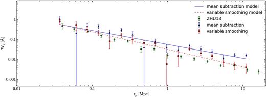
Measured rest-frame mean equivalent width W_e of the Mg ii doublet, versus proper impact parameter. The blue triangles are obtained from the mean subtraction continuum method, and red squares use the variable smoothing method. Error bars have been obtained by the bootstrap method. Lines are the best-fitting power-law model to the data for both methods. The green circles are the results of Zhu et al. (2013). Note that the results for the mean subtraction method are systematically higher than the rest. This is explored in further detail in Appendix A.

Table 2.

Results on the mean equivalent width and errors shown in Fig. 8, presented here as a table. From left to right, impact parameter interval, mean rest-frame Mg ii equivalent width and its bootstrap error for the mean subtraction and variable smoothing methods, and number of QSO–galaxy pairs used in the interval. The mean rest-frame equivalent widths are the sum of both lines in the doublet.

r_p	Mean subtraction		Variable smoothing		N_pairs
	〈W〉	σ(〈W〉)	〈W〉	σ(〈W〉)
(kpc)	(Å)	(Å)	(Å)	(Å)
(0, 50]	1.10	0.35	0.84	0.25	76
(50, 70.71]	0.22	0.40	0.54	0.25	94
(70.71, 100]	0.49	0.15	0.33	0.10	204
(100, 141.42]	0.48	0.12	0.230	0.074	423
(141.42, 200]	0.229	0.080	0.084	0.049	758
(200, 282.84]	0.317	0.058	0.168	0.041	1396
(282.84, 400]	0.181	0.076	0.102	0.042	2621
(400, 565.69]	0.042	0.049	0.069	0.028	4904
(565.69, 800]	0.081	0.029	0.069	0.019	9576
(800, 1131.37]	0.040	0.018	0.006	0.012	19 166
(1131.37, 1600]	0.032	0.015	0.015	0.010	38 922
(1600, 2262.74]	0.0506	0.0093	0.0354	0.0068	75 567
(2262.74, 3200]	0.0360	0.0072	0.0211	0.0051	148 769
(3200, 4525.48]	0.0258	0.0062	0.0152	0.0038	290 340
(4525.48, 6400]	0.0119	0.0044	0.0073	0.0028	559 840
(6400, 9050.97]	0.0180	0.0036	0.0053	0.0022	1062 482
(9050.97, 12800]	0.0169	0.0028	0.0041	0.0020	1961 450

r_p	Mean subtraction		Variable smoothing		N_pairs
	〈W〉	σ(〈W〉)	〈W〉	σ(〈W〉)
(kpc)	(Å)	(Å)	(Å)	(Å)
(0, 50]	1.10	0.35	0.84	0.25	76
(50, 70.71]	0.22	0.40	0.54	0.25	94
(70.71, 100]	0.49	0.15	0.33	0.10	204
(100, 141.42]	0.48	0.12	0.230	0.074	423
(141.42, 200]	0.229	0.080	0.084	0.049	758
(200, 282.84]	0.317	0.058	0.168	0.041	1396
(282.84, 400]	0.181	0.076	0.102	0.042	2621
(400, 565.69]	0.042	0.049	0.069	0.028	4904
(565.69, 800]	0.081	0.029	0.069	0.019	9576
(800, 1131.37]	0.040	0.018	0.006	0.012	19 166
(1131.37, 1600]	0.032	0.015	0.015	0.010	38 922
(1600, 2262.74]	0.0506	0.0093	0.0354	0.0068	75 567
(2262.74, 3200]	0.0360	0.0072	0.0211	0.0051	148 769
(3200, 4525.48]	0.0258	0.0062	0.0152	0.0038	290 340
(4525.48, 6400]	0.0119	0.0044	0.0073	0.0028	559 840
(6400, 9050.97]	0.0180	0.0036	0.0053	0.0022	1062 482
(9050.97, 12800]	0.0169	0.0028	0.0041	0.0020	1961 450

Open in new tab

Table 2.

Results on the mean equivalent width and errors shown in Fig. 8, presented here as a table. From left to right, impact parameter interval, mean rest-frame Mg ii equivalent width and its bootstrap error for the mean subtraction and variable smoothing methods, and number of QSO–galaxy pairs used in the interval. The mean rest-frame equivalent widths are the sum of both lines in the doublet.

r_p	Mean subtraction		Variable smoothing		N_pairs
	〈W〉	σ(〈W〉)	〈W〉	σ(〈W〉)
(kpc)	(Å)	(Å)	(Å)	(Å)
(0, 50]	1.10	0.35	0.84	0.25	76
(50, 70.71]	0.22	0.40	0.54	0.25	94
(70.71, 100]	0.49	0.15	0.33	0.10	204
(100, 141.42]	0.48	0.12	0.230	0.074	423
(141.42, 200]	0.229	0.080	0.084	0.049	758
(200, 282.84]	0.317	0.058	0.168	0.041	1396
(282.84, 400]	0.181	0.076	0.102	0.042	2621
(400, 565.69]	0.042	0.049	0.069	0.028	4904
(565.69, 800]	0.081	0.029	0.069	0.019	9576
(800, 1131.37]	0.040	0.018	0.006	0.012	19 166
(1131.37, 1600]	0.032	0.015	0.015	0.010	38 922
(1600, 2262.74]	0.0506	0.0093	0.0354	0.0068	75 567
(2262.74, 3200]	0.0360	0.0072	0.0211	0.0051	148 769
(3200, 4525.48]	0.0258	0.0062	0.0152	0.0038	290 340
(4525.48, 6400]	0.0119	0.0044	0.0073	0.0028	559 840
(6400, 9050.97]	0.0180	0.0036	0.0053	0.0022	1062 482
(9050.97, 12800]	0.0169	0.0028	0.0041	0.0020	1961 450

r_p	Mean subtraction		Variable smoothing		N_pairs
	〈W〉	σ(〈W〉)	〈W〉	σ(〈W〉)
(kpc)	(Å)	(Å)	(Å)	(Å)
(0, 50]	1.10	0.35	0.84	0.25	76
(50, 70.71]	0.22	0.40	0.54	0.25	94
(70.71, 100]	0.49	0.15	0.33	0.10	204
(100, 141.42]	0.48	0.12	0.230	0.074	423
(141.42, 200]	0.229	0.080	0.084	0.049	758
(200, 282.84]	0.317	0.058	0.168	0.041	1396
(282.84, 400]	0.181	0.076	0.102	0.042	2621
(400, 565.69]	0.042	0.049	0.069	0.028	4904
(565.69, 800]	0.081	0.029	0.069	0.019	9576
(800, 1131.37]	0.040	0.018	0.006	0.012	19 166
(1131.37, 1600]	0.032	0.015	0.015	0.010	38 922
(1600, 2262.74]	0.0506	0.0093	0.0354	0.0068	75 567
(2262.74, 3200]	0.0360	0.0072	0.0211	0.0051	148 769
(3200, 4525.48]	0.0258	0.0062	0.0152	0.0038	290 340
(4525.48, 6400]	0.0119	0.0044	0.0073	0.0028	559 840
(6400, 9050.97]	0.0180	0.0036	0.0053	0.0022	1062 482
(9050.97, 12800]	0.0169	0.0028	0.0041	0.0020	1961 450

Open in new tab

The green circles with error bars in Fig. 8 show the results of Zhu et al. (2013), who have used a sample of galaxies and quasar spectra similar to ours to infer the same mean equivalent width as a function of impact parameter. Their result is systematically below ours, roughly by a factor of ∼2 at all impact parameters, and is lower even compared to our variable smoothing method. We believe the reason is again due to the systematic underestimate of the continuum. The continuum fitting method used by Zhu et al. (2013) also uses the observed spectra in the region where Mg ii absorption is expected in a rather complex way that is described in Zhu & Ménard (2013b), and the systematic error that this induces is difficult to predict but may in principle explain why it produces a systematically low estimate of the equivalent width. Note that in principle this underestimation will only affect the individually undetected systems. Individually undetected systems cannot be distinguished from the noise and will thus be fitted away by the continuum fitter. Individually detected systems will, in principle, not suffer from this effect. The error bars of Zhu et al. (2013) are also smaller than ours, since their continuum fitting can better remove any features of the quasar spectrum that are superposed with the Mg ii absorption lines, at the cost of introducing a systematic bias in the continuum estimate.

6 DISCUSSION

6.1 Relation of the mean equivalent width to the bias factor of Mg ii absorption systems

Our measurement of the cross-correlation of Mg ii absorption systems and galaxies in the CMASS catalogue of BOSS clearly reflects properties of the spatial distribution of these two objects. In the limit of large scales, when the fluctuations are in the linear regime, any population of objects that traces the large-scale mass perturbations is characterized by its bias factor and the autocorrelation in real space is equal to the correlation function of the mass times the square of the bias factor, with redshift distortions added in redshift space (Kaiser 1987; Cole & Kaiser 1989). The cross-correlation of two classes of objects is, in the same large-scale limit, equal to the mass correlation function times the product of the two bias factors. On small, non-linear scales, the correlations are more complex and they depend on other physics that determine the distribution of galaxies and Mg ii absorbers in relation to dark matter haloes.

Our stacked spectra measure the mean excess of the effective optical depth as a function of impact parameter r_p and velocity separation v from a galaxy. This quantity is related to the mean Mg ii absorption perturbation, δ_Mg(r_p, v), as

\begin{equation} \tau _{\rm e}(r_{\rm p},v)=\tau _{\rm e0}(1+\delta _{\mathrm{Mg}}(r_{\rm p},v)), \end{equation}

(20)

where τ_e0 is the mean Mg ii effective optical depth, defined in equation (4). This perturbation is equal to the cross-correlation function of Mg ii absorbers and galaxies, convolved with the mean doublet absorption profile of a Mg ii system, and is the function that is measured in our stacking results in Figs 5 and 6. In this work, our interest is focused on the projected correlation function, related to the integrated absorption W_e(r_p) in equation (18). The projected cross-correlation is not affected by redshift distortions and by the complications arising from the convolution with the mean doublet line profile and the spectrograph resolution.

Here, we shall make two approximations to physically interpret our measurement of W_e(r_p): first, we neglect the effect of the finite integrating range ±2000 km s⁻¹ that we have used, ignoring the difference from the true projected correlation that is obtained by integrating to infinity. This approximation is likely not very good for the largest impact parameters we use; we discuss this further below. Secondly, we assume that the cross-correlation of Mg ii systems and CMASS galaxies is the same as the autocorrelation of CMASS galaxies times the ratio of bias factors b_Mg/b_g of the two types of objects. In other words, we assume the linear relation can be extended into the non-linear regime as far as the ratio of the cross-correlation to the autocorrelation is concerned.

This second assumption can be justified from observations of the correlations of galaxies of different luminosity. Zehavi et al. (2011) measured the projected correlation of galaxies in the DR7 catalogue in different luminosity ranges, and, to a good approximation, in the impact parameter range of our interest, the result is a fixed shape times the variable bias factor, as seen for example in their fig. 6. The shape of the galaxy correlation can be interpreted as arising from the correlation among virialized haloes and the distribution of galaxies within each halo (e.g. Zheng et al. 2005). This shape does vary slightly with luminosity, but the most important variation is the normalization determined by the bias factor. There is a greater variation of the shape of the projected correlation with galaxy colour (see fig. 21 in Zehavi et al. 2011). In addition, the projected cross-correlation of galaxies of different colour is not exactly equal to the geometric mean of the projected autocorrelations of the two types of galaxies (see their fig. 15). Our assumption can only be considered as a first approximation that will need to be tested in the future, but it allows us to obtain a bias factor for Mg ii absorption systems assuming that they behave in a similar way as galaxies in the CMASS catalogue.

These assumptions lead to the relation

\begin{eqnarray} W_{\rm e}(r_{\rm p}) &=& \frac{\tau _{\rm e0}\lambda _{\rm Mg\,\small {II}}}{c} \int {\rm d}v \, \delta _{\mathrm{Mg}}(r_{\rm p},v)\nonumber \\ &=&\frac{\lambda _{\rm Mg\,\small {II}}}{c} {\tau _{\rm e0}\, H(z)\over 1+z}\, \frac{b_{\mathrm{Mg}}}{b_{\rm g}}\, w_{\rm gg}(r_{\rm p}), \end{eqnarray}

(21)

where w_gg(r_p) is the projected galaxy correlation function, b_g is the galaxy bias factor and b_Mg is the mean bias factor of Mg ii absorption systems, weighted in proportion to their equivalent width. We have used dv = H(z)/(1 + z) dx, where dx is the comoving space coordinate that is integrated to obtain the projected galaxy correlation function, and z is the mean redshift of the galaxies and associated Mg ii absorption systems. This relation allows us to infer the bias factor of Mg ii systems empirically, using only the directly measured projected galaxy correlation. Its validity is strictly valid in the limit of large scales, but, as we shall see below, the ratio W_e(r_p)/w_gg(r_p) is roughly constant, making our assumption plausible as a first approximation.

6.2 Mean absorption from Mg ii systems

The value of τ_e0, representing the average absorption from the population of Mg ii absorbers, must be independently known before we can use the measured mean excess of Mg ii absorption around galaxies to infer the bias factor of Mg ii systems with equation (21). This parameter can be estimated from equation (4) using models of the equivalent width distribution that fit the observational data.

We use the double exponential model of Nestor et al. (2005)

\begin{equation} \frac{\mathrm{\partial} ^{2} \mathcal {N}}{\mathrm{\partial} W\mathrm{\partial} z} = \frac{N^{*}_{\rm wk}}{W^{*}_{\rm wk}}\exp ^{-W/W^{*}_{\rm wk}} + \frac{N^{*}_{\rm str}}{W^{*}_{\rm str}}\exp ^{-W/W^{*}_{\rm str}}, \end{equation}

(22)

where |$N_{\rm str}^{*}$| and |$N_{\rm wk}^{*}$| are the number of absorbers per unit of redshift in the strong and weak population, and |$W_{\rm str}^{*}$| and |$W_{\rm wk}^{*}$| are the characteristic rest-frame equivalent widths of the two exponential distributions. This model was fitted by Nestor et al. (2005) to their data, using mocks to correct for incompleteness at low equivalent widths. More recently, a compilation of high-resolution data was shown by Bernet, Miniati & Lilly (2010) in their fig. 5, reaching down to lower equivalent widths. We include these observational results in Fig. 9, overplotting the fit that was obtained by Nestor et al. (2005), which has the following parameters: |$N^{*}_{\rm wk}=1.71\pm 0.02$|⁠, |$W^{*}_{\rm wk}=0.072\pm 0.001$| Å, |$N^{*}_{\rm str}=0.932\pm 0.011$| and |$W^{*}_{\rm str}=0.771\pm 0.014$| Å. The observations are well reproduced by this fit, which we therefore use to compute τ_e0.

Figure 9.

Open in new tab Download slide

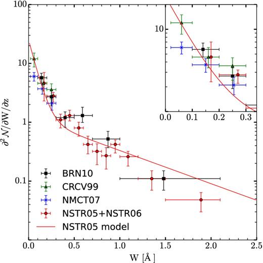
Rest-frame equivalent width distribution of Mg ii absorption systems. Data points are from Bernet et al. (2010) (black squares), Churchill et al. (1999) (green triangles), Narayanan et al. (2007) (blue crosses), and Nestor et al. (2005) and Nestor, Turnshek & Rao (2006) (red circles). The overplotted solid line is the double exponential fit of Nestor et al. (2005) (see the text). Top-right panel is a zoomed view of the weakest absorption systems.

Unfortunately, the sample of absorbers of Nestor et al. (2005) is somewhat heterogeneous, and the main uncertainty we encounter in using it to compute τ_e0 is due to the redshift evolution. A fit to this evolution was determined by Nestor et al. (2005), where the parameters of the exponential model vary as W* ∝ (1 + z)^0.634±0.097 and N* ∝ (1 + z)^{0.226 ± 0.170}, both for the weak and strong populations. We infer from their model fits and the mean value of N* that the mean redshift of their sample is z ≃ 1.1 and we use these relations to convert the product N*W* to the mean redshift of the CMASS galaxy catalogue, z ≃ 0.55. We find |$N_{\rm str}^{*} W_{\rm str}^{*} = 0.55$| Å and |$N_{\rm wk}^{*} W_{\rm wk}^{*} = 0.095$| Å, with an error that is close to 10 per cent, although it is poorly defined because the errors in the redshift evolution of |$N_{\rm str,wk}^{*}$| and |$W_{\rm str,wk}^{*}$| should be correlated, and this information (and the exact redshift distribution of the absorbers) was not provided in Nestor et al. (2005).

From equation (4), we derive the value of τ_e0 in the double exponential model of equation (22),

\begin{equation} \tau _{\rm e0} = \frac{1+z}{\lambda _{\rm {Mg\,\small {II}}}}\, (1+\bar{q})\, \left(N_{\rm wk}^{*}W_{\rm wk}^{*}+N_{\rm str}^{*}W_{\rm str}^{*} \right), \end{equation}

(23)

which yields a value τ_e0(z = 0.55) = 5.0 × 10⁻⁴, with an error of about 10 per cent but which is subject to uncertainties owing to the redshift evolution, the accuracy of the fit to the equivalent width distribution, and the value of |$\bar{q}$|⁠. Our results will be given in terms of τ_e0 without including its error, with the understanding that this quantity will need to be better determined in the future from studies of the field population of Mg ii absorbers.

6.3 Derivation of the bias factor of Mg ii systems

We now use equation (21) to infer the bias factor of the Mg ii systems, as

\begin{equation} b_{\mathrm{Mg}}= b_{\rm g}\, \frac{c\, W_{\rm e}(r_{\rm p})(1+z)}{\tau _{\rm e0}\lambda _{\rm Mg\,\small {II}}\, w_{\rm gg}(r_{\rm p})\,\, H(z)} . \end{equation}

(24)

Note that the factor (1 + z)/H(z) appears because of our convention that the effective equivalent width W_e is measured in Å, whereas w_gg is assumed to have been transformed to comoving length units. Instead of fitting our Mg ii–galaxy cross-correlation measurement with a power-law dependence with impact parameter (as in equation 16), we can directly fit the functional form that is determined from the observed projected galaxy correlation function, assuming that the shape is the same. To do this, we use the projected galaxy autocorrelation function obtained in Nuza et al. (2013) from the BOSS DR9 catalogue of CMASS galaxies, and their prediction for the galaxy correlation function based on assigning galaxies to haloes and subhaloes in their MultiDark simulation. The measurements of Nuza et al. (2013) are represented as the black triangles with error bars in Fig. 10, and their model is shown as the thick black line (given in their fig. 6 and table B1; note that we have corrected for the different cosmological model they use, with a present matter density Ω_m = 0.27 instead of our value Ω_m = 0.3). The blue triangles, red squares and green circles are the mean equivalent width W_e(r_p) times the factor (1 + z)/H(z)/τ_e0 (equal to the cross-correlation of Mg ii systems and CMASS galaxies), times r_p(1 + z) for the mean subtraction method, the variable smoothing method and measurements from Zhu et al. (2013), respectively.

Figure 10.

Open in new tab Download slide

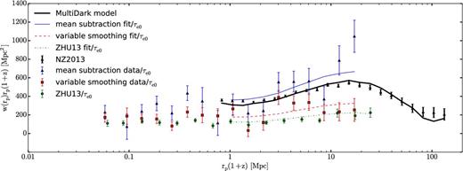
Projected correlation functions multiplied by the comoving impact parameter as a function of the comoving impact parameter r_p(1 + z). The thick black triangles with error bars show the autocorrelation of CMASS galaxies from Nuza et al. (2013). The blue triangles, red squares and green circles are the mean equivalent width W_e(r_p) times the factor (1 + z)/H(z)/τ_e0 (equal to the cross-correlation of Mg ii systems and CMASS galaxies), times r_p(1 + z) for the mean subtraction method, the variable smoothing method and measurements from Zhu et al. (2013), respectively. The thick solid black line is the MultiDark model prediction described in Nuza et al. (2013). The solid blue, the red dashed and the green dash–dotted lines are the fit to W_e for the mean subtraction method, the variable smoothing method and measurements from Zhu et al. (2013), respectively. The ratio of the each of these lines with the thick solid black line is the ratio of bias factors, b_Mg/b_g.

The galaxy bias factor in the model of Nuza et al. (2013) shown as the dashed black line is b_g = 2.00 ± 0.07. Note that this value is lower than that obtained by Guo et al. (2013), b_g = 2.16 ± 0.01, for the average CMASS galaxy. Using the value given by Guo et al. (2013) would lead to a larger measured value of the bias factor of the Mg ii systems. As explained in Guo et al. (2013), the value of the galaxy bias increases with luminosity and redshift, and it can also depend on the range of scales used to fit its value. Here, we use the galaxy bias value and the projected galaxy autocorrelation function of Nuza et al. (2013), but the discrepancy with the higher value obtained by Guo et al. (2013) needs to be resolved to remove this source of uncertainty on the derived bias value of the Mg ii absorption systems.

We now redo the fit to the measured δτ_e(r_p, v) profiles presented in Section 5, after replacing equation (16) by

\begin{eqnarray} \delta {\tau }_{\rm e}(r_{\rm p},v) &=& \frac{b_{\mathrm{Mg}}\, \tau _{\rm e0}}{b_{\rm g} \sqrt{2\pi }(1+q)}\, \frac{ w_{\rm gg}(r_{\rm p}) H(z)}{(1+z)\sqrt{\sigma _0^2 + (xHr_{\rm p})^2}} \nonumber \\ && \times \,[{\mathrm{e}}^{-\left(v-v_{1}\right)^{2}/2\sigma ^{2}} + q\, {\mathrm{e}}^{-\left(v-v_{2}\right)^{2}/2\sigma ^{2}}]. \end{eqnarray}

(25)

That is to say, we replace the power-law dependence of W_e on impact parameter by the model to the observed w_gg of Nuza et al. (2013). All the parameters except for b_Mg are kept fixed to the best fit obtained in Section 5, and a new fit is obtained by matching only b_Mg. The function w_gg(r_p) is computed at our impact parameter bins by linear interpolation of the values of the model of Nuza et al. (2013). For convenience, the fit is performed in the equivalent width space, namely,

\begin{equation} W_{e}\left(r_{{\rm p}}\right) = \tau _{e0} \frac{\lambda _{{\rm Mg\,\small {II}}}}{c}\frac{b_{\rm Mg}}{b_{{\rm g}}}\frac{w_{{\rm gg}}\left(r_{{\rm p}}\right)H(z)}{1+z}. \end{equation}

(26)

The results we obtain for the Mg ii absorption bias factor are

\begin{equation} b_{\mathrm{Mg}\,\mathrm{mean\,subtraction}}=2.33\pm 0.19, \end{equation}

(27)

\begin{equation} b_{\mathrm{Mg}\,\mathrm{variable\,smoothing}}=1.14\pm 0.36, \end{equation}

(28)

and the resulting fit for W_e(r_p)r_p is shown as the solid blue line for the mean subtraction method and the dashed red line for the variable smoothing method in Fig. 10 (these lines are simply the rebinned thick solid black line shifted by the factor b_Mg/b_g). The error on this bias factor includes only the uncertainty of the fit that assumes the bootstrap errors in our stacked spectra, and does not include the error of τ_e0, assumed to be τ_e0 = 5.0 × 10⁻⁴. For completeness, we also repeat the fit using Zhu et al. (2013) data points. The value we obtain is

\begin{equation} b_{\mathrm{Mg}\,\mathrm{ZHU13}}=0.78\pm 0.05. \end{equation}

(29)

Note that the error here is computed not from the bootstrap errors but directly from the χ² fitting instead. We neglect the fact that the data points are not independent.

We find a huge difference for b_Mg for the different methods. Thus, we stress once again the importance of the quasar continuum estimate. Getting the estimate right is crucial for the measurement of the bias and failing to do so may lead to really different results.

Our measurement for the mean subtraction method is discrepant from the previously reported values by Gauthier et al. (2009) of b_Mg = 1.36 ± 0.38 and by Lundgren et al. (2009) of b_Mg = 1.10 ± 0.24. Our result is closer to the bias factor measured for the galaxies, implying that most of the Mg ii systems are associated with massive galaxies like the CMASS ones or even more massive. On the other hand, the measurement for the variable smoothing method is compatible with the previous ones. Finally, the measurement using Zhu et al. (2013) data points is also not compatible with the reported values but for the opposite reason. It is too low.

However, as we discussed in Section 5 and in Appendix A, both the variable smoothing method and the method used in Zhu et al. (2013) underestimate the observed mean equivalent width. We have presented proof that it is indeed true for the variable smoothing case. We also argued that this is also likely to be true for the method used in Zhu et al. (2013). This means that the ‘correct’ value should be the 2.33 ± 0.19 obtained for the mean subtraction method even though it is not compatible with the values reported in Gauthier et al. (2009) and Lundgren et al. (2009).

Note that our measurement of the bias factor remains subject to systematic uncertainties that will need to be improved: the determination of τ_e0, the use of a wider velocity interval for determining the quasar continuum and the mean Mg ii absorption compared to the ones used in this paper, and the use of a better modelling of the cross-correlation that includes redshift distortions in the regime of large impact parameters, and a more general density profile of Mg ii absorbers in haloes of different mass.

One possible reason for our high value of the Mg ii bias is the degeneracy between τ_e0 and the Mg ii bias. What we are actually fitting is the product of both. We can only recover the Mg ii bias once we fix the value of τ_e0. This means that an underestimation of τ_e0 will result in an overestimation of the Mg ii bias. Thus, a more robust measurement of τ_e0 is required. Another possible reason for our high value of the Mg ii bias is that the bias may decrease with the equivalent width of the Mg ii absorbers, as found both by Lundgren et al. (2009) and Gauthier et al. (2009). Our method includes all the Mg ii absorbers and measures their average bias, weighting each absorber by its equivalent width. This average bias would be larger than the one for strong, individually detected Mg ii lines if the weak absorbers are associated with massive halo environments, whereas absorbers of high equivalent width occur in galaxies hosted by low-mass haloes. Yet another possible explanation is our use of a limited velocity range for evaluating the projected cross-correlation of Mg ii absorption and galaxies. We note that the high value of the bias we obtain is driven by the last point (at largest impact parameter) in Fig. 10. This point might be too high because linear redshift distortions have increased the density of Mg ii absorbers in the interval used for integration, and decreased them in the interval used for continuum fitting. The projected cross-correlation should not be affected by these redshift distortions when it is computed by integrating over the whole line of sight, but at the largest impact parameters our integrating intervals are probably not large enough. This systematic effect can only be addressed by improving the continuum fitting method and the model of the cross-correlation in future work.

We now compare our results for the Mg ii–galaxy cross-correlation with those of Zhu et al. (2013). The modelling of Zhu et al. (2013) involves a free parameter, which they designate as |$f_{\mathrm{Mg\,\small {II}}}$|⁠, that reflects the gas-to-mass ratio in haloes (ignoring the degree of saturation of the absorption lines), and they assume a fixed density profile for the absorbers in haloes. Zhu et al. (2013) do not relate this parameter to the mean absorption of the field population of Mg ii absorbers, so they fit the amplitude of the cross-correlation with this unconstrained, free parameter. They determine a characteristic host halo mass for the Mg ii absorbers of M_h ≃ 10^13.5 M_⊙ based on the presence of a feature in the shape of the cross-correlation at r_p ∼ 1 Mpc that reflects a transition from the 1-halo term to the 2-halo term in their modelling. The weakness of this feature implies a poor determination of this characteristic halo mass (see the contours in their fig. 6, showing the large degeneracy with the |$f_{\mathrm{Mg\,\small {II}}}$| parameter). Their determination of this halo mass is therefore highly dependent on their model of the halo density profile, and does not generally match the total observed abundance of Mg ii absorbers. Moreover, the Mg ii absorbers are likely hosted in haloes with a very broad mass range, which should cause a smoothing of any feature due to the transition from the 1-halo to the 2-halo term. The specific density profile of absorbers they assume has not been tested and is not theoretically well motivated. Mg ii absorbers can be distributed in haloes differently from galaxies, depending on the physics of gas cooling and galactic winds in haloes. Autocorrelations and cross-correlations of galaxies of different types have been found to have widely different shapes (see e.g. figs 15 and 16 in Zehavi et al. 2011) which do not always possess the clear feature that is predicted for a tracer that follows the dark matter profile in haloes of a specific mass. Therefore, we think there is insufficient evidence for the presence of any feature in the Mg ii–galaxy cross-correlation that may be used to determine a characteristic host halo mass.

Instead, we propose that the amplitude of this cross-correlation should be related to the field population of Mg ii absorbers (e.g. through the effective optical depth τ_e0 that we have introduced), and can then be used to determine the mean bias factor |$b_{\mathrm{Mg\,\small {II}}}$|⁠, which should be equal to the mean bias factor of the host haloes of the absorbers (weighted by their rest-frame equivalent width), and is robustly defined even if the range of host halo masses is very broad.

6.4 The ratio of Mg ii-absorbing gas to the total mass

Measurements of the average Mg ii absorption around galaxies can be compared with mass measurements averaged in the same way obtained from weak gravitational lensing. This comparison was done in Zhu et al. (2013) to obtain an estimate for the ratio of gas mass to total mass in the haloes around the CMASS galaxies of the BOSS survey. We now examine this question to point out a number of uncertainties in this derivation.

In general, the total column density of Mg ii in an individual absorber, |$N_{\mathrm{Mg\,\small {II}}}$|⁠, is related to its integrated optical depth according to

\begin{equation} N_{\mathrm{Mg\,\small {II}}}={m_{\rm e} c^2\over \pi {\mathrm{e}}^2}\, {W_\tau \over f \lambda _{\mathrm{Mg\,\small {II}}}^2} = 1.13\times 10^{20} \, {W_\tau {\rm {^{\circ}_{\rm A}}} \over f \lambda _{\mathrm{Mg\,\small {II}}}^2}\, \, {\rm cm}^{-2}, \end{equation}

(30)

where e and m_e are the electric charge and mass of the electron, and f = 0.921 is the total oscillator strength of the Mg ii doublet. The integrated optical depth is

\begin{equation} W_\tau = \int {\rm d}\lambda \tau (\lambda ) , \end{equation}

(31)

where the integration is performed over a wavelength range that includes the entire absorption profile. However, the only quantity that is observed is the equivalent width

\begin{equation} W = \int {\rm d}\lambda [ 1-{\rm e}^{-\tau (\lambda )} ]. \end{equation}

(32)

When the optical depth of the absorber is much less than unity over the whole wavelength range, the absorber is unsaturated and W_τ ≃ W. Otherwise, the column density is not directly measurable simply from the equivalent width. We now define an average saturation level for the population of absorbers, |$\bar{S}$|⁠, as

\begin{equation} \bar{S} = { \int {\rm d}W \, (\mathrm{\partial} ^{2} \mathcal {N}/\mathrm{\partial} W\mathrm{\partial} z) \, W_\tau \over \int {\rm d}W (\mathrm{\partial} ^{2} \mathcal {N}/\mathrm{\partial} W\mathrm{\partial} z) \, W }. \end{equation}

(33)

Defining also |$x_{\mathrm{Mg\,\small {II}}}$| as the fraction of magnesium atoms in the absorbing gas that are in the Mg ii ionized species, g_Mg as the fraction of magnesium in the absorbers that is in the gas phase (as opposed to dust grains) and Z_Mg as the magnesium mass fraction compared to that of the Sun (we use a solar magnesium abundance by mass of 7.0 × 10⁻⁴, and a magnesium mass m_Mg = 4.07 × 10⁻²³ g), we obtain that the total gas mass surface density in the Mg ii absorbers is

\begin{equation} \Sigma _{\rm g} ({r_{\rm p}})= 9.15\times 10^{-7} {\bar{S}\over x_{\mathrm{Mg\,\small {II}}}\, g_{\mathrm{Mg}}\, Z_{\mathrm{Mg}} } \, {W_{\rm e}(r_{\rm p})\over {\rm {^{\circ}_{\rm A}}} } {\,\rm g} \, {\rm cm}^{-2}. \end{equation}

(34)

The total mass surface density around a CMASS galaxy in the BOSS sample has also been measured using weak gravitational lensing. We can therefore obtain the ratio of gas in Mg ii absorbers to the total mass by combining the two observational measurements. We use the recent measurement by Miyatake et al. (2013) based on weak lensing measurements in the CFHTLenS (Canada-France Hawaii Telescope Lensing Survey) survey area. As an example, we compute the gas-to-mass ratio at a comoving projected radius of r_p(1 + z) = 3 Mpc. The differential surface density measured by Miyatake et al. (2013) at this radius is |$\Delta \Sigma = \bar{\Sigma }- \Sigma \simeq 2 \, {\rm M_{\odot }} \, {\rm pc}^{-2}$| (see their fig. 7). Near this radius, ΔΣ(r_p) is falling with radius roughly as |$r_{\rm p}^{-1}$|⁠, so the mean surface density within r_p is |$\bar{\Sigma } \simeq 2 \Sigma$|⁠, and we can therefore use Σ ≃ ΔΣ. At this same radius, W_e ≃ 0.03 Å, and substituting this value in equation (34), it produces |$\Sigma _{\rm g}/\Sigma \simeq 8\times 10^{-5} \bar{S}/(x_{\mathrm{Mg\,\small {II}}}\, g_{\mathrm{Mg}}\, Z_{\mathrm{Mg}})$|⁠. Using the mean ratio of baryons to total matter in the universe of Ω_b/Ω_m = 0.17, the fraction of baryons in the Mg ii absorbing gas would be |$\Sigma _{\rm g}/\Sigma _{\rm b} \simeq 5\times 10^{-4} \bar{S}/(x_{\mathrm{Mg\,\small {II}}}\, g_{\mathrm{Mg}}\, Z_{\mathrm{Mg}})$|⁠.

Therefore, the fraction of baryons in the Mg ii clouds can be a small one even if the mean metallicity is relatively low. However, the mean saturation parameter |$\bar{S}$| is likely much larger than unity, so it is possible that the Mg ii absorbers account for an important fraction of the baryons in galactic haloes, and for the accreting material that fuels the star formation rate. We note that any further comparison of the detailed radial profiles of W_e(r_p) and w_gg(r_p) cannot be reliably used to infer a profile of the gas-to-mass ratio, because Z_Mg is likely to vary with r_p, since the heavy elements must have originated from galactic winds, and the values of |$\bar{S}$|⁠, |$x_{\mathrm{Mg\,\small {II}}}$| and g_Mg may also vary substantially with r_p. The mean value of the gas-to-mass ratio is still highly uncertain because of the unknown value of |$\bar{S}/(x_{\mathrm{Mg\,\small {II}}}\, g_{\mathrm{Mg}}\, Z_{\mathrm{Mg}})$|⁠.

7 SUMMARY AND CONCLUSIONS

In this paper, we have used the Mg ii line to measure the cross-correlation of Mg ii absorption and galaxies in BOSS. The large size of the samples we use (SDSS DR7 quasar catalogue as background sample and DR11 CMASS galaxy catalogue as foreground sample) enables a statistical approach to detect Mg ii absorption that is too weak to be detected individually and would otherwise be missed. We present a method to estimate the quasar continuum designed for this type of measurements and compare our results with those obtained by a more typical continuum estimate. Our main results can be summarized as follows.

The method to fit the quasar continuum is crucial to measure the mean Mg ii equivalent width as a function of impact parameter. Methods that use the observed flux in the spectral region near the Mg ii line wavelength at the galaxy redshift to determine the continuum suffer from a systematic bias, because the absorption from individually undetected systems inevitably lowers the continuum estimate and causes an underestimate of the mean absorption. The tests presented in Appendix A show that our mean subtraction method does not suffer from any systematic effect to the extent that we are able to discern.
We find that the cross-correlation of Mg ii absorption and CMASS galaxies follows the shape of the CMASS galaxies autocorrelation at large scales. We use the CMASS autocorrelation model from Nuza et al. (2013) and the measured galaxy bias factor to derive a bias factor of Mg ii absorbers of b_Mg = 2.33 ± 0.19. This value is substantially larger than the previous measurements by Gauthier et al. (2009) and Lundgren et al. (2009). This discrepancy may be due to a real difference, because our measurement includes a contribution from weak Mg ii absorption systems which may be more strongly clustered than strong absorbers, and may also be affected by our imperfect determination of the projected cross-correlation at large impact parameters owing to our limited integrating range. More accurate measurements and better modelling will be necessary to clarify this question.

Funding for SDSS-III has been provided by the Alfred P. Sloan Foundation, the Participating Institutions, the National Science Foundation, and the US Department of Energy Office of Science. The SDSS-III website is http://www.sdss3.org/. IP-R and JM-E have been supported in part by Spanish grants AYA2009-09745 and AYA2012-33938.

SDSS-III is managed by the Astrophysical Research Consortium for the Participating Institutions of the SDSS-III Collaboration including the University of Arizona, the Brazilian Participation Group, Brookhaven National Laboratory, University of Cambridge, Carnegie Mellon University, University of Florida, the French Participation Group, the German Participation Group, Harvard University, the Instituto de Astrofisica de Canarias, the Michigan State/Notre Dame/JINA Participation Group, Johns Hopkins University, Lawrence Berkeley National Laboratory, Max Planck Institute for Astrophysics, Max Planck Institute for Extraterrestrial Physics, New Mexico State University, New York University, Ohio State University, Pennsylvania State University, University of Portsmouth, Princeton University, the Spanish Participation Group, University of Tokyo, University of Utah, Vanderbilt University, University of Virginia, University of Washington, and Yale University.

REFERENCES

Abazajian

K. N.

, et al. ,

ApJS

,

2009

, vol.

182

pg.

543

Crossref

Search ADS

Ahn

C. P.

, et al. ,

ApJS

,

2012

, vol.

203

pg.

21

Crossref

Search ADS

Ahn

C. P.

, et al. ,

ApJS

,

2013

, vol.

211

pg.

17

Crossref

Search ADS

Bahcall

J. N.

. ,

ApJ

,

1975

, vol.

200

pg.

L1

Crossref

Search ADS

Bahcall

J. N.

,

Spitzer

L.

Jr

. ,

ApJ

,

1969

, vol.

156

pg.

L63

Crossref

Search ADS

Bergeron

J.

,

Boissé

P.

. ,

A&A

,

1991

, vol.

243

pg.

344

Bergeron

J.

,

Stasińska

G.

. ,

A&A

,

1986

, vol.

169

pg.

1

Bernet

M. L.

,

Miniati

F.

,

Lilly

S. J.

. ,

ApJ

,

2010

, vol.

711

pg.

380

Crossref

Search ADS

Bolton

A. S.

, et al. ,

AJ

,

2012

, vol.

144

pg.

144

Crossref

Search ADS

Bordoloi

R.

, et al. ,

ApJ

,

2011

, vol.

743

pg.

10

Crossref

Search ADS

Bordoloi

R.

,

Lilly

S. J.

,

Kacprzak

G. G.

,

Churchill

C. W.

. ,

ApJ

,

2012

, vol.

784

pg.

108

Crossref

Search ADS

Bouché

N.

,

Murphy

M. T.

,

Péroux

C.

. ,

MNRAS

,

2004

, vol.

354

pg.

L25

Crossref

Search ADS

Bouché

N.

,

Murphy

M. T.

,

Péroux

C.

,

Csabai

I.

,

Wild

V.

. ,

MNRAS

,

2006

, vol.

371

pg.

495

Crossref

Search ADS

Chen

H.-W.

,

Helsby

J. E.

,

Gauthier

J.-R.

,

Shectman

S. A.

,

Thompson

I. B.

,

Tinker

J. L.

. ,

ApJ

,

2010a

, vol.

714

pg.

1521

Crossref

Search ADS

Chen

H.-W.

,

Wild

V.

,

Tinker

J. L.

,

Gauthier

J.-R.

,

Helsby

J. E.

,

Shectman

S. A.

,

Thompson

I. B.

. ,

ApJ

,

2010b

, vol.

724

pg.

L176

Crossref

Search ADS

Churchill

C. W.

,

Rigby

J. R.

,

Charlton

J. C.

,

Vogt

S. S.

. ,

ApJS

,

1999

, vol.

120

pg.

51

Crossref

Search ADS

Churchill

C. W.

,

Mellon

R. R.

,

Charlton

J. C.

,

Jannuzi

B. T.

,

Kirhakos

S.

,

Steidel

C. C.

,

Schneider

D. P.

. ,

ApJ

,

2000

, vol.

543

pg.

577

Crossref

Search ADS

Cole

S.

,

Kaiser

N.

. ,

MNRAS

,

1989

, vol.

237

pg.

1127

Crossref

Search ADS

Dawson

K. S.

, et al. ,

AJ

,

2013

, vol.

145

pg.

10

Crossref

Search ADS

Eisenstein

D. J.

, et al. ,

AJ

,

2011

, vol.

142

pg.

72

Crossref

Search ADS

Gauthier

J.-R.

,

Tinker

J.

,

Chen

H.-W.

. ,

in COSPAR Meeting, Vol. 37

,

2008

The Halo Occupation of Dark Baryons

pg.

980

Google Scholar

Google Preview

OpenURL Placeholder Text

WorldCat

Gauthier

J.-R.

,

Chen

H.-W.

,

Tinker

J. L.

. ,

ApJ

,

2009

, vol.

702

pg.

50

Crossref

Search ADS

Gunn

J. E.

, et al. ,

AJ

,

1998

, vol.

116

pg.

3040

Crossref

Search ADS

Gunn

J. E.

, et al. ,

AJ

,

2006

, vol.

131

pg.

2332

Crossref

Search ADS

Guo

H.

, et al. ,

ApJ

,

2013

, vol.

767

pg.

122

Crossref

Search ADS

Johnson

S. D.

,

Chen

H.-W.

,

Mulchaey

J. S.

,

Tripp

T. M.

,

Prochaska

J. X.

,

Werk

J. K.

. ,

MNRAS

,

2014

, vol.

438

pg.

3039

Crossref

Search ADS

Kacprzak

G. G.

,

Churchill

C. W.

,

Evans

J. L.

,

Murphy

M. T.

,

Steidel

C. C.

. ,

MNRAS

,

2011

, vol.

416

pg.

3118

Crossref

Search ADS

Kacprzak

G. G.

,

Churchill

C. W.

,

Nielsen

N. M.

. ,

ApJ

,

2012

, vol.

760

pg.

L7

Crossref

Search ADS

Kaiser

N.

. ,

MNRAS

,

1987

, vol.

227

pg.

1

Crossref

Search ADS

Lanzetta

K. M.

,

Bowen

D.

. ,

ApJ

,

1990

, vol.

357

pg.

321

Crossref

Search ADS

Lee

K.-G.

, et al. ,

AJ

,

2013

, vol.

145

pg.

69

Crossref

Search ADS

Lundgren

B. F.

, et al. ,

ApJ

,

2009

, vol.

698

pg.

819

Crossref

Search ADS

Lundgren

B. F.

,

Wake

D. A.

,

Padmanabhan

N.

,

Coil

A.

,

York

D. G.

. ,

MNRAS

,

2011

, vol.

417

pg.

304

Crossref

Search ADS

Lundgren

B. F.

, et al. ,

ApJ

,

2012

, vol.

760

pg.

49

Crossref

Search ADS

Maller

A. H.

,

Bullock

J. S.

. ,

MNRAS

,

2004

, vol.

355

pg.

694

Crossref

Search ADS

Miyatake

H.

, et al. ,

2013

preprint (arXiv:1311.1480)

Mo

H. J.

,

Miralda-Escudé

J.

. ,

ApJ

,

1996

, vol.

469

pg.

589

Crossref

Search ADS

Narayanan

A.

,

Misawa

T.

,

Charlton

J. C.

,

Kim

T.-S.

. ,

ApJ

,

2007

, vol.

660

pg.

1093

Crossref

Search ADS

Nestor

D. B.

,

Turnshek

D. A.

,

Rao

S. M.

. ,

ApJ

,

2005

, vol.

628

pg.

637

Crossref

Search ADS

Nestor

D. B.

,

Turnshek

D. A.

,

Rao

S. M.

. ,

ApJ

,

2006

, vol.

643

pg.

75

Crossref

Search ADS

Nuza

S. E.

, et al. ,

MNRAS

,

2013

, vol.

432

pg.

743

Crossref

Search ADS

Palanque-Delabrouille

N.

, et al. ,

A&A

,

2013

, vol.

559

pg.

A85

Crossref

Search ADS

Rao

S. M.

,

Turnshek

D. A.

,

Nestor

D. B.

. ,

ApJ

,

2006

, vol.

636

pg.

610

Crossref

Search ADS

Sargent

W. L. W.

,

Young

P. J.

,

Boksenberg

A.

,

Carswell

R. F.

,

Whelan

J. A. J.

. ,

ApJ

,

1979

, vol.

230

pg.

49

Crossref

Search ADS

Schneider

D. P.

, et al. ,

AJ

,

2010

, vol.

139

pg.

2360

Crossref

Search ADS

Smee

S. A.

, et al. ,

AJ

,

2013

, vol.

146

pg.

32

Crossref

Search ADS

Spitzer

L.

Jr

. ,

ApJ

,

1956

, vol.

124

pg.

20

Crossref

Search ADS

Steidel

C. C.

.

Meylan

G.

. ,

QSO Absorption Lines

,

1995

Berlin

Springer-Verlag

pg.

139

Google Scholar

Google Preview

OpenURL Placeholder Text

WorldCat

Steidel

C. C.

,

Dickinson

M.

,

Persson

S. E.

. ,

ApJ

,

1994

, vol.

437

pg.

L75

Crossref

Search ADS

Tinker

J. L.

,

Chen

H.-W.

. ,

ApJ

,

2008

, vol.

679

pg.

1218

Crossref

Search ADS

Vanden Berk

D. E.

, et al. ,

AJ

,

2001

, vol.

122

pg.

549

Crossref

Search ADS

York

D. G.

, et al. ,

AJ

,

2000

, vol.

120

pg.

1579

Crossref

Search ADS

York

D. G.

, et al.

Williams

P.

,

Shu

C.-G.

,

Menard

B.

. ,

IAU Colloq. 199: Probing Galaxies through Quasar Absorption Lines

,

2005

Cambridge

Cambridge Univ. Press

pg.

58

Google Scholar

Google Preview

OpenURL Placeholder Text

WorldCat

Zehavi

I.

, et al. ,

ApJ

,

2011

, vol.

736

pg.

59

Crossref

Search ADS

Zheng

Z.

, et al. ,

ApJ

,

2005

, vol.

633

pg.

791

Crossref

Search ADS

Zhu

G.

,

Ménard

B.

. ,

ApJ

,

2013a

, vol.

773

pg.

16

Crossref

Search ADS

Zhu

G.

,

Ménard

B.

. ,

ApJ

,

2013b

, vol.

770

pg.

130

Crossref

Search ADS

Zhu

G.

, et al. ,

MNRAS

,

2013

, vol.

439

pg.

3139

Crossref

Search ADS

APPENDIX A: TESTS OF THE CONTINUUM FITTING METHODS

The method to fit the quasar continuum is a crucial part of the measurement of the mean Mg ii absorption equivalent width as a function of impact parameter from a galaxy, W_τ(b), presented in this paper. The two methods we have used produce a different result, which is also different from the result reported by Zhu et al. (2013). It is therefore important to perform tests on these methods that can reveal the presence of systematic errors in the W_τ(b) estimates. This appendix presents the results of three tests. The first one (Section A1) checks for any systematic mean absorption that might be artificially introduced by the continuum fitting method when there is no correlation between Mg ii absorbers and galaxies. The second one (Section A2) verifies that the correct equivalent width of an individually detected Mg ii absorption system in a spectrum is correctly recovered. Finally, Appendix A3 reveals the effect on the fitted continuum of the presence of weak absorbers that are individually undetected, and the way these absorbers can bias the estimate of the mean equivalent width.

A1 Systematic errors in the absence of correlations

One might suspect that a small average absorption (either positive or negative) is artificially introduced by the method to fit the continuum, even when the regions selected to search for absorbers are completely random and should therefore have no average absorption. This might happen if the quasar continuum is systematically overestimated or underestimated, depending in a complex manner on the varying noise properties and the shape of the true quasar continuum. To test for this possibility, we have remeasured the mean Mg ii equivalent widths after rotating the right ascension coordinate of all the quasars by 5°and 10°, in the two possible directions, and after increasing and decreasing the redshift of the galaxies by 0.05. These separations are large enough to make any residual cross-correlation of galaxies and Mg ii absorbers completely negligible, so the measured correlation should be consistent with zero. Note that this procedure ensures that the autocorrelations that are present among the Mg ii absorbers, quasars and galaxies are preserved, so that their contribution to the measurement errors of the cross-correlation is the same.

The result of this test is shown in Fig. A1, in the left-hand panel for the mean subtraction method and the right-hand panel for the variable smoothing method. The real data set is shown as big red circles with error bars, after dividing by the best-fitting power-law model that is described in Section 4 and plotted in Fig. 8. The average of six mock data sets are shown also after dividing by the same model as blue stars. In the absence of any systematics, the mean absorption in the mock data sets is expected to be zero, whereas the real data should produce a ratio to the best-fitting model that is consistent with 1. The results do not show any systematic errors for the mean subtraction method. There appears to be a small negative systematic absorption that is introduced by the variable smoothing method, as indicated by the negative values of the mock sample in the right-hand panel, at large impact parameters (where the mean equivalent width can be measured with the smallest error bar). This average negative absorption is approximately equal to the best-fitting model prediction at ∼10 Mpc, or ∼0.3 km s⁻¹ (see Fig. 8). This result may be due to some subtle effect in the variable smoothing method that introduces a small bias by systematically underestimating the continuum in the absence of real absorption lines, possibly due to occasional false identifications of noise spikes as real absorbers. As we shall see below, the variable smoothing method is actually affected by a more serious systematic error that partially eliminates the contribution of weak absorption systems to the mean equivalent width.

Figure A1.

Open in new tab Download slide

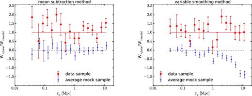
Ratio of the mean equivalent width in stacked spectra to the best-fitting power-law model prediction, for the real data sample (big red circles), and for the average of six mock samples (blue stars). Error bars are computed with the bootstrap method. This ratio should be consistent with zero for the mock sample in the absence of systematic errors, and with unity for the real data if the power-law model provides a good fit to the data.

A2 Tests of the equivalent width measurement for individually detected systems

We now test that the mean equivalent width measured for absorbing systems that are individually clearly detected above the noise agrees with other well-established methods. For this purpose, we use the Mg ii absorber catalogue of Zhu & Ménard (2013b), which contains 35 752 absorption systems from the SDSS DR7 quasar spectra sample. The integrated equivalent widths we obtain for systems in this catalogue, using our two methods of mean subtraction and variable smoothing, are compared with the equivalent widths provided in the catalogue in Fig. A2. There is a large scatter in the equivalent widths obtained with different methods. This result is not surprising, because the noise can change the determination of the continuum in random ways in different methods. In particular, in the method of the mean subtraction, the equivalent width is obtained by integrating the absorbed fraction over a wide interval around the absorber, according to equation (18), adding noise to the estimate. However, the average of the equivalent width estimator in our mean subtraction method, shown by the black points in Fig. A2 (with an rms dispersion indicated by the error bars), agrees very well with the equivalent width provided by the Zhu & Ménard (2013b) catalogue. The variable smoothing method apparently suffers from a bias causing a 10 to 20 per cent increase of the average of the equivalent width (see the black points in middle panel of Fig. A2), which may be due to a tendency of this method to overestimate the continuum level around detected absorption lines.

Figure A2.

Open in new tab Download slide

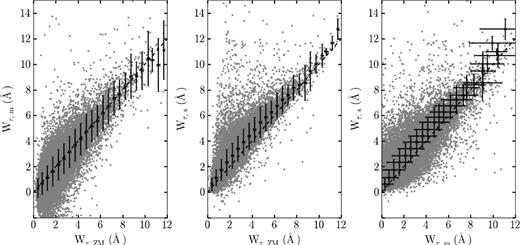
Comparison of the equivalent width estimates from different methods (see Section 3). From left to right, equivalent widths measured using the mean subtraction method, W_m, versus the value of the Zhu and Menard catalogue, W_ZM; variable smoothing method value, W_s, versus W_ZM; and W_s versus W_m. The black points are the average values in bins of ΔW = 0.5 Åin the horizontal axis, with the dispersion in each bin indicated by the error bars. One-to-one correspondence is marked by the black dashed line for visual guidance.

A3 Impact of individually undetected systems on the mean equivalent width

We now test how the presence of weak absorption systems that cannot be individually detected in a single spectrum but contribute to the mean equivalent width as a function of impact parameter from a galaxy can bias the estimate of the quasar continuum in the different methods we use. For this purpose, artificial absorbers are introduced in a spectrum, and then we refit the continuum and measure the change in the measured equivalent width.

As an illustrative example, we have selected a set of 10 random quasar spectra, and we have introduced absorbers at 10 random redshift values and computed the average values for the recovered width. The absorbers are inserted with a double Gaussian profile in the optical depth, as expected for the Mg ii doublet,

\begin{eqnarray} \tau (v) &=& \frac{W_{0}}{\sqrt{2\pi }\sigma } \left( {2\over 3} \exp [-\left(v-v_{1}\right)^{2}/2\sigma ^{2}]\right.\nonumber \\ && \left. +\, {1\over 3} \exp [-\left(v-v_{2}\right)^{2}/2\sigma ^{2}]\right), \end{eqnarray}

(A1)

where W₀ is the total equivalent width of the doublet and σ is velocity dispersion. The zero velocity is conventionally chosen to be the central position of the Mg ii line for an unsaturated line, so that v₁ = −256.05 km s⁻¹ and v₂ = 513.28 km s⁻¹. In the absence of any inserted absorber, the continuum determined in this spectrum is c(v), the flux is f(v), and the transmitted fraction is F(v) = f(v)/c(v). This results in a certain value of the integrated equivalent width W measured over the interval −2000 km s⁻¹ < v < 2000 km s⁻¹, by integrating F(v) over this range. To insert the absorber, the spectral flux is modified according to

\begin{equation} f^{\prime }(v)=f(v)-c(v)\left(1-\exp \left[-\tau (v)\right]\right). \end{equation}

(A2)

Then, a new continuum c′(v) is determined with the new flux, and a new transmitted fraction F ′(v) = f ′(v)/c′(v) is derived. Finally, the new equivalent width W ′ is determined by integrating F ′ over the same velocity interval.

The change in equivalent width caused by the insertion of an absorber, ΔW = W ′ − W, is plotted in Fig. A3 as a function of the equivalent width W_i of the inserted absorber, obtained by integrating 1 − exp[−τ(v)] over the same velocity interval that is used for determining W and W ′ (W_i is nearly equal to W₀ in equation (A1), except that the integrating interval does not extend to infinity). The different lines correspond to different values of the absorber velocity dispersion, σ. The solid blue lines represent the mean subtraction method, and they coincide precisely with ΔW = W_i for all values of σ. The result, as expected, is that the continuum determined by this method is unaffected by the presence of the absorbers that have narrow widths compared to the chosen integrating interval width of 4000 km s⁻¹. The reason is that, in the mean subtraction method, the continuum c′(v) is determined using only the measured flux outside of this interval.

Figure A3.

Open in new tab Download slide

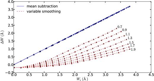
Change in the measured equivalent width, ΔW, caused by the insertion of an absorbing system with equivalent width W_i, for the mean subtraction method (solid blue lines) and the variable smoothing method (dashed red lines). Results are shown as a function of the velocity dispersion σ, with values indicated to the right of the lines in Å. The blue lines all nearly coincide at ΔW = W_i. Points show the values of W_i for which ΔW has been computed; the sudden changes in the red lines indicate discontinuities in the variable smoothing method as the inserted line becomes detected or covers different pixels, which causes a change in the continuum estimate.

On the other hand, the variable smoothing method (dashed red lines in Fig. A3) is strongly biased to lowering the estimated continuum in response to the presence of a weak absorption system. The result is that the change caused by the absorber in the estimated equivalent width, ΔW, can be much less than the true value, and the difference is a complex function of the equivalent width W₀, the velocity dispersion and the S/N of the spectrum. The underestimate of the continuum level is naturally smaller for narrower lines (lower σ), because the lines are detected and eliminated from the continuum estimation for lower values of W₀.

To summarize, the three tests of our continuum fitting methods presented in this appendix demonstrate that the variable smoothing method suffers from several systematic errors. The first test shows that a small negative absorption, of equivalent width ∼− 0.3 km s⁻¹, is induced where there is none. The second test indicates that the equivalent width of strong, detected systems is overestimated by 10–20 per cent. Finally, the third test shows that for weak systems, the continuum is systematically underestimated, thereby strongly reducing the contribution of these systems to the measured equivalent width. However, the mean subtraction method successfully passes all these tests and should therefore provide a reliable estimate of the stacked equivalent width as a function of impact parameter.

Download all slides

Month:	Total Views:
January 2017	1
February 2017	3
March 2017	1
April 2017	1
June 2017	3
August 2017	2
September 2017	1
October 2017	3
November 2017	5
February 2018	4
March 2018	12
April 2018	15
May 2018	10
June 2018	9
July 2018	14
August 2018	6
September 2018	3
October 2018	9
November 2018	10
December 2018	12
January 2019	14
February 2019	14
March 2019	12
April 2019	12
May 2019	17
June 2019	9
July 2019	14
August 2019	12
September 2019	3
October 2019	21
November 2019	12
December 2019	12
January 2020	6
February 2020	14
March 2020	9
April 2020	6
May 2020	5
June 2020	10
July 2020	6
August 2020	7
September 2020	8
October 2020	7
November 2020	5
December 2020	5
January 2021	8
February 2021	4
March 2021	16
April 2021	18
May 2021	14
June 2021	15
July 2021	6
August 2021	9
September 2021	20
October 2021	12
November 2021	16
December 2021	13
January 2022	11
February 2022	24
March 2022	16
April 2022	22
May 2022	18
June 2022	13
July 2022	14
August 2022	19
September 2022	17
October 2022	34
November 2022	12
December 2022	23
January 2023	16
February 2023	17
March 2023	14
April 2023	21
May 2023	22
June 2023	11
July 2023	20
August 2023	13
September 2023	17
October 2023	14
November 2023	15
December 2023	15
January 2024	30
February 2024	21
March 2024	13
April 2024	19

Article Contents

The cross-correlation of Mg ii absorption and galaxies in BOSS

Abstract

1 INTRODUCTION

2 DATA SAMPLE

3 STACKING PROCEDURE

3.1 Method 1: mean subtraction

3.1.1 Generating the mean spectrum

3.1.2 Generating the composite Mg ii absorption spectra

3.2 Method 2: variable smoothing

3.3 Unbiasing the composite spectra

3.4 Bootstrap errors

4 MODEL FOR THE ABSORPTION PROFILE

5 RESULTS

6 DISCUSSION

6.1 Relation of the mean equivalent width to the bias factor of Mg ii absorption systems

6.2 Mean absorption from Mg ii systems

6.3 Derivation of the bias factor of Mg ii systems

6.4 The ratio of Mg ii-absorbing gas to the total mass

7 SUMMARY AND CONCLUSIONS

REFERENCES

APPENDIX A: TESTS OF THE CONTINUUM FITTING METHODS

A1 Systematic errors in the absence of correlations

A2 Tests of the equivalent width measurement for individually detected systems

A3 Impact of individually undetected systems on the mean equivalent width

Citations

Views

Altmetric

Email alerts

Astrophysics Data System

Citing articles via

Latest

Most Read

Most Cited

Article Contents

The cross-correlation of Mg ii absorption and galaxies in BOSS

Abstract

1 INTRODUCTION

2 DATA SAMPLE

3 STACKING PROCEDURE

3.1 Method 1: mean subtraction

3.1.1 Generating the mean spectrum

3.1.2 Generating the composite Mg ii absorption spectra

3.2 Method 2: variable smoothing

3.3 Unbiasing the composite spectra

3.4 Bootstrap errors

4 MODEL FOR THE ABSORPTION PROFILE

5 RESULTS

6 DISCUSSION

6.1 Relation of the mean equivalent width to the bias factor of Mg ii absorption systems

6.2 Mean absorption from Mg ii systems

6.3 Derivation of the bias factor of Mg ii systems

6.4 The ratio of Mg ii-absorbing gas to the total mass

7 SUMMARY AND CONCLUSIONS

REFERENCES

APPENDIX A: TESTS OF THE CONTINUUM FITTING METHODS

A1 Systematic errors in the absence of correlations

A2 Tests of the equivalent width measurement for individually detected systems

A3 Impact of individually undetected systems on the mean equivalent width

Citations

Views

Altmetric

Email alerts

Astrophysics Data System

Citing articles via

Latest

Most Read

Most Cited

This Feature Is Available To Subscribers Only